Machine Learning-Based Investigation of the 3D Printer Cooling Effect on Print Quality in Fused Filament Fabrication: A Cybersecurity Perspective

Abstract

Additive manufacturing (AM), also known as three-dimensional (3D) printing, is the process of building a solid object in a layer-wise manner. Cybersecurity is a prevalent issue that appears more and more frequently as AM becomes popular. This paper focuses on the effect of fan speed on the printing quality and presents a plugin called Fan Speed Attack Detection (FSAD) that predicts and monitors fan speeds throughout the printing process. The goal of the plugin is to prevent cybersecurity attacks, specifically targeting fan speed. Using the proposed FSAD, any fan speed changes during the printing process are evaluated to see whether the printer can sustain the abnormal fan speed change and still maintain good print quality.

1. Introduction

Additive Manufacturing (AM) offers advantages of lightweight production, minimum material waste, and low cost using small working spaces. Different materials, such as metals, polymers, and composites, are used to manufacture parts [1,2]. AM includes four main phases: solid modeling, slicing, 3D printing, and post-processing (such as heat treatment, sintering, etc.). External attacks can happen during any of these phases and the attacks can be classified as sabotage of the printed parts and theft of intellectual property. Due to its young age, there is limited research on the cybersecurity aspect of the AM [3]. In this research, the focus is on the attacks happening during the 3D printing process.

Muhammad et al. considered the four sabotage attacks on the 3D printing process: preventing the filament extrusion to create voids in the printing process, turning on/off and modifying the filament motor to change the density of the printed part, and lastly, changing the nozzle temperature to alter the material properties. The attacks were constrained under the criteria of not being detected; in other words, there must not be any significant changes in the sample geometry after the attacks. After passing the stealthiness test, they performed flexural and bending tests to compare the attacked and no-attack samples for identification [4]. In another study, Gao et al. focused on the changes in infill pattern, nozzle speed, layer height, and fan speed due to attacks. The authors used the accelerometer, magnetometer, and camera to collect data during attacks and proposed an online process monitoring approach to defend the 3D printing process against the attacks [5]. Abdullah et al. proposed an authentication framework to prevent the changes in the part geometry due to attacks on the infill pattern. The researchers installed an in situ optical imaging system to be able to compare the current and solid design infill patterns [6]. Zhou et al. collected the vibration signals from the nozzle/bed and modeled them with an echo state network to detect the unwanted deviations that may occur during the printing process. They used PLA material for the study and samples were in a cubic shape. Their study focused on attacks during the solid modeling stage and printing process [7]. Another study carried out by Moore et al. is based on addressing the cyber-attacks on the printing process by monitoring the electric current delivered to the components of the 3D printer. The authors investigated the changes in G-Code (deleting commands, inserting new commands, etc.) and detected them by measuring the power supply to axis and filament extrusion motors [8]. Wu et al. tried to detect the attacks on infill patterns using a machine learning algorithm. The investigators analyzed five infill pattern types as honeycomb, diamond, linear, star, and catfill. The authors applied three different ML algorithms: random forest, k-nearest neighbor (kNN), and anomaly detection, to detect malicious defects. For each ML algorithm, accuracy results have been compared [9].

Some groups of studies focused on the prediction of surface roughness using machine learning algorithms. Khanzadeh et al. used an unsupervised machine learning (ML) approach to assess the geometric deviations of the AM-produced parts. Their clusters, by using a self-organizing map, quantify the direction and magnitude of geometric deviations [10]. In another study by Zhicheng et al., ML algorithms were used to estimate the size of internal voids, which are significant reasons for geometric inaccuracy. According to their results, support vector regression is worse than neural networks in predicting voids [11]. Zhicheng et al. compared neural networks to linear regression to quantify the dimensional changes of material extrusion-made parts. The neural network approach is better at predicting the dimensional accuracy due to very small p-values and square errors [12].

An ensemble learning-based approach is also used to predict the surface roughness in fused filament fabrication. Li et al. varied layer thickness, extruder temperature, and nozzle velocity for validation of the predictive model. Surface roughness values predicted by the ensemble learning algorithm were compared with the experimental results, and in conclusion, the researchers showed that the proposed model was in good agreement [13]. Wu et al. have developed a data-driven real-time monitoring system to predict the surface roughness of the Fused Filament Fabrication (FFF) printed parts. Predictive models were trained by using the random forest algorithm. The comparison between their predictive models and experimental results shows that the applied algorithm can predict surface roughness values with an error of 5.90% [14]. Lao et al. tried to minimize the surface roughness by using machine learning (artificial neural network (ANN) model). The authors used concrete 3D printing with thirteen different nozzle geometries and the ANN model predicted the nozzle shape according to the extrudate shape by improving the surface finish of the printed parts [15]. Garcia et al. studied the surface finish of the short carbon fiber-reinforced polyethylene terephthalate glycol (PETG) parts by varying the short carbon fiber weight, layer height, surface build angle, number of walls, and printing speed. The researchers determined the significant parameters for the surface roughness and used ML algorithms of random forest and J48 to predict the average surface roughness of the printed part. The authors showed that J48 correctly predicts the surface roughness of the printed part [16]. Another research group investigated the surface roughness of the parts made from polyvinyl butyral using fused filament fabrication. The group selected layer height, nozzle speed, number of perimeters, nozzle temperature, and wall angle as input variables and 48 parts were 3D-printed. The investigators used a total of ten classification algorithms: IBk, BayesNet, NaiveBayes, J48, kStar, random forest, LMT, logistic, SMO, and multilayer perception. According to their results, base algorithm-type functions (SMO/VSM and MLP/NN) predicted the surface roughness better than the others [17]. Liu et al. used a nonparametric Bayesian framework to optimize the quality of the parts manufactured by newly developed 3D printing material. They used Gaussian process regression to predict the surface roughness of the acrylonitrile butadiene styrene polymer with 5% weight graphene. As a result, using the Bayesian framework, the process parameters were optimized after five iterations [18]. Another study by Kandananond predicts the surface roughness of the 3D-printed parts made of polylactic acid (PLA) by comparing two different ML algorithms: Box-Behnken and ANN. Substrate temperature, nozzle speed, and layer height are the input variables and each varied in 3 levels, totaling 80 runs. ANN predicts much better than Box-Behnken according to the results [19]. Tripathi et al. used deep learning to find the relation between 3D printing parameters and surface roughness. The investigators used 11 different input parameters, including layer height, fan speed, nozzle speed, bed temperature, material, etc. Using deep learning, the surface roughness of the final product can be approximated according to their conclusion [20]. In another study by Liu et al., the print quality in additive manufacturing using a physics-informed porosity prediction model was estimated with a 10% to 26% error range [21]. Li et al. introduced a new feature (mean curvature measure) coupled with the training dataset of ML algorithms to detect the defects in 3D-printed parts. For this task, the authors compared five different ML algorithms: linear SVM, gradient boosting, bagging of trees, kNN, and random forest. As in other studies outlined above, random forest yielded the best predictions [22]. A number of researchers proposed acoustic emission and machine learning algorithms to ensure the in situ good print quality. They utilized ANN and support vector machine to predict the surface print quality of the parts [23,24].

Process parameters may be maliciously altered by external attacks, and the largest impact will be on the quality and dimensional accuracy of the printed part. However, an extensive review of the existing literature shows that previous studies considered the stealthiness of the attacks, attacks on the infill pattern, variations in noise generated by the FFF, changes in electric and magnetic properties inside the printer and its components, and prediction of surface roughness by using ML. To the authors’ best knowledge, no research has focused on the relation of the attacks to the printing fan speed and the surface roughness. Our research proves that the variation in fan speed can lead to the detriment of 3D printing output, and hence attacks on it must be prevented. In addition, the research shows that the infill density, layer height, and fan speed have an influence on the surface quality statistically, with a p-value less than 0.05, allowing us to consider these parameters as independent inputs. Finally, an ML algorithm is developed to consider any external disturbances changing the fan speed as cyber-security attacks, and to manage them.

2. Materials and Methods

This section describes the methods that were used in the research process. This includes gathering data, determining the fan speed effect, and creating software. Furthermore, the methods are detailed with the materials used to achieve this progress.

2.1. Determining Fan Speed Effect on the Printing Quality

Surface roughness (SR) is used as a tool to gauge the printing quality. For the subsequent sections, a low SR represents a relatively good printing quality, whereas a high SR represents a poor printing quality.

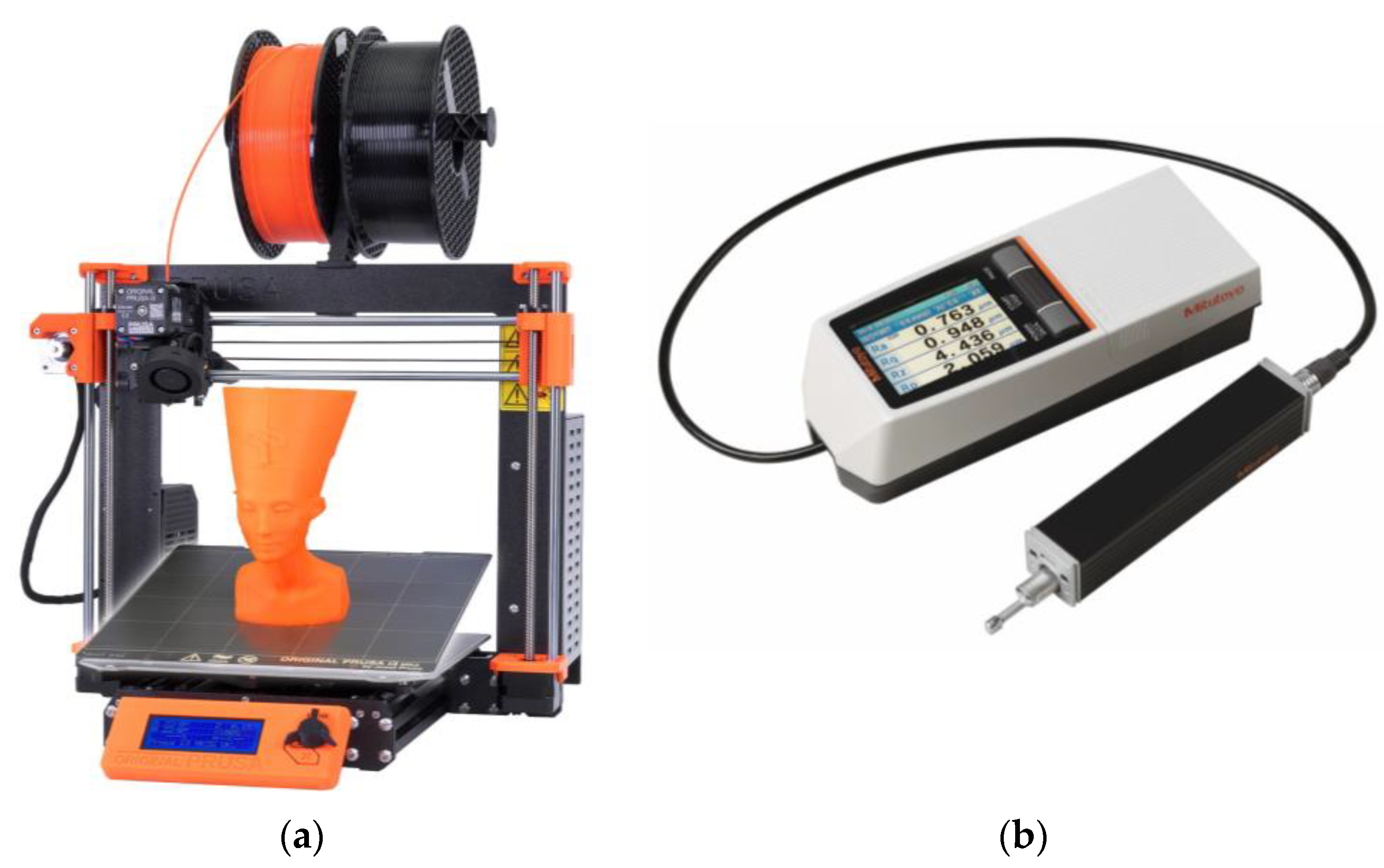
The 3D printer used in this research was a Prusa i3 MK3 printer (Figure 1a), which is made by Prusa Research in Prague, Czech Republic [25]. This printer was selected because it could accurately and quickly manufacture parts. PLA is the most widely used material and it is biodegradable, cheap, and easy to manufacture. Therefore, in this study, PLA manufactured by Push Plastic (Springale, AR, USA) was used for producing the samples. The diameter of the filament was 1.75 mm, the nozzle temperature was 215 °C, and the bed temperature was 50 °C.

To measure the surface roughness of the samples, an SJ-210 surface roughness (SR) tester (Mitutoyo corporation, Aurora, IL, USA) was used. The machine (Figure 1b) permits different surface roughness measuring methods, such as Ra, Rms, Rz, etc., and due to its accuracy and simplicity, Ra was used here. Ra is the arithmetical mean deviation of the measured profile, and its calculation can be shown as:

$$R_a=1/l_m{\int }_0^{l_m}z\left(x\right)dx$$

where $l_m$ is the measured length.

2.2. Data Gathered

There were three parameters used in this research to gather the data, which were:

• Layer thickness (LT): the height of each layer during the printing process.
• Fan speed (FS): the speed of the fan during the FFF process.
• Infill density (ID): the amount of plastic used on the inside of the print.

Layer thickness and infill density were chosen as additional parameters with a hypothesis that they significantly affect the printing process. The validity of the hypothesis was tested using analysis of variance (ANOVA), summarized in the Statistical Analysis Section. Moreover, by measuring these additional parameters, the fan speed’s effect can be measured across a variety of printed objects.

Table 1. Parameters of the study.

LT (mm)	ID (%)	FS (%)
0.1	20	0
0.2	50	25
0.3	80	50
		75
		100

shows the various printing parameters used to evaluate the printing quality effect. According to the table, two parameters were fixed, while the third parameter was varied, for example, fan speeds were changed from 0 to 100% in 25% increments by keeping LT and ID constant.

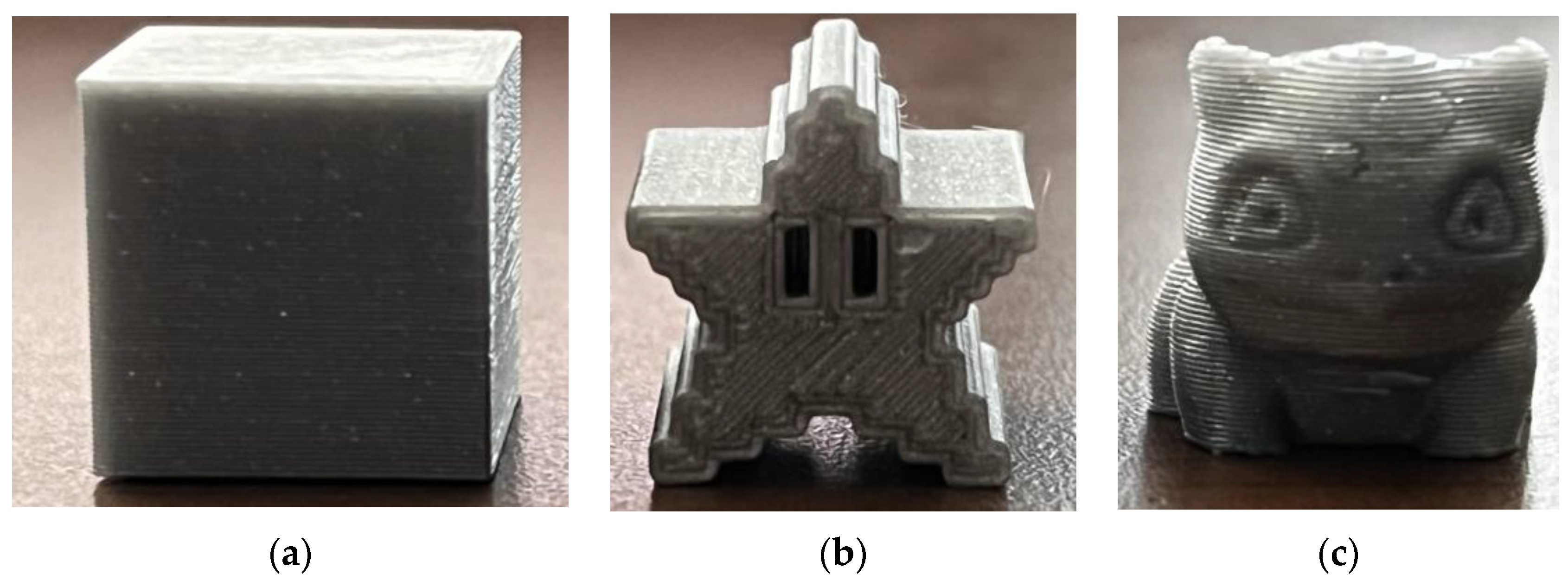
Objects of different types were printed as shown in Figure 2, and they were classified as simple, medium, and complex. The simple object considered in this work was a cubic shape, the medium object was a star, and the complex object was an animal. All solid models were downloaded from the Thingiverse website [27].

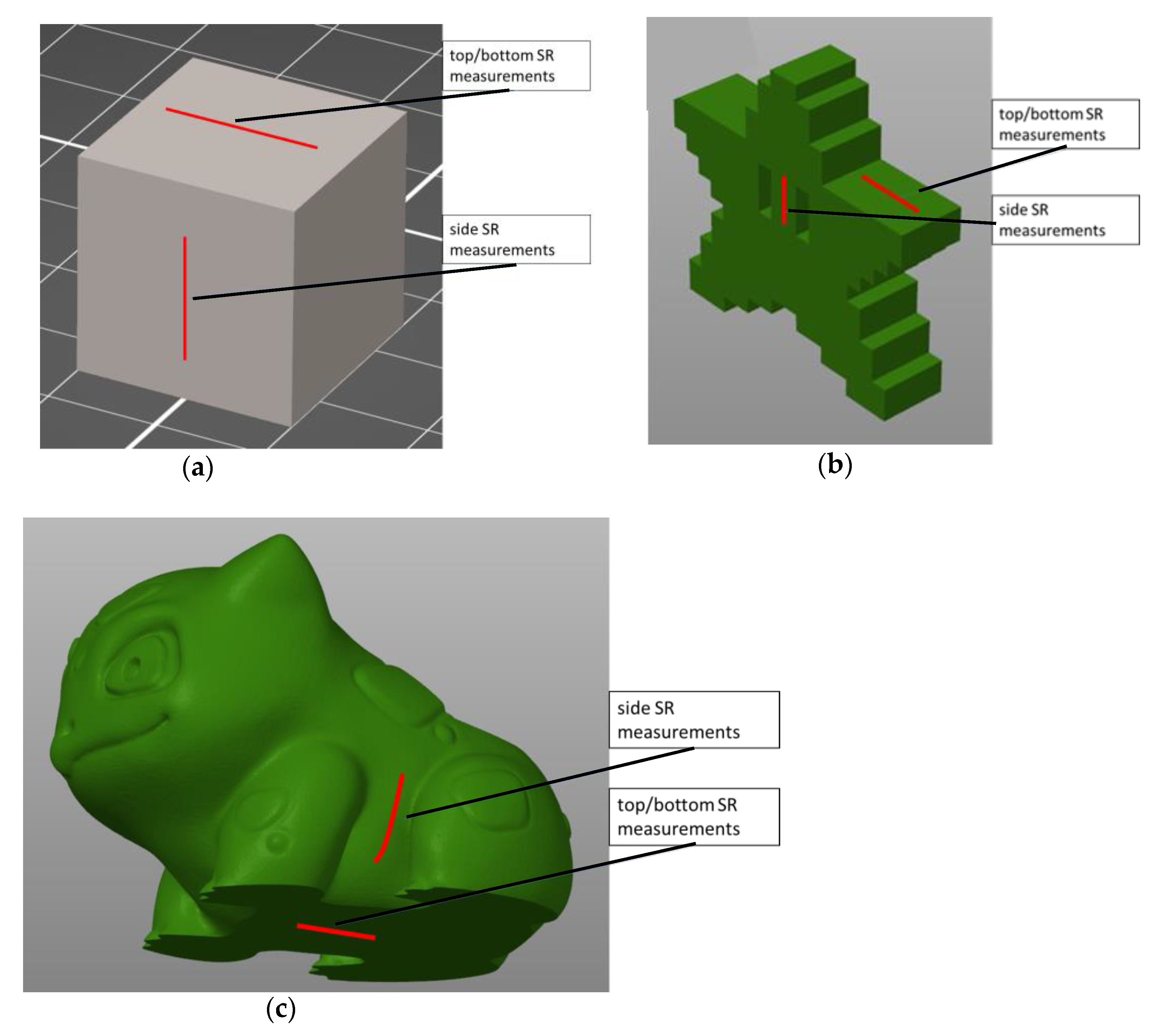
In total, there were 135 combinations of the parameters printed (3 LT × 3 ID × 5 FS × 3 objects = 135 parameters). Then, the SR of each printed object was measured. The faces of the objects were grouped as either top/bottom and side, as shown in Figure 3. For each shape, the top and bottom faces were measured together and so were the sides. Overall, 270 measurements were performed.

K-Means Classification

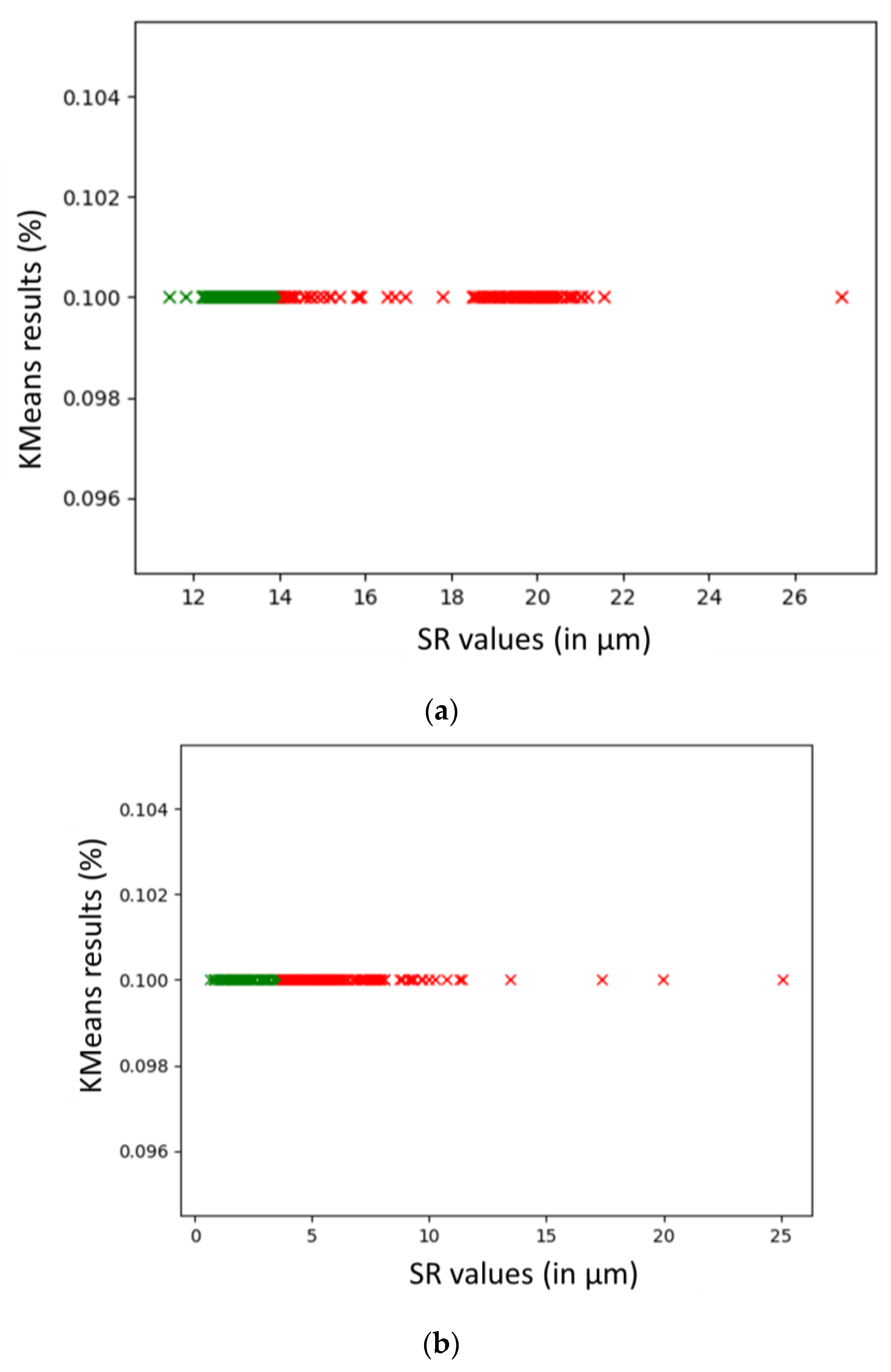
A significant amount of research was carried out using ML, which includes algorithms of K-means clustering, linear regression (LR), and neural network (NN). For K-means, four clusters were used for the dataset collected in Table 1. The K-means algorithm was run using the sci-kit learn package [28], which classifies and splits the data into four cluster groups based on SR, as shown below in Figure 4. From Figure 4a,b, the cluster group that contained the best printing settings for producing the highest printing quality was colored green and called the “optimal group”. The red-colored group in Figure 4a,b represents printing parameters which produced a slightly worse SR than the optimal group. Therefore, these groups were not used.

From the results shown in Figure 4, the best cluster was further analyzed for the fan speed percentages. The percentage of each fan speed was calculated by taking the amount of that particular fan speed in the optimal group and dividing it over the total number of objects in the cluster. As shown in

Table 2. Optimal fan speed percentages for the set best printing quality.

Fan Speed (%)	Side Results (%)	Top/Bottom Results (%)
0	20.00	33.80
25	20.00	16.90
50	20.00	14.08
75	21.08	15.49
100	18.92	19.72

, the side results were relatively ambiguous, being around 20% for each fan speed. The top/bottom results showed that a 0% fan speed was most preferable. The main conclusion for this section is that the fan speed has an effect on the printing quality, with 0% being preferred in most cases. Additionally, the highest SR within this cluster was used further in subsequent analysis as a general threshold, defined as threshSR.

2.3. Fan Speed Attack Detection Plugin

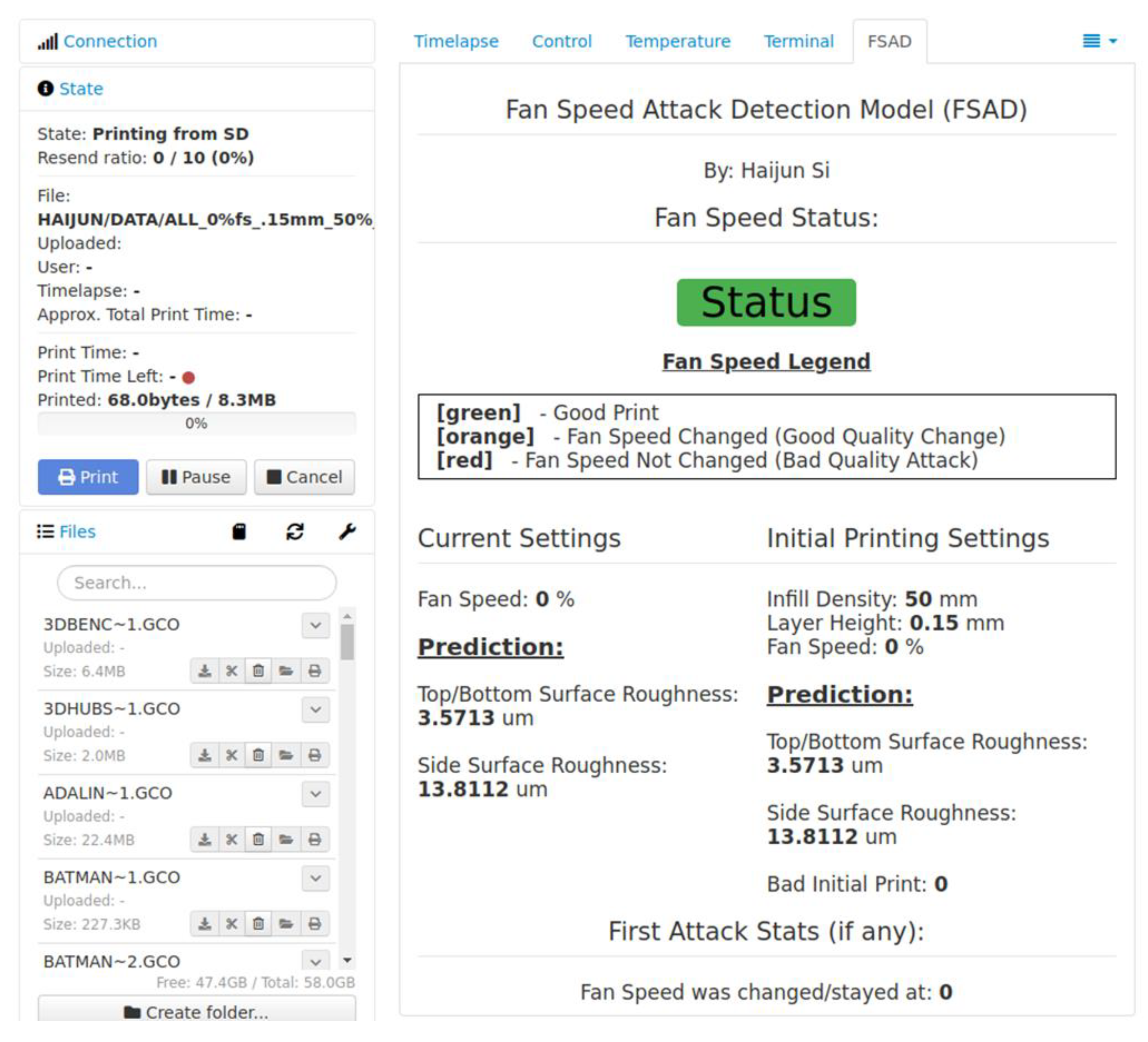
The Fan Speed Attack Detection (FSAD) plugin monitors any incoming fan speed changes during the printing process and uses the G-Code file to predict printing quality. FSAD’s primary purpose is to classify the new fan speed and determine whether to allow the fan speed to change. This plugin has three main components: monitoring fan speed changes, predicting the quality of fan speed changes, and evaluating the printing quality.

2.4. Monitoring Fan Speed Changes

FSAD was developed on a Raspberry Pi and run through a software called OctoPrint [29]. OctoPrint is a web interface that can be remotely run on a Raspberry Pi for monitoring 3D printers. OctoPrint’s developer tools for monitoring the printer status were used to detect when a print starts or ends. This enabled FSAD to start reading the initial printing parameters of LT, ID, and FS. The initial parameters were used to create an initial prediction of the printing quality for comparison to any future fan speed changes. This prediction model is discussed more in detail in the next section, but it was built using NN and predicts a SR considering three parameters.

The intended mechanism created in this research is aimed as a defense against harmful fan speed changes to an ongoing print. The attacker is assumed to be someone with malicious intent in manipulating the fan speed settings and causing harm to the printed product. Furthermore, the attacker is presumed to have capabilities of remotely accessing the printer and interfering with the control settings. Eventually, the proposed ML solution allows for an automated monitoring system that will notify the person(s) if there were an incoming attack. Any incoming fan speed changes are monitored using a G-Code Queued Hook. The G-Code Queued Hook is utilized to read any G-Code commands sent to the printer, specifically targeting fan speed changes. With any incoming fan speed change, a new prediction is generated and compared to the initial prediction and a threshold, which is discussed in Section 2.6. Finally, with any print finishing or canceled state, this plugin is reset to prevent any memory loss or error.

2.5. Prediction Models

The second part of ML used in this research was used for creating a prediction model that can accurately predict surface roughness considering the three parameters: LT, ID, and FS. Linear regression (LR) was created using sci-kit learn [28] and the NN model was created using TensorFlow [30]. The sci-kit learn version 1.2.0 was used and is licensed under the new BSD license. The TensorFlow version is 2.0 and is licensed under the Apache License. LR was used for its simplicity in identifying associations between the three parameters in predicting printing quality. NN was used for its benefits of complexity and flexibility with hidden layers [12]. The metric used to measure the accuracy of each model was mean absolute error (MAE), which is the difference between the predicted and actual SR. The performance of each model was measured this way because the models provide a solution to a regression problem, one in which the lowest MAE would result in the best SR. Both models used the top/bottom and side datasets for training and testing data, which were run with K-fold cross-validation. K-fold cross-validation is a re-sampling procedure used to test the validity and measure the accuracy of the data. The data were run with 5-fold cross-validation, meaning that 80% of the data was used for training and 20% was used for testing. This method was then repeated 5 times, where each 20%of the data was tested against the other 80% of the data, ensuring a consistent MAE.

2.5.1. Linear Regression

The model used K-fold cross-validation to produce accurate results across all the data. The predicted results from each K-fold were measured for MAE and averaged over the total number of folds. These MAE results for both measurements are depicted below in

Table 3. Linear regression.

Model	MAE
Side	1.385
Top/bottom	1.860

.

2.5.2. Neural Networks

The NN model was outlined with an input layer with 3 parameters, 6 hidden layers with 128 neurons each, and 1 output layer, which was the predicted SR. The activation function used was ReLU and the optimizer was Adam. NN resulted in far better accuracy, as shown in

Table 4. Neural networks.

Model	MAE
Side	0.4661
Top/bottom	1.696

. Therefore, the NN model was deployed and used in the plugin development through TensorFlow lite. TensorFlow lite is a library used for deploying ML models on mobile devices.

2.6. Classification for Print Quality

The conditions for any new fan speed change were decided based on two tolerance thresholds, low and high tolerance. The selection of the tolerance was determined based on the initial prediction of the original parameters. Once selected from the initial prediction, this tolerance would be used to compare to newly predicted SR with any fan speed changes.

If the initial SR prediction was worse than threshSR, then the tolerance would be set to low. Low tolerance compares any newly predicted SR to the sum of the initial predicted SR and the measured error, which is the NN MAE. This essentially imposes the policy that the new SR prediction must be lower than the initial prediction. Vice versa, with the initial prediction being better than the threshSR, the tolerance would be set to high. High tolerance compares any newly predicted SR to the sum of threshSR and NN MAE. This ensures that the new fan speed remains within an optimal printing quality range.

There are two different tolerances for fan changes, which are:

Low tolerance (LT) = initial predicted SR + NN MAE

High tolerance (HT) = threshSR + NN MAE

Two algorithms were developed in the research and named as Algorithm 1 and Algorithm 2. Algorithm 1 classifies the initial printing parameters with a prediction that will be the condition for fan changes during the printing process. Based on the initial prediction compared with high tolerance, this algorithm returns either LT or HT. Algorithm 2 classifies new fan speed changes by comparing the new prediction with the tolerance. If the new prediction is greater than the tolerance, the new fan speed is not to be used, otherwise the new fan speed is allowed to be sent to the printer.

2.7. Statistical Analysis

Two main assumptions to perform an analysis of variance (ANOVA) are the normality test and equal variances. Residual normality of both the side and top/bottom surface roughness values was checked by using the Anderson–Darling test, and Levine’s test was used for the equal variance assumption. The calculations were performed in Minitab statistical software version 21.3.1, and in both cases, the p-value was greater than a significance level of 5%, hence allowing us to use the linear model for the statistical analysis. The p-values were calculated for each factor, as shown in

Table 5. ANOVA results.

Source	Location	DF	p-Value
Infill density	SR_side	2	0.333
Layer thickness	SR_side	2	$<{10}^{-5}$
Fan speed	SR_side	4	0.026
LT × ID	SR_side	4	0.746
ID × FS	SR_side	8	0.651
LT × FS	SR_side	7	0.063
LT × ID × FS	SR_side	13	0.606
Infill density	SR_top/bottom	2	0.430
Layer thickness	SR_top/bottom	2	$<{10}^{-12}$
Fan speed	SR_top/bottom	4	0.020
LT × ID	SR_top/bottom	4	0.207
ID × FS	SR_top/bottom	8	0.666
LT × FS	SR_top/bottom	7	0.346
LT × ID × FS	SR_top/bottom	13	0.267

, and they were calculated separately for top/bottom and side surfaces, as shown under the column of location. According to the analysis results, the infill density did not have statistical influence on the variation of the surface roughness, where in both cases the value was greater than 0.05. Layer height had the highest influence, with an almost 0 p-value, followed by fan speed with 0.026 for side and 0.020 for top/bottom surfaces. The p-values of interactions between the factors were also calculated, with the lowest value for the layer thickness and fan speed interaction; however, the value was greater than the level of significance, and hence, there was no statistical influence on the dependent variable.

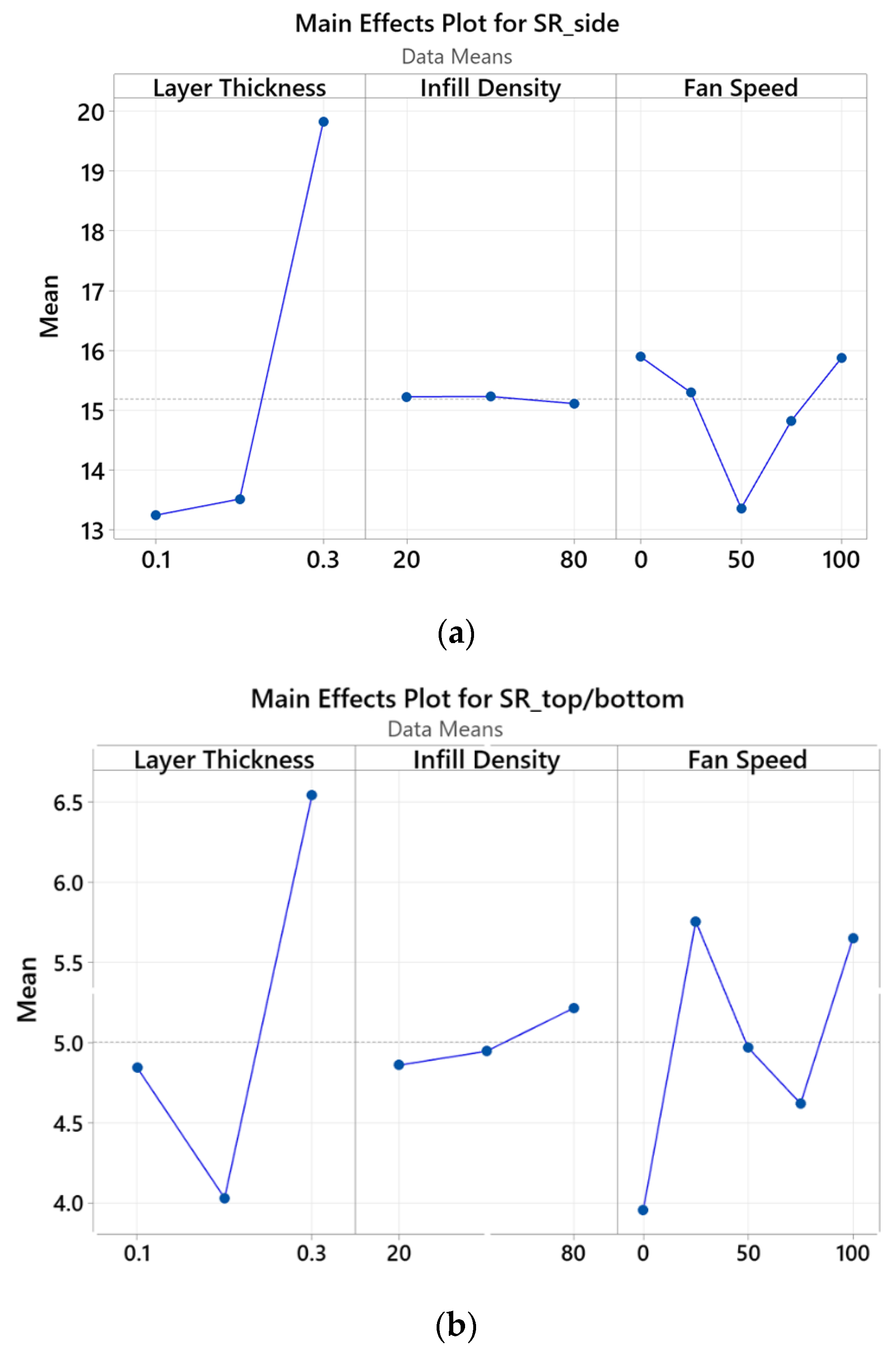
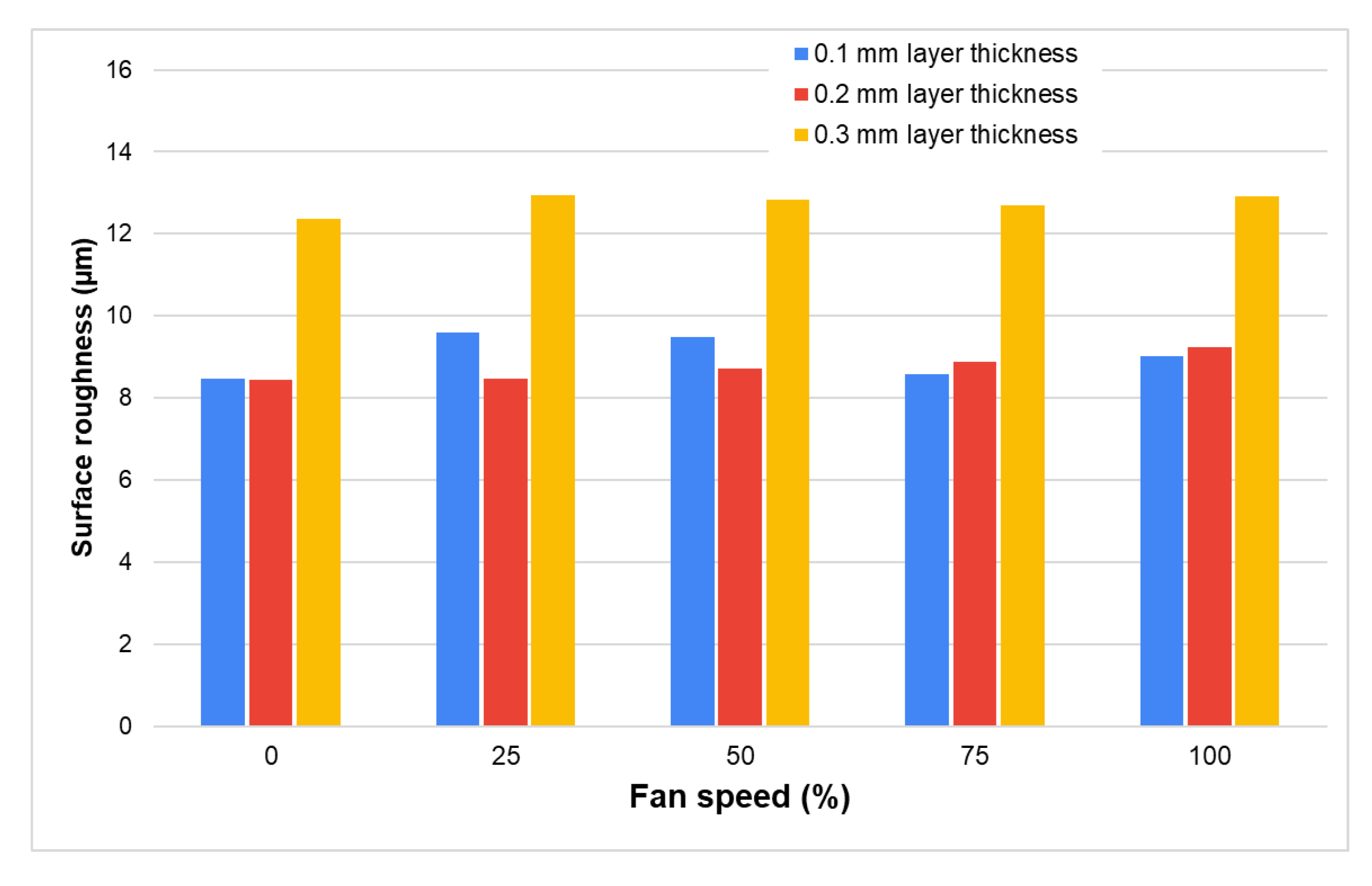
The main effects are shown in Figure 5. As illustrated in the figure, the layer thickness was the most influential factor in both the side and top/bottom SR measurements, with a non-linear variation. The impact was more significant with a layer thickness change of 0.2 to 0.3 mm, which is acceptable since higher layer thickness values decrease the resolution of the part, hence resulting in less dimensional accuracy. The infill density effect was very minimal, and it was almost a constant horizontal line concentrated about the mean values of 15 and 5 for the side and the top/bottom SR, respectively. In addition, the fan speed effect also had an impact on the SR results, again in a non-linear fashion, but the impact was not as pronounced in the case of layer thickness. Since the SR values were calculated at different layer heights, the overall impact cannot be seen in this chart; thus, a separate calculation was performed for finding the average SR values while fixing the layer height at 0.1, 0.2, and 0.3 mm values. According to the results, minimum surface roughness occurred at a 0% fan speed value, with average SR values of 8.472 µm at 0.1 mm LT, 8.430 µm at 0.2 mm LT, and 12.369 µm at 0.3 mm LT.

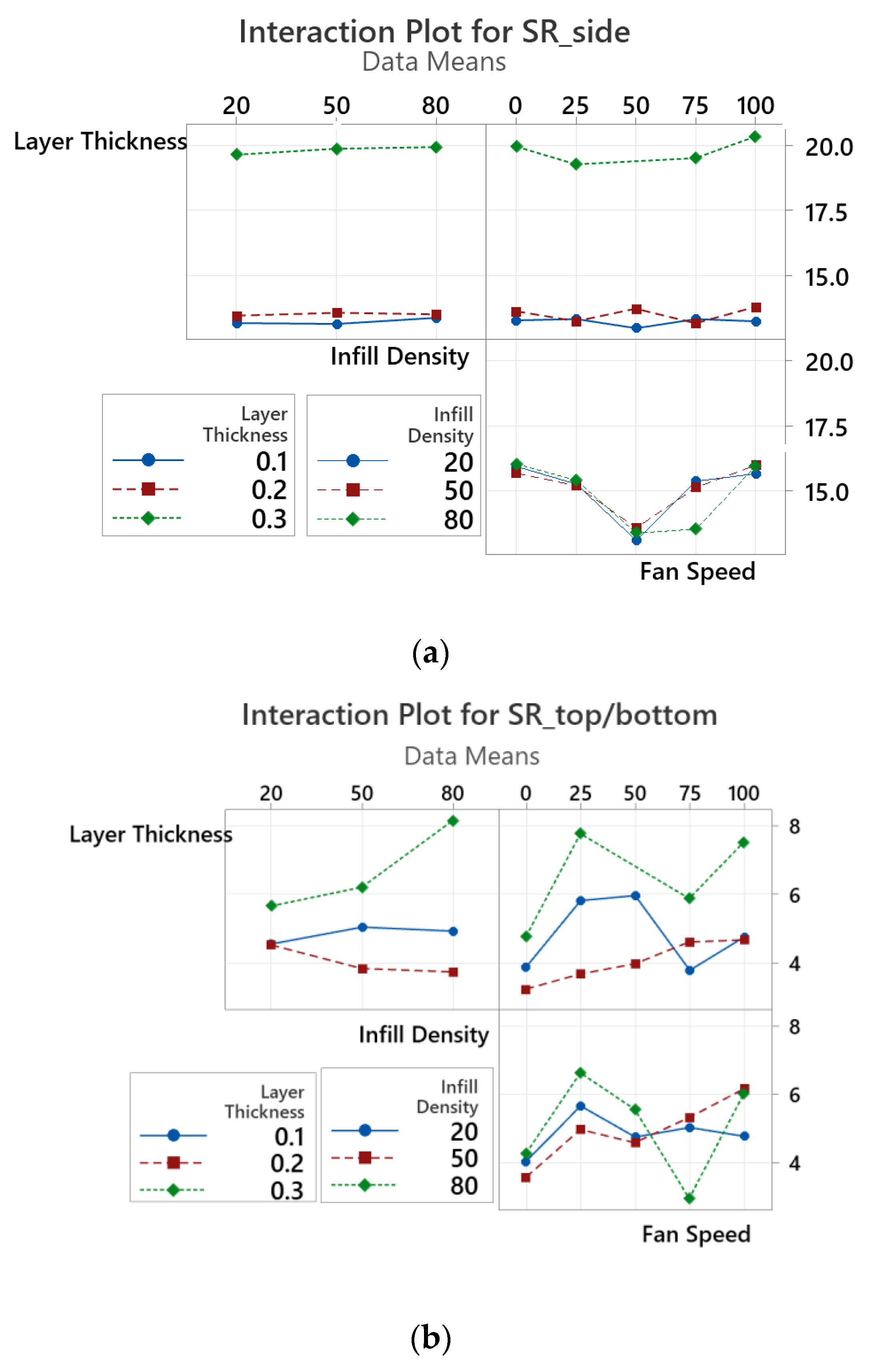
Finally, interaction plots between LT, ID, and FS are illustrated in Figure 6 using ANOVA in Minitab. The layer thickness and infill density interaction were ordinal in both side and top/bottom SR experiment results. It can be seen from the interaction plot between layer thickness and infill density that SR was maximum at a 0.3 mm layer height, independent of the infill density for side SR, however for the top/bottom surfaces, the maximum value of the SR was sensitive to the variation of ID, and it increased linearly as ID increased from 50% to 80%. The interaction between LT and FS affected SR again at higher LT values, and the minimum SR occurred at a 0% FS, as discussed before. On the contrary, the LT and FS interaction plot for top/bottom SR was more erratic, with SR achieving its minimum value at a 0% FS again in all LT variations. Moreover, the ID and FS plot inside SR obtained almost the same values at all ID in each FS, again proving the higher p-value of the ID. The non-ordinal interaction plot of ID and FS in the top/bottom measurements had a possible outlier at 75%, which is also discussed in the next section, and excluding the outlier, ID did not statistically affect the results of SR measurements and the best print quality occurred with the lowest value of FS and a medium ID of 50%.

According to the ANOVA residual plot versus the fitted value, some experimental values were possible outliers. To test those points, Grubb’s test was used, which showed 7 suspected extreme values as outliers for 100% FS, 0.3 mm LH, and 1 for 25% FS, 0.3 mm LH. One more validation study was performed, and here, the average print quality was calculated with and without the outliers at each fan speed, fixing the layer thickness. According to the results of the calculations, including the outliers caused inconsistent behavior in the print quality at a 25% FS for side measurements and 100% for top/bottom measurements, which is not possible in the real 3D printing process. The reason for the outliers may be the measurement tool error, because at higher layer height values, SR sharply increased, affecting the sensitivity of the machine. Therefore, those points were removed, and the average print quality was calculated as illustrated in Figure 7. According to the figure, the best print quality was achieved at a 0% FS, with values increasing with higher fan speeds, except with slight fluctuations at a 75% and 100% FS for 0.1 mm LH. The variation at those points was in the order of less than 0.5 µm and it can depend on random errors due to changes in ambient humidity and temperature values, operator errors, etc., which can be neglected.

3. FSAD Results and Discussion

Figure 8 shows the user interface for FSAD. The main component of the interface is the status button, which has three settings: green, orange, and red. The green status signifies that there has been no attempted fan speed change during the printing process. The orange status represents a warning to the user that there has been an attempted fan speed change. However, the new fan speed in this status does not affect the printing quality, and therefore it is an allowed change during the printing process and the current settings also match that change.

The red status shows that there has been an attempted fan speed change and the change would result in poor printing quality. Due to this, the fan speed has not changed, and neither have any of the settings. The rest of the interface shows the original printing settings and predictions, along with the latest prediction and the fan speed.

4. Conclusions and Future Work

The purpose of this research was to determine the effect of fan speed on the printing quality. For this purpose, K-means algorithm and linear regression techniques have been used with the advantages of less computation time and resources. In addition, ANOVA has been applied to check the interaction between printing parameters and their statistical influence on the response variable. According to the data collected from various process parameters and the classification of SR groups, the printing quality was significantly affected by the fan speed. Therefore, a plugin has been developed to warn users about external fan speed changes and defend against malicious attacks that would negatively alter the quality of the printed part. As a case study, the plugin was successfully run on a Prusa i3 MK3 printer. Each aspect of the plugin was thoroughly tested. Three different statuses have been identified to show the extremity of the abnormal fan speed changes.

For future work, a more accurate result may be achieved with additional data gathered on a wider range of parameters. The plugin can currently only process PrusaSlicer G-Code, so being able to process any type of G-Code would allow for more abstract functionality. In addition, other different ML algorithms may be used for optimization in terms of inference time, accuracy, and model size.