Unsteady Viscous Incompressible Bingham Fluid Flow through a Parallel Plate

Abstract

Numerical investigation for unsteady, viscous, incompressible Bingham fluid flow through parallel plates is studied. The upper plate drifts with a constant uniform velocity and the lower plate is stationary. Both plates are studied at different fixed temperatures. To obtain the dimensionless equations, the governing equations for this study have been transformed by usual transformations. The obtained dimensionless equations are solved numerically using the explicit finite difference method (FDM). The studio developer Fortran (SDF) 6.6a and MATLAB R2015a are both used for numerical simulations. The stability criteria have been established and the system is converged for Prandtl number $P_r\ge 0.08$ with $\Delta Y=0.05$ and $\Delta \mathsf{\tau }=0.0001$ as constants. As a key outcome, the steady-state solutions have been occurred for the dimensionless time $\mathsf{\tau }=4.00$ The influence of parameters on the flow phenomena and on shear stress, including Nusselt number, are explained graphically. Finally, qualitative and quantitative comparison are shown.

1. Introduction

A Bingham fluid is a non-Newtonian viscoplastic fluid that possesses a yield strength that must be outstripped before the fluid will flow. In many geological and industry materials, Bingham fluids are used as a general mathematical basis of mud flow in drilling engineering, including in the handling of slurries, granular suspensions, etc. Bingham fluid is named after Eugene C. Bingham, who declared its mathematical explanation.

In this regard, an exploration of the laws for plastic flow has been studied by Bingham [1]. Darby and Melson [2] formulated an empirical expression to guess the friction loss factor for the drift of a Bingham fluid. Bird et al. [3] analyzed the rheology and flow phenomena of viscoplastic materials. Convective heat transfer for Bingham plastic inside a circular pipe and the numerical approach for hydro-dynamically emerging flow and the simultaneously emerging flow were studied by Min et al. [4]. Liu and Mei [5] considered the slow spread of a Bingham fluid sheet on an inclined plane. For Bingham fluids, the Couette–Poiseuille flow between two porous plates, taking slip conditions into consideration, was investigated by Chen and Zhu [6]. Sreekala and Kesavareddy [7] mentioned the Hall impacts on magneto-hydro dynamics (MHD) Bingham plastic flow over a porous medium, including uniform suction and injection. For Bingham fluids, the MHD flow for an unsteady case considering Hall currents was described by Parvin et al. [8]. Rees and Bassom [9] considered Bingham fluids over a porous medium following a rapid modification of surface heat flux.

Mollah et al. [10] numerically studied the ion-slip and Hall impacts for MHD Bingham fluid flowing through parallel plates, including the considerations of unsteady cases and suction. Gupta et al. [11] considered the MHD mixed convective stagnation point flow and the heat transfer of an incompressible nano fluid over an inclined stretching sheet. Mollah et al. [12] investigated Bingham fluid flow through an oscillatory porous plate with an ion-slip and hall current.

Along with these studies, our aim is to numerically investigate unsteady Bingham fluid flow between parallel plates. The current study is concerned with the generalized Ohm’s law considering the ion-slip and Hall current is absent. Additionally, the Couette flow is considered where the viscous dissipation, pressure gradient, and rheology of Bingham fluids are involved. The explicit FDM has been used to demonstrate the dimensionless non-linear, coupled, partial differential equations. The achieved results are shown graphically.

2. Mathematical Formulation

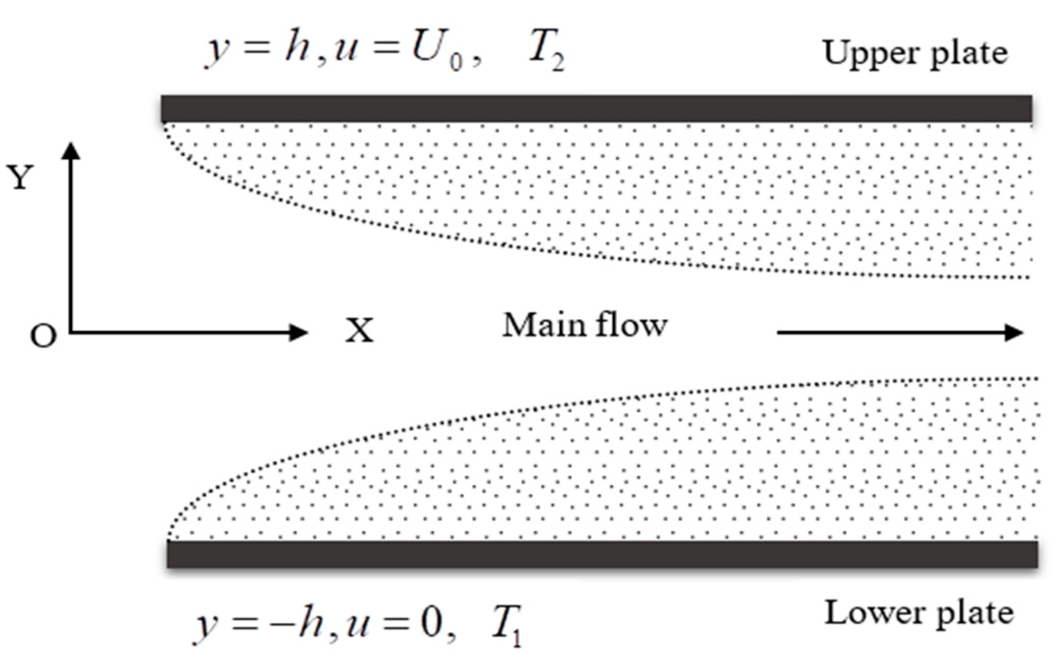
The physical configuration of the considered problem that corresponds with the boundary conditions is shown in Figure 1. A laminar, incompressible, non-Newtonian Bingham fluid is considered to be flowing among two infinite plates situated at the $y=\pm h$ planes and lengthening from $x=0\mathrm{to}\infty$.

The upper plate has a uniform velocity, $U_0$ and the lower plate is stationary. Two constant temperatures, $T_2\mathrm{and}{T}_1$ are considered respectively for both upper and lower plates, where $T_2>T_1$. A constant pressure gradient $\frac{dP}{dx}$ is driven on the fluid along $X$-direction and the body force are neglected.

Within the above considerations, the model is governed by the following equations:

• Continuity equation:

  $$\frac{\partial u}{\partial x}+\frac{\partial v}{\partial y}=0$$

  (1)
• Momentum equation:

  $$\frac{\partial u}{\partial t}+u\frac{\partial u}{\partial x}+v\frac{\partial u}{\partial y}=-\frac{1}{\rho }\frac{dp}{dx}+\frac{1}{\rho }\frac{\partial }{\partial y}\left(\mu \frac{\partial u}{\partial y}\right)$$

  (2)
• Energy equation:

  $$\frac{\partial T}{\partial t}+u\frac{\partial T}{\partial x}+v\frac{\partial T}{\partial y}=\frac{\mathsf{\kappa }}{c_p\rho }\left(\frac{{\partial }^{2}T}{\partial y^2}\right)+\frac{\mu }{\rho c_p}{\left(\frac{\partial u}{\partial y}\right)}^2$$

  (3)

  where the apparent viscosity of the Bingham fluids:

  $$\mu =\mathsf{{\rm K}}+\frac{{\tau }_0}{\frac{\partial u}{\partial y}}$$

  (4)

  where $\mathsf{{\rm K}}$ represents the plastic viscosity of the Bingham fluid and ${\tau }_0$ represents the yield stress.

The corresponding initial and boundary conditions can be given as follows:

$t\le 0,u=0,T=T_1$ everywhere

$$\begin{array}{c}u=0,T=T_{1}atx=0\\ t>0,u=0,T=T_{1}aty=-h\\ u=U_0,T=T_{1}aty=h\end{array}$$

(5)

For the numerical solution, the above Equations (1)–(5) are required to transfer dimensionless form. The dimensionless quantities (6) that have been used which are considered as follows:

$$X=\frac{x}{h},Y=\frac{y}{h},U=\frac{u}{U_0},V=\frac{v}{U_0},\tau =\frac{t{U}_0}{h},\theta =\frac{T-T_1}{T_2-T_1},\overline{\mu }=\frac{\mu }{\mathsf{{\rm K}}},\mathsf{{\rm P}}=\frac{\mathrm{p}}{\rho U_0^2}$$

(6)

The non-dimensional variables (6) are used in Equations (1)–(5) to obtain the dimensionless governing Equations (7)–(11):

$$\frac{\partial U}{\partial X}+\frac{\partial V}{\partial Y}=0$$

(7)

$$\frac{\partial U}{\partial \tau }+U\frac{\partial U}{\partial X}+V\frac{\partial V}{\partial Y}=-\frac{dP}{dX}+\frac{1}{R_e}\frac{\partial }{\partial Y}\left(\overline{\mu }\frac{\partial U}{\partial Y}\right)$$

(8)

$$\frac{\partial \theta }{\partial \tau }+U\frac{\partial \theta }{\partial X}+V\frac{\partial \theta }{\partial Y}=\frac{1}{P_r}\left(\frac{{\partial }^2\theta }{\partial Y^2}\right)+E_c\overline{\mu }{\left(\frac{\partial U}{\partial Y}\right)}^2$$

(9)

where

$$\overline{\mu }=1+\frac{{\tau }_D}{\frac{\partial U}{\partial Y}}$$

(10)

The non-dimensional parameters are as follows:

• Bingham number, ${\tau }_D=\frac{{\tau }_{0}h}{\mathsf{{\rm K}}{U}_0}$; Reynolds number, $R_e=\frac{\rho U_{0}h}{\mathsf{{\rm K}}}$; Prandtl number, $P_r=\frac{\rho c_p{U}_{0}h}{k}$; and
• Eckert number, $E_c=\frac{U_{0}K}{\rho c_{p}h\left(T_2-T_1\right)}$.

The subjected dimensionless conditions can be noted as follows:

$\tau \le 0,U=0,\theta =0$ everywhere

$$\begin{array}{c}U=0,\theta =0atX=0\\ \tau >0,U=0,\theta =0atY=-1\\ U=1,\theta =1atY=1\end{array}$$

(11)

3. Shear Stress and Nusselt Number

The shear stresses at both the stationary and moving plates are studied from the velocity profile. The local shear stress in $X$-direction for stationary plate is ${\tau }_{L1}={\left(\mu \frac{\partial U}{\partial Y}\right)}_{Y=-1}$ and for the moving plate is ${\tau }_{L2}={\left(\mu \frac{\partial U}{\partial Y}\right)}_{Y=1}$. Moreover, the rate of heat transfer, or the Nusselt number, for the stationary and moving plates are studied from the temperature fields. The Nusselt number in the $X$-direction for the stationary plate is $N_{u_{L1}}=\frac{{\left(\frac{\partial T}{\partial Y}\right)}_{Y=-1}}{-T_m}$ and for the moving plate is $N_{u_{L2}}=\frac{{\left(\frac{\partial T}{\partial Y}\right)}_{Y=1}}{-\left(T_m-1\right)}$, where $T_m$ is the dimensionless mean fluid temperature and is given by $T_m=\frac{{{\displaystyle \int }}_{-1}^{1}U\theta dY}{{{\displaystyle \int }}_{-1}^{1}UdY}$.

4. Numerical Technique

A set of finite difference approaches are required to solve dimensionless coupled non-linear partial differential Equations (7)–(10). The dimensionless coupled non-linear partial differential Equations (7)–(10) have been solved by using explicit FDM, subject to the boundary conditions (11). There are number of experiments to solve this kind of unsteady time-dependent problem using FDM where the pressure gradient is constant. The stability and convergence criteria of the explicit FDM are established for finding the restriction of the values of various parameters to get converged solutions (Mollah et al. [10,12] and Akter et al. [13]).

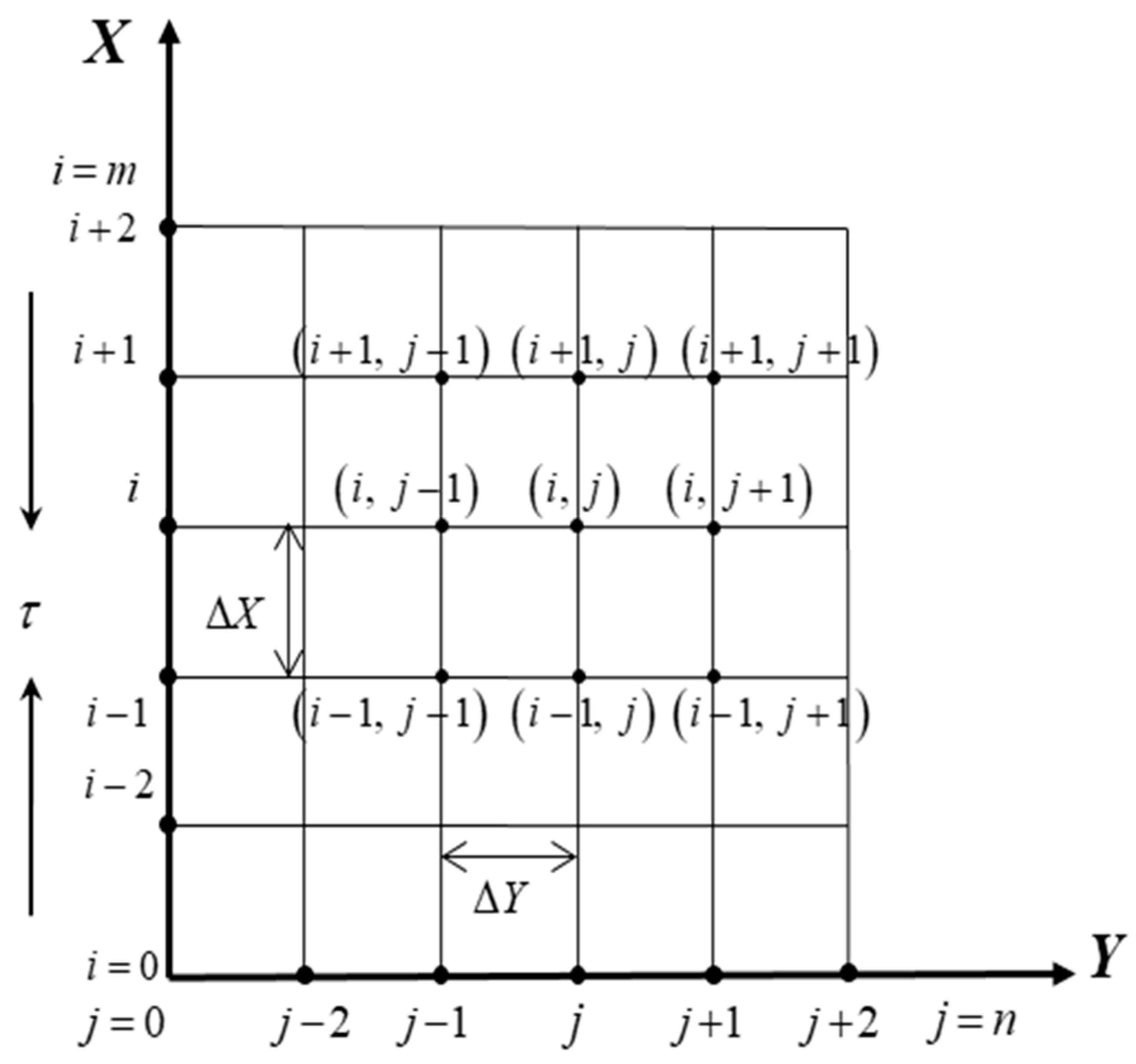
Here, the region inside the boundary layer is distributed into grid spaces of lines parallel to the $X$ and $Y$ axes; where the $X$ axis is towards the plate and $Y$ axis is normal to the $X$ axis. It is determined that the height of the plate is $X_{max}=\left(40\right)$, i.e., $X$ extends from 0 to 40 and $Y_{max}=\left(2\right)$ which corresponds to $Y\to \infty$, i.e., $Y$ limits from 0 to 2 (length). There are $m=40\mathrm{and}n=40$ grid spacing lines in the $X$ and $Y$ directions, respectively, as shown in Figure 2. It is shown that $\Delta X$ and $\Delta Y$ are constant mesh or grid space lines towards $X$ and $Y$ directions, respectively, and is noted as follows, $\Delta X=1.0\left(0\le x\le 40\right)$ and, with the smaller time-step of $\Delta \tau =0.0001$.

$U^{\prime }$ and ${\theta }^{\prime }$ denote the values of $U$ and $\theta$ at the last step of time, respectively. By applying the explicit FDM, the set of finite difference equations for the model are expressed as follows:

$$\frac{U_{i,j}-U_{i-1,j}}{\Delta X}+\frac{V_{i,j}-V_{i,j-1}}{\Delta Y}=0$$

(12)

$$\begin{array}{c}\frac{U_{i,j}^{\prime }-U_{i,j}}{\Delta \tau }+U_{i,j}\frac{U_{i,j}-U_{i-1,j}}{\Delta X}+V_{i,j}\frac{U_{i,j}-U_{i,j-1}}{\Delta Y}=-\frac{dP}{dX}\\ +\frac{1}{R_e}\left[\left(\frac{{\overline{\mu }}_{i,j}-{\overline{\mu }}_{i,j-1}}{\Delta Y}\right)\left(\frac{U_{i,j}-U_{i,j-1}}{\Delta Y}\right)+{\overline{\mu }}_{i,j}\left(\frac{U_{i,j+1}-2U_{i,j}+U_{i,j-1}}{{\left(\Delta Y\right)}^2}\right)\right]\end{array}$$

(13)

$$\begin{array}{c}\frac{{\theta }_{i,j}^{\prime }-{\theta }_{i,j}}{\Delta \tau }+U_{i,j}\frac{{\theta }_{i,j}-{\theta }_{i-1,j}}{\Delta X}+V_{i,j}\frac{{\theta }_{i,j}-{\theta }_{i,j-1}}{\Delta Y}=\frac{1}{P_r}\frac{{\theta }_{i,j+1}-2{\theta }_{i,j}+{\theta }_{i,j-1}}{{\left(\Delta Y\right)}^2}\\ +E_c\left({\overline{\mu }}_{i,j}\right)\left[{\left(\frac{U_{i,j}-U_{i,j-1}}{\Delta Y}\right)}^2\right]\end{array}$$

(14)

$${\overline{\mu }}_{i,j}=1+\frac{{\tau }_D}{\left(\frac{U_{i,j}-U_{i,j-1}}{\Delta Y}\right)}$$

(15)

Further, the finite difference subjected conditions may be described as follows:

$$\begin{array}{c}{U}_{i,L}=0,{\theta }_{i,L}=0atL=-1\\ U_{i,L}=1,{\theta }_{i,L}=1atL=1\end{array}$$

(16)

5. Stability and Convergence Analysis

The stability and convergence criteria of the explicit FDM are established for finding the restriction of the values of various parameters to get converged solutions. Excluding the stability criteria and convergence analysis of the acquired finite difference method, the analysis will remain incomplete unless an explicit process is being used. For the constant grid spaces, the stability analyses of the design have been performed as follows.

Equations (12) and (15) will be disregarded, because $\Delta \tau$ does not exist. At a time arbitrarily called $t=0$, the Fourier expansion for $U$ and $\theta$ at are all $e^{i\alpha X}{e}^{i\beta Y}$ apart from a constant, where $i=\sqrt{-1}$. The expressions for $U$ and $\theta$ at time $t=\tau$ can be defined as follows:

$$\begin{array}{c}U:\psi \left(\tau \right)e^{i\alpha X}{e}^{i\beta Y}\\ \theta :\varphi \left(\tau \right)e^{i\alpha X}{e}^{i\beta Y}\end{array}$$

(17)

After the time-step, these terms have taken the form as follows:

$$\begin{array}{c}U:{\psi }^{\prime }\left(\tau \right)e^{i\alpha X}{e}^{i\beta Y}\\ \theta :{\varphi }^{\prime }\left(\tau \right)e^{i\alpha X}{e}^{i\beta Y}\end{array}$$

(18)

Substituting Equations (15) and (17) into Equations (13) and (14), concerning the coefficients $U$ and $V$ as constants over any one time-step, the obtained equations can be described as follows:

$$\frac{{\psi }^{\prime }\left(\tau \right)-\psi \left(\tau \right)}{\Delta \tau }+U\frac{\psi \left(\tau \right)\left(1-e^{-i\alpha \Delta X}\right)}{\Delta X}+V\frac{\psi \left(\tau \right)\left(1-e^{-i\beta \Delta Y}\right)}{\Delta Y}=0$$

(19)

$$\frac{{\varphi }^{\prime }\left(\tau \right)-\varphi \left(\tau \right)}{\Delta \tau }+U\frac{\varphi \left(\tau \right)\left(1-e^{-i\alpha \Delta X}\right)}{\Delta X}+V\frac{\varphi \left(\tau \right)\left(1-e^{-i\beta \Delta Y}\right)}{\Delta Y}=\frac{1}{P_r}\left[\frac{2\varphi \left(\tau \right)\left(\cos \beta \Delta Y-1\right)}{{\left(\Delta Y\right)}^2}\right]$$

(20)

The simplification of Equations (19) and (20) can be denoted in matrix form, and are expressed as follows:

$$\left[\begin{array}{c}{\psi }^{\prime }\\ {\varphi }^{\prime }\end{array}\right]=\left[\begin{array}{cc}A& 0\\ 0& B\end{array}\right]\left[\begin{array}{c}\psi \\ \varphi \end{array}\right],\mathrm{that}\mathrm{is}{\eta }^{\prime }=T\eta$$

(21)

where,

$$\begin{array}{l}{\eta }^{\prime }=\left[\begin{array}{c}{\psi }^{\prime }\\ {\varphi }^{\prime }\end{array}\right],T=\left[\begin{array}{cc}A& 0\\ 0& B\end{array}\right],\eta =\left[\begin{array}{c}\psi \\ \varphi \end{array}\right],A=1-\frac{U\Delta \tau }{\Delta X}\left(1-e^{-i\alpha \Delta X}\right)-\frac{V\Delta \tau }{\Delta Y}\left(1-e^{-i\beta \Delta Y}\right),\\ B=1-\frac{U\Delta \tau }{\Delta X}\left(1-e^{-i\alpha \Delta X}\right)-\frac{V\Delta \tau }{\Delta Y}\left(1-e^{-i\beta \Delta Y}\right)+\frac{2\Delta \tau }{P_r{\left(\Delta Y\right)}^2}\left(\cos \beta \Delta Y-1\right).\end{array}$$

The Eigen values of the above matrix T have been computed to acquire the stability condition and finally the stability conditions of the problem can be expressed in the following Equation (22):

$$\frac{U\Delta \tau }{\Delta X}-\frac{\left|V\right|\Delta \tau }{\Delta Y}+\frac{2\Delta \tau }{P_r{\left(\Delta Y\right)}^2}\le 1$$

(22)

Using $\Delta Y=0.05,\Delta \tau =0.0001$ and the initial conditions, the above equation gives $P_r\ge 0.08$.

6. Results and Discussion

In order to assess the physical characteristics of this developed mathematical model, the steady-state numerical solution have been simulated for the dimensionless primary velocity $U$ and temperature fields $\theta$ within the boundary layer. The influences of Bingham number ${\tau }_D$, Reynolds number $R_e$, Prandtl number $P_r$ and Eckert number $E_c$ on velocity and temperature fields, shear stress, and Nusselt number, where $R_e=2.0,P_r=0.08,E_c=0.10\mathrm{and}{\tau }_D=0.001$ and following the procedures described by Akter et al. [13]. The total results were discussed as the following five parts:

• Examine the mesh sensitivity
• Examine the sensitivity of MATLAB and FORTRAN coding output.
• Finding the steady state solution
• Effect of parameters
• Comparison with the published results

6.1. Validation

6.1.1. Mesh Sensitivity:

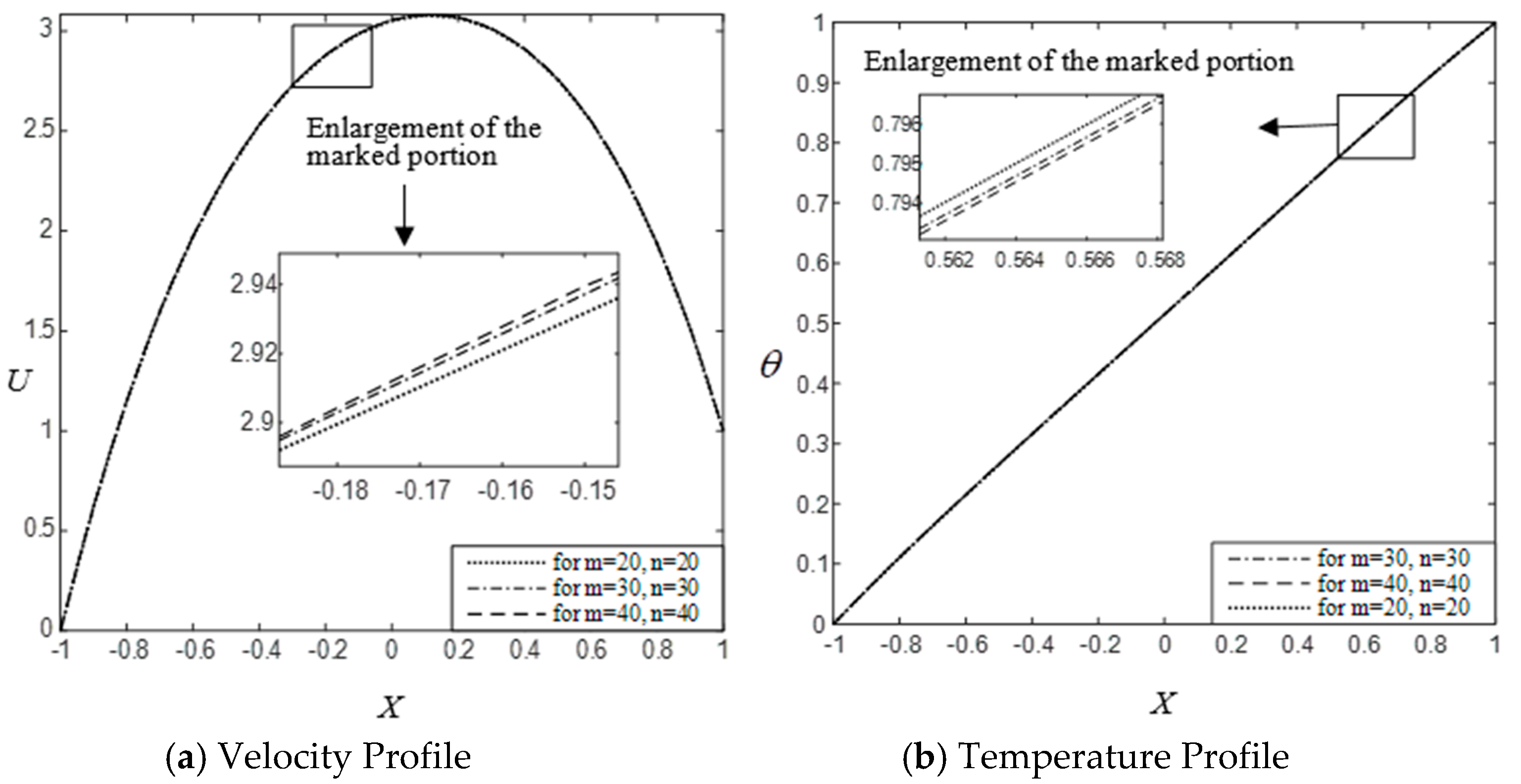
To obtain the appropriate grid space for $m\mathrm{and}n$ the computations have been carried out for three different grids, $\left(m=20,20\right);\left(m=30,30\right)\mathrm{and}\left(m=40,n=40\right)$, which are shown in Figure 3. It is seen from this figure that the graph for $\left(m=40,n=40\right)$ is more closed than others. Also it has been verified to enlarge the quoted point of the Figure 3a,b. The enlargement sub-figures of Figure 3a,b show that the dash and doted lines are closed to each other. Thus, $\left(m=40,n=40\right)$ can be chosen as the appropriate mesh. For further consideration, the results of velocity and temperature fields, shear stress, and Nusselt number have been simulated at $\left(m=40,n=40\right)$.

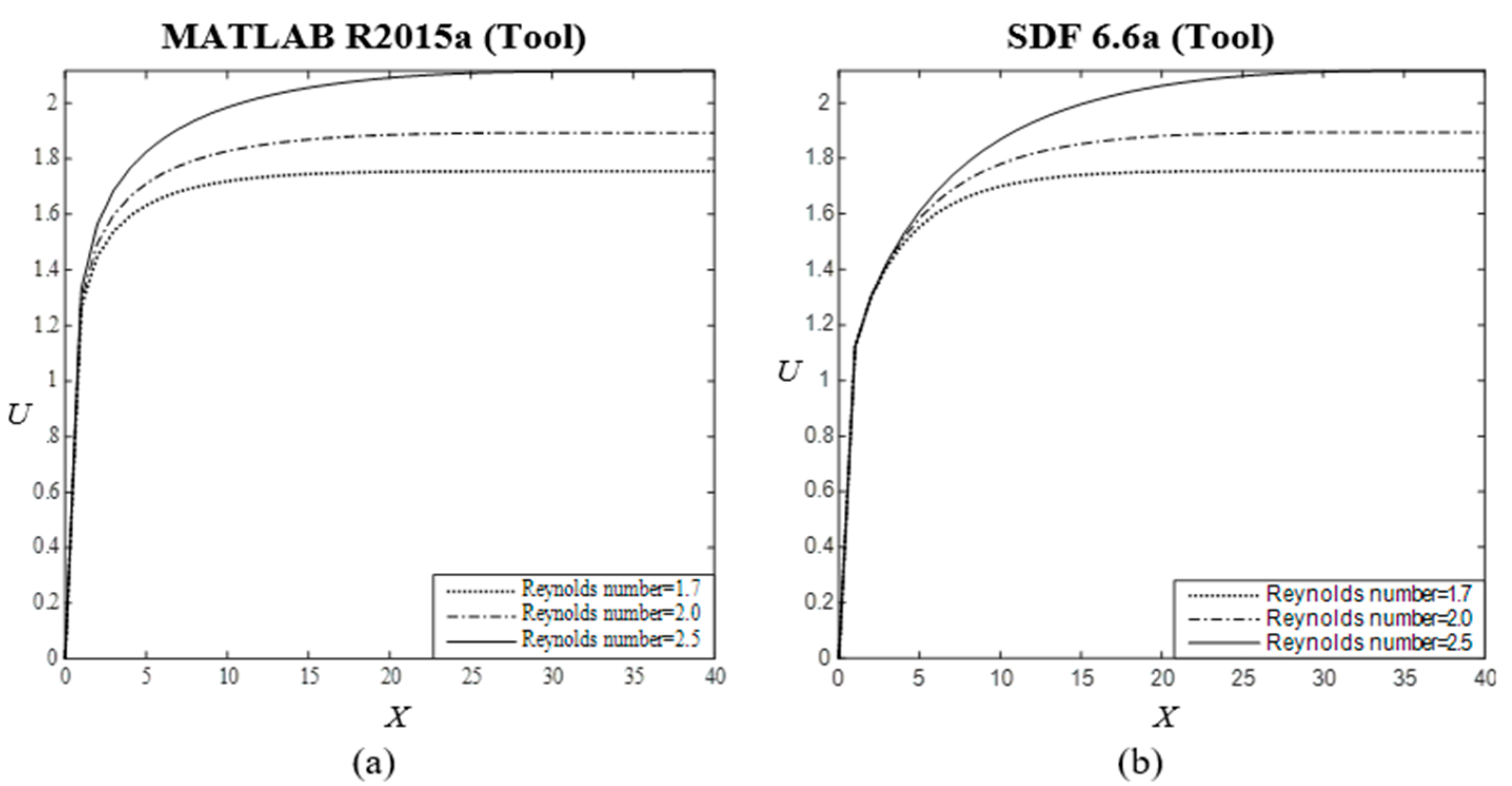
6.1.2. Sensitivity of MATLAB R2015a and SDF 6.6a

The accuracy is determined for the simulated results by MATLAB R2015a and SDF 6.6a tools and explicit finite difference is used as a solution technique. Using MATLAB and Fortran code, the Figure 4a,b are shown for velocity field and, Figure 4c,d are shown for the shear stress respectively. The impact of velocity field and shear stress at moving plate have been illustrated for several values of Reynolds number $\left(R_e\right)$. The identical results are obtained for both the tools (see Figure 4a–d). Thus, the sensitivity of coding achieved accuracy.

6.2. Steady-State Solution:

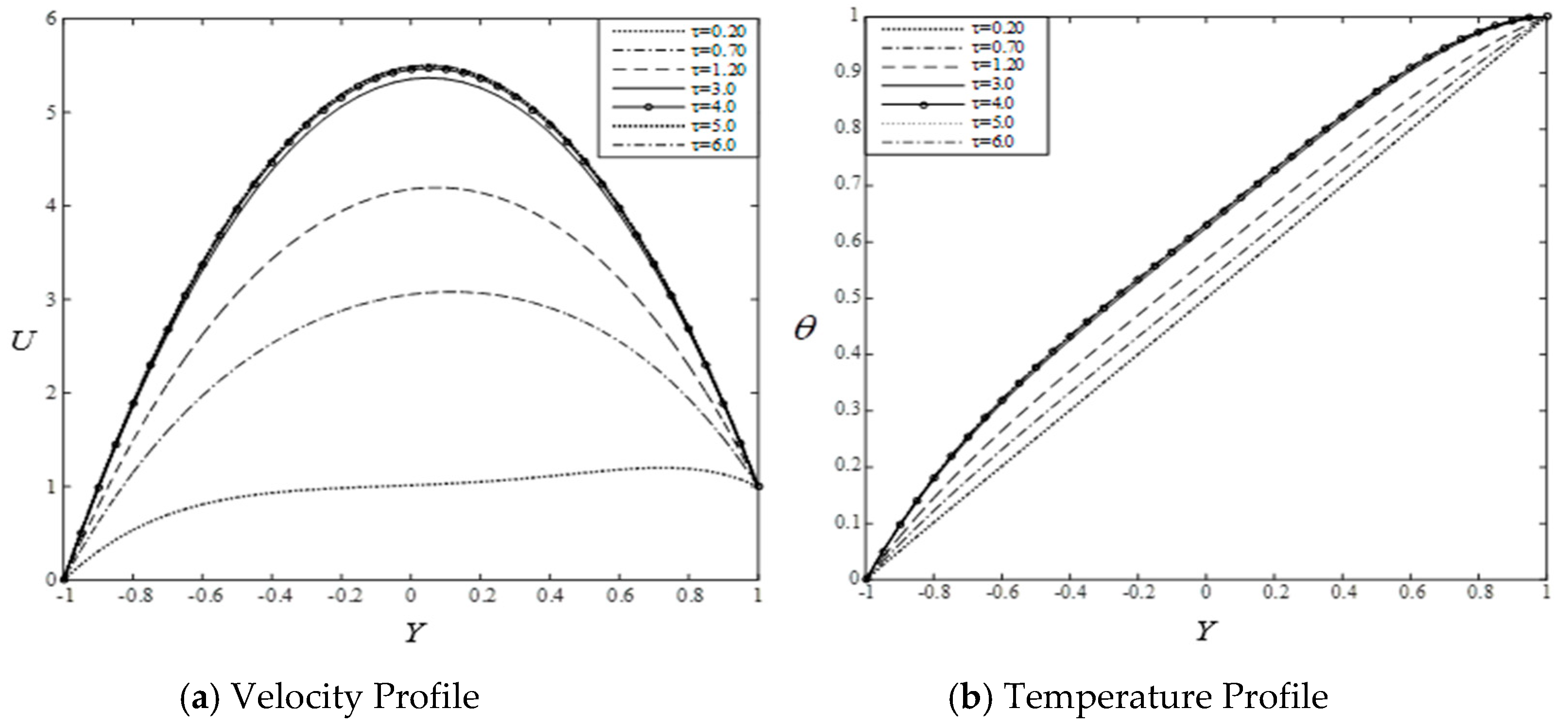
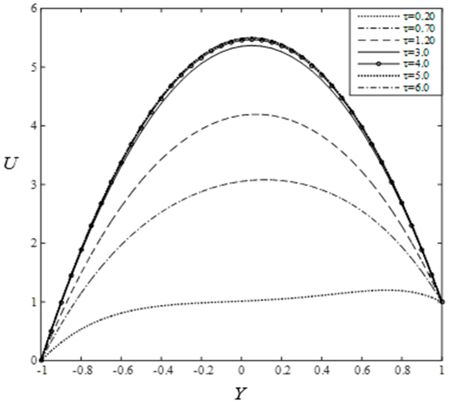
To acquire the steady-state solution of this developed mathematical model, the computations for velocity and temperature have been continued for different dimensionless times, such as $\tau =$ 0.20, 0.70, 1.20, 3.00, 4.00, 5.00, 6.00, etc. It is shown in Figure 5a,b that the computations for $U\mathrm{and}\theta$ have shown little change after $\tau =$ 3.00 and also shown negligible change after $\tau =$ 4.00. Thus, the solutions of all variables for $\tau =$ 4.00 are taken essentially as the steady-state solutions. Figure 5a,b show that the both velocity filed and temperature field attain steady-state monotonically. It also should be noted that the temperature profiles are reached steady state position than the velocity profiles.

6.3. Effects of Parameters:

To attain the clear conception of physical properties of the present study, the impact of parameters, namely Reynolds number $R_e$ and Bingham number ${\tau }_D$ on velocity and temperature, shear stress and Nusselt number at Prandtl number $\left(P_r=0.08\right)$ and Eckert number $\left(E_c=0.10\right)$ are illustrated in Figure 6 and Figure 7. For brevity, the impact of Prandtl number $P_r$ and Eckert number $E_c$ are not shown.

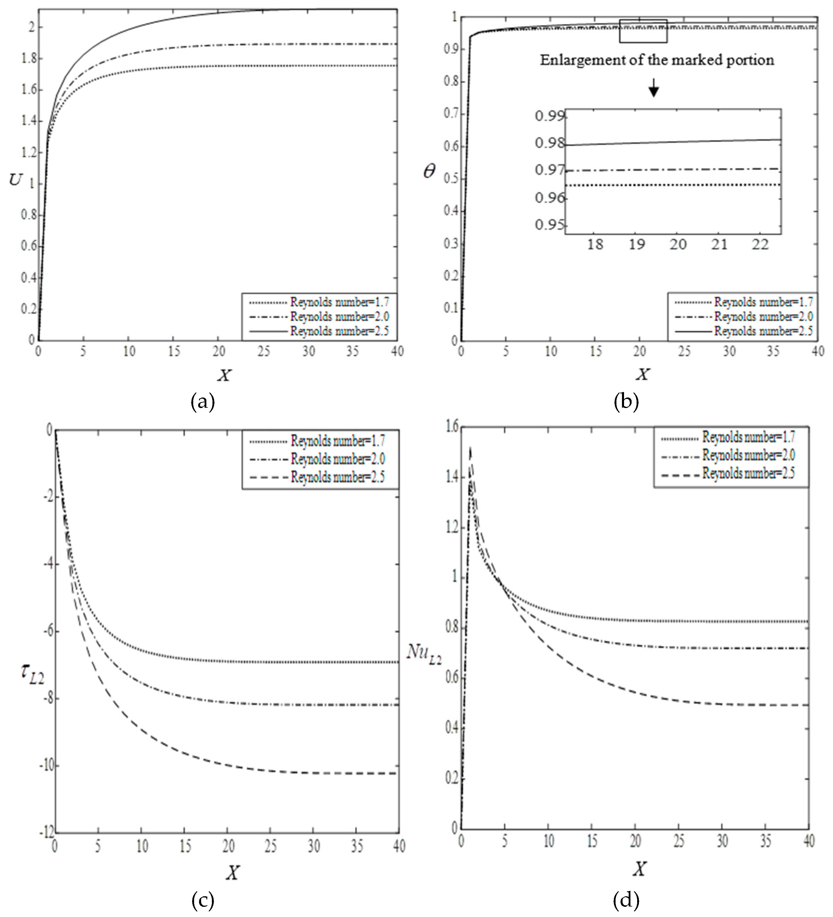
The influence of Reynolds number $R_e$ on velocity field, temperature field, shear stress and Nusselt number at moving plate are shown in Figure 6a–d. It is seen from Figure 6a,b, the velocity and temperature distributions decrease with the increase of Reynolds number $R_e$. Also it is seen from Figure 6b that the temperature distribution has minor decreasing effect. It has been checked to observe the effects by enlargement of the marked point on the curves of Figure 6b. The enlarge sub-figure of Figure 6b shows clearly the minor decreasing effects. It is observed from Figure 6c,d that both the shear stress and the Nusselt number at moving plate reduce with the increment of Reynolds number $R_e$.

The effects of Bingham number ${\tau }_D$ on velocity field, temperature field, shear stress and Nusselt number at moving plate are shown in Figure 7a–d. It is observed from Figure 7a,b that both the velocity and temperature distribution at moving plate enhance with the increment of Bingham number ${\tau }_D$. To check clearly the effects of velocity and temperature field, it has been enlarged the marked point of the curved of Figure 7a,b. The enlarged figures show clearly the enhancement of velocity and temperature fields.

It is observed from Figure 7c,d that both the profiles of the shear stress and the Nusselt number at moving plate enhance with the increment of Bingham number ${\tau }_D$. It has been checked to observe the effects by enlargement of the marked point on the curves of Figure 7c,d respectively. The enlarge sub-figures of Figure 7c,d show the minor decreasing effects clearly.

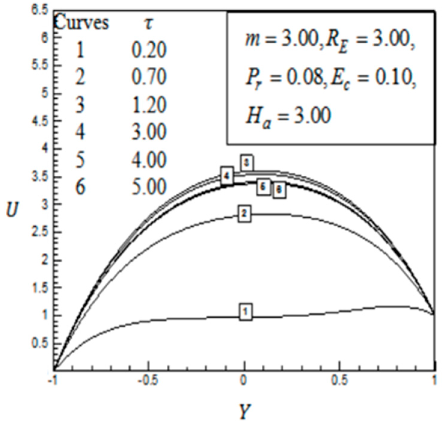
6.4. Comparison

Finally, qualitative and quantitative comparison of the study subject to the published results of Parvin et al. [8] are discussed in Figure 8 and Figure 9.

Thus, in Figure 8 and Figure 9, the obtained results are quantitatively not identical but quite similar qualitatively with the published results of Parvin et al. [8]. The problem has been solved numerically by explicit FDM. Since the present estimation has been verified by SDF 6.6a and MATLAB R2015a both software. Hence, our model is less flawed concerning published results.

7. Conclusions

In this study, the unsteady viscous incompressible Bingham fluid flow through a non-conducting parallel plate has been investigated numerically by explicit finite difference method. The physical properties are illustrated graphically for several values of Reynolds number $\left(R_e\right)$ and Bingham number $\left({\tau }_D\right)$. For brevity, the impact of Prandtl number $\left(P_r\right)$ and Eckert number $\left(E_c\right)$ are not shown. Some of the important observations from the graphical illustration of the presented results are listed below.

• The velocity and temperature fields rise with the increase of $R_e$.
• The velocity and temperature fields reduce with the increment of ${\tau }_D$.
• The shear stress and Nusselt number reduce with the increment of $R_e$.
• The shear stress and Nusselt number rise with the increment of ${\tau }_D$.
• The temperature reaches the steady-state quickly with the comparison of velocity distribution.