Two sets of experiments were conducted. The goal of the first set of experiments was to calibrate key parameters of algorithms running on the local controller (Marlin) and cloud-based controller. The second set of experiments was conducted to evaluate the performance of the cloud-based controller (in comparison with that of the local controller) using the parameters determined from the first set of experiments.
3.1. Calibration Experiments
The local controller (Marlin) runs a trapezoidal-speed motion command generator, which allows for limited-acceleration but infinite-jerk motion commands. In addition, it has a parameter known as jerk speed, which is a speed threshold below which motion commands are generated with infinite acceleration. A common practice is to tune the acceleration limit and jerk speed values iteratively to obtain the highest values that do not lead to excessive vibration of a given 3D printer. This allows the printer to travel as fast as possible while maintaining acceptable print surface quality (i.e., surfaces with minimal vibration marks, also known as ringing).
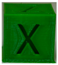
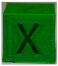
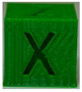
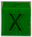
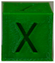
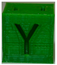
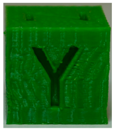
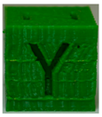
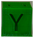
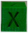
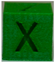
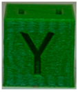
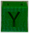
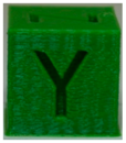
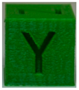
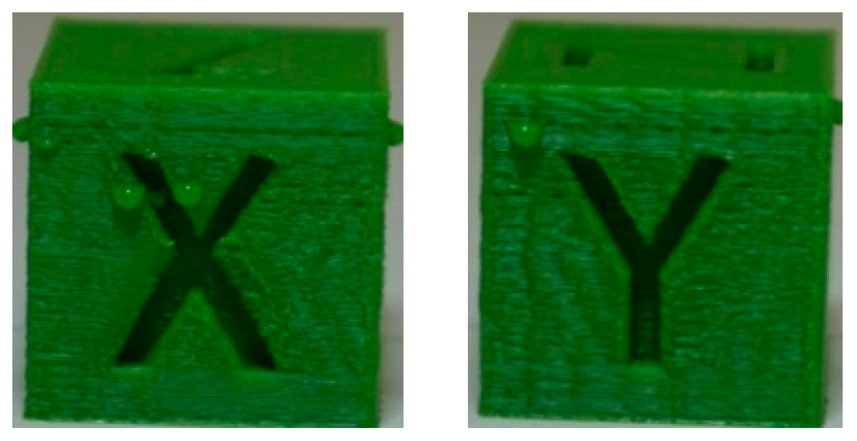
A very common artifact used for determining acceptable acceleration and jerk speed limits on desktop 3D printers like the Lulzbot Taz 6 is the XYZ Calibration Cube (with 20 mm sides), shown in
Figure 5. The sudden changes of motion direction at the edges of the cube and at the X and Y imprints on the faces of the cube excite vibration along the X and Y axes of the printer, leading to ringing on the faces of the cube.
Table 1 provides the key parameters used in all tests presented in this paper for slicing the calibration cube in Cura (Lulzbot Edition 21.04).
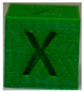
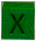
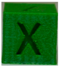
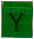
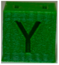
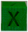
The first rows of
Table 2 and
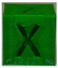
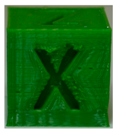
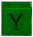
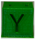
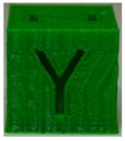
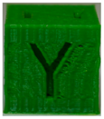
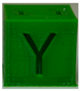
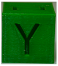
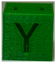
Table 3 respectively show the X and Y faces of the Calibration Cube printed using the local controller (i.e., Marlin running on the RAMBo board). Note that the cube is arbitrarily printed with its X-face aligned with the Y-axis, and is Y-face aligned with the X-axis of the Taz 6. All prints using the local controller are made with the default jerk speed of the Taz 6 printer (i.e., 10 mm/s). Notice that with the default acceleration limit of the printer (i.e., 0.5 m/s
2), the quality of the faces is generally okay, though each face has some ringing, with the X-face exhibiting a bit more ringing than the Y-face. As the acceleration limits are raised to 1, 5, and 10 m/s
2, the ringing steadily intensifies leading to increasingly worse surface quality, even though printing time progressively decreases.
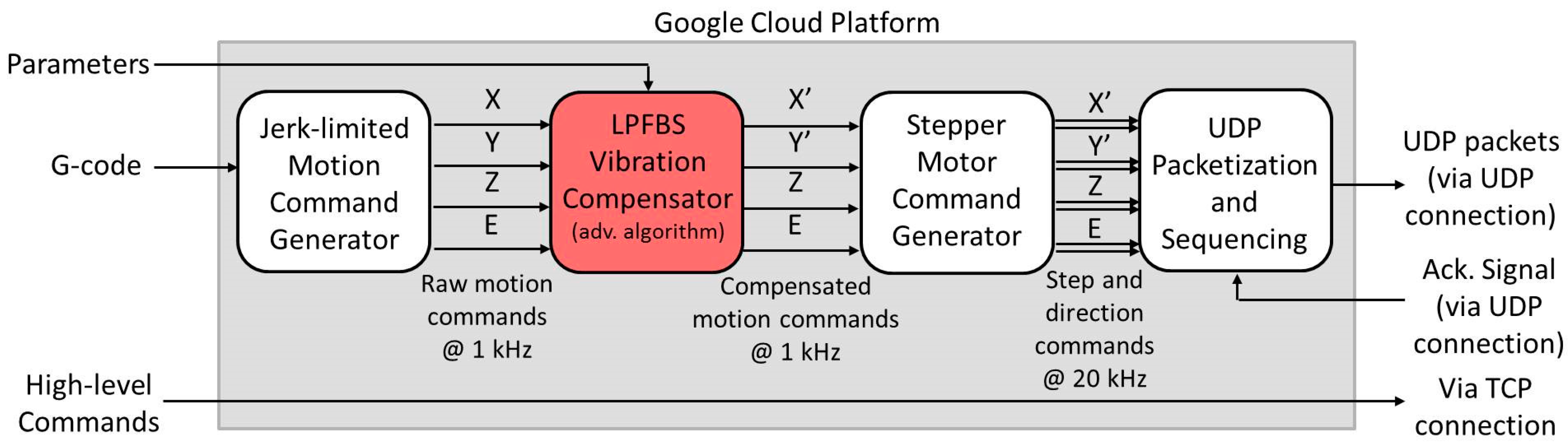
The cloud-based controller has two algorithms which together help to reduce vibration. First it uses a jerk-limited motion command generation (JLMCG) algorithm (also known as S-curve speed profile) [
30] which allows limitations on both acceleration and jerk. Moreover, it adds on the limited-preview filtered B-spline (LPFBS) algorithm [
31] which modifies motion commands to minimize vibration based on measured vibration dynamics of the printer. For the sake of the calibration tests, both algorithms (together with the stepper motor command generator in
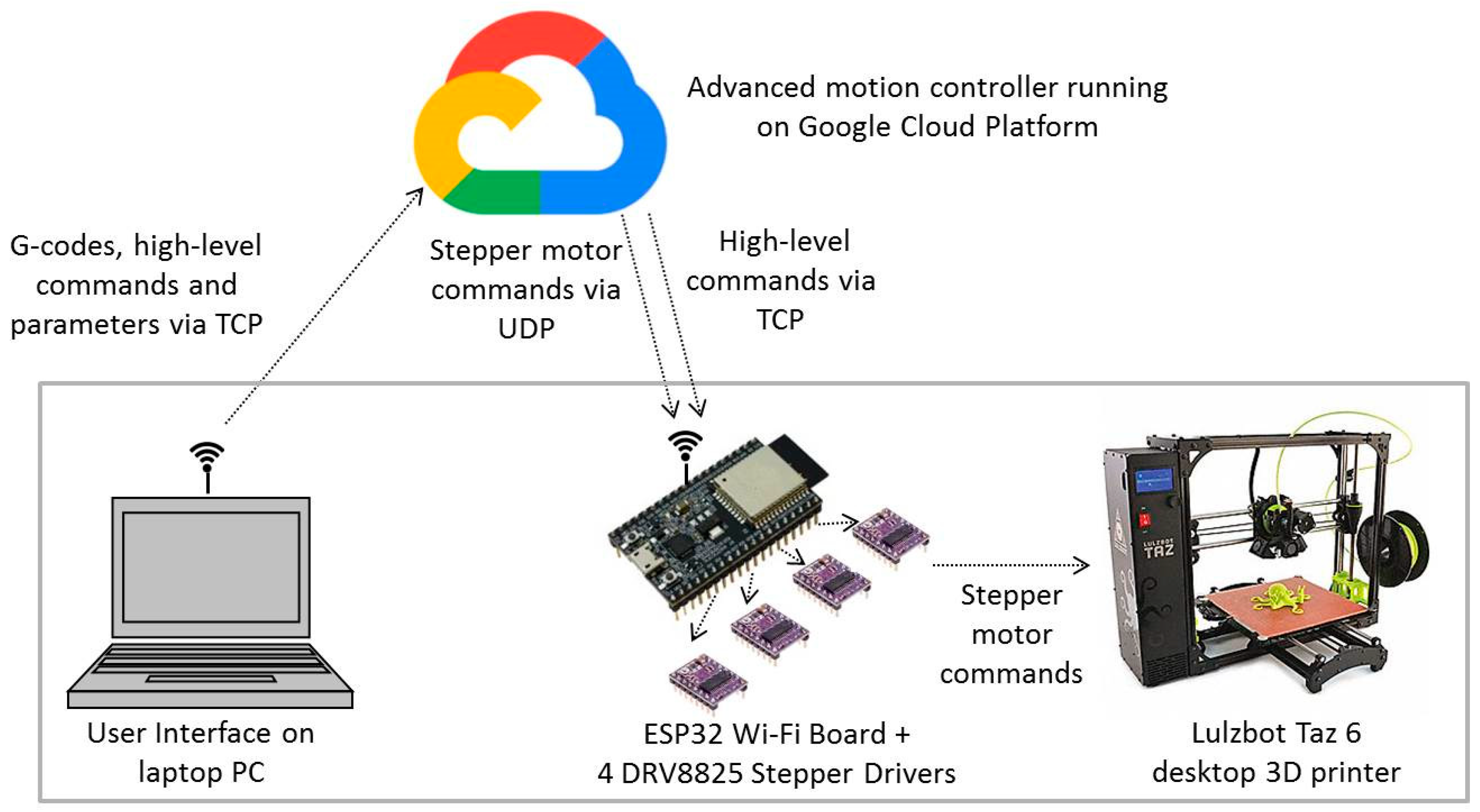
Figure 3) are implemented on the dSPACE DS1007 real-time control board running at 40 kHz clock frequency. The step and direction signals are sent via a wired connection at 13.33 kHz frequency to four DRV8825 stepper drivers connected to the X, Y, Z and E motors of the Taz 6 printer. In other words, the algorithms are implemented locally on a high-end motion control board with sufficient computational resources to run the LPFBS algorithm.
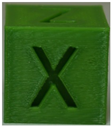
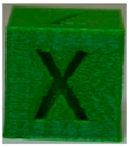
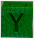
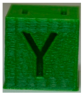
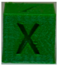
The second rows of
Table 2 and
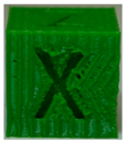
Table 3, respectively, show the effects of JLMCG on the X- and Y-faces of the calibration cube. The jerk limit is set at 5000 m/s
3, and acceleration limits of 0.5, 1, 5, and 10 m/s
2 are tested. Notice the improvements in surface quality compared to the local controller, though at the expense of longer printing time in each case due to the fact that both acceleration and jerk were limited.
To execute the LPFBS algorithm, the vibration dynamics of Taz 6 must be measured in the form of frequency response functions (FRFs) and modeled mathematically (see Reference [
31] for details).
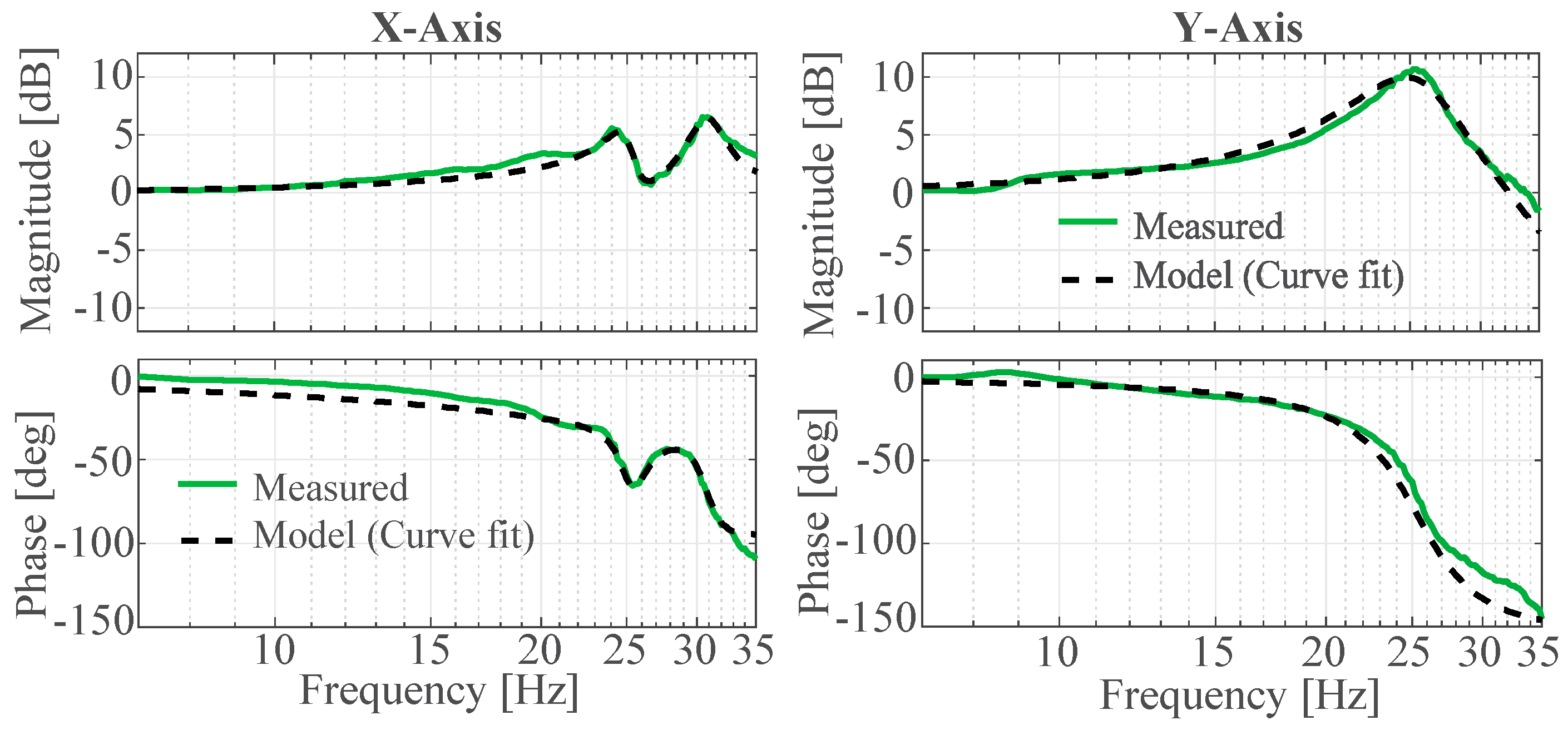
Figure 6 shows the measured and modeled FRFs of the X- and Y-axes of the Taz 6; the input of each FRF was acceleration commands to the corresponding stepper motor, and the output was relative acceleration between the build plate and nozzle in that direction, measured using accelerometers. The resulting transfer functions of the X and Y axes are given by Equations (1) and (2), respectively.
The slight discrepancies seen in
Figure 6 between the measured and modeled (curve fit) FRFs at low and high frequencies are due to the fact that the fitting is weighted to more accurately match dynamics around the resonance peaks, at the expense of dynamics at lower and higher frequencies. This is because the dynamics around the resonance frequencies are most influential on the vibration of the printer.
Table 4 summarizes other key parameters needed for implementing the LPFBS algorithm, following the detailed description and the exact same notations as used in Reference [
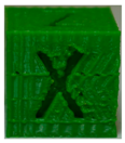
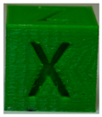
31]. The third rows of
Table 2 and
Table 3 respectively show the effects of JLMCG and LPFBS on the X and Y-faces of the Calibration Cube. Notice the significant improvements in surface quality at each acceleration level (without increasing the printing time relative to those of JLMCG alone).
Looking at the X-face of the cube, which is generally worse than the Y-face in terms of vibration marks, the quality of the 10 m/s2 case of JLMCG and LPFBS is at least as good as, if not better than, that of the local controller at its default 0.5 m/s2 acceleration limit. Therefore, in the following experiments, an acceleration limit of 0.5 m/s2 and jerk speed of 10 mm/s were used for the local controller while an acceleration limit of 10 m/s2 and jerk limit of 5000 m/s3 were used for the cloud-based controller (which runs both JLMCG and LPFBS).
3.2. Comparison of Local Controller with Cloud-Based Controller
Using the results of the calibration performed in the preceding section, two parts are printed using the cloud-based controller and compared with the same parts printed using the local controller (Marlin). The cloud-based controller was run on Google Compute Engines in two geographical locations—Moncks Corner, South Carolina and Sydney, Australia.
Table 5 provides specifications of the VMs at each location. The first location was selected to be sufficiently close to Michigan, where the printer was located, while the second location was selected to be as far as possible away from Michigan.
The first part printed was the Calibration Cube of
Figure 5. Four samples of the cube were printed from each location.
Table 6 and
Table 7 compare key attributes of the prints from the South Carolina and Australia-based controllers, respectively. For all four trials, the South Carolina-based controller ran hitch free, without any pauses due to latency. As a result, it returned prints with consistent printing times and similar surface quality as the corresponding part printed using dSPACE. Interestingly, the printing times of the South Carolina-based controller are about one minute shorter than that from dSPACE (see
Table 2 and
Table 3). This is due to slight differences in the implementation of the algorithms on dSPACE and the VMs. The dSPACE is a real-time computer which was run at a fixed 40 kHz clock frequency. The clock frequency was down-sampled by a factor of three to create each step for the stepper motors in real time at 13.33 kHz, and by a factor of 40 to generate the outputs of the JLMCG and LPFBS algorithms in real time at 1 kHz. On the other hand, the VMs are non-real-time computers. They ran the JLMCG and LPFBS algorithms at a sampling frequency of 1 kHz (non-real-time) and then up-sampled the output to 20 kHz stepping frequency. The non-real-time nature of the VMs provides more flexibility in the implementation of the algorithms (allowing up-sampling rather than down-sampling), leading to fewer approximations hence reductions in printing time.
A bit different from the South Carolina-based controller, the Australia-based controller experienced two short pauses due to internet delays during the first trial print, but the other three trials ran hitch free. As a result, the printing time for time for first trial was 19 s longer than those of the other three trials. However, the pauses did not have any noticeable effect on the surface quality of the first trial part. During each print, the round-trip time (RTT) was logged at regular intervals. The RTT measures the duration between sending a signal via internet protocol and getting an acknowledgement of its reception, and is commonly used as a measure of internet transmission- induced delays. Notice that the average and maximum RTT were significantly higher for the Australia-based controller compared to the South Carolina-based controller, in large part due to the longer distances traveled by the signals. Moreover, the first trial on the Australia based controller exhibited slightly higher average RTT than the other three trials; its peak RTT was also slightly higher than the others, though trial 3 had the largest peak RTT.
To compare the cloud-based controller to the local controller on a more involved print, the Medieval Castle model shown in
Figure 7 was sliced in Cura using the parameters reported in
Table 8. It was printed using the default parameters of the local controller (i.e., 0.5 m/s
2 acceleration and 10 mm/s jerk speed), as well as using the cloud-based controller hosted in South Carolina and Australia with 10 m/s
2 acceleration and 5000 m/s
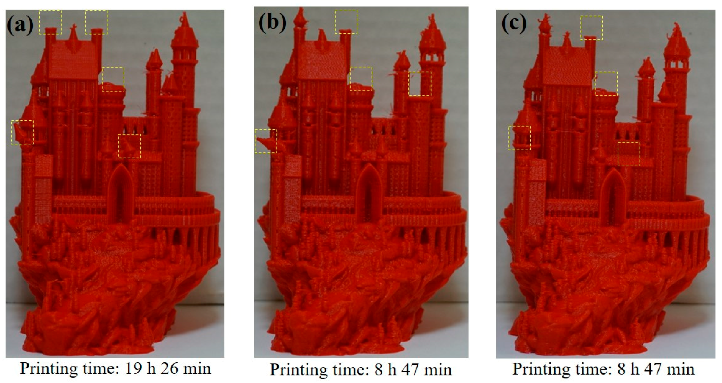
3 jerk limits. The results are shown in
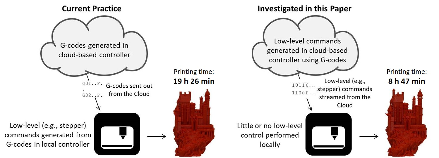
Figure 8. The local controller completed the print in 19 h 26 min while the cloud-based controller in South Carolina and Australia both completed it in 8 h 47 min, without any pauses throughout the prints. Note that the Castle could not be printed via dSPACE because of memory limitations; the G-code file for the Castle is 20 MB in size and could not be loaded into the memory of the dSPACE system for real-time execution. However, a PC-based MATLAB Simulink emulator, which predicts the printing time of the algorithms running on dSPACE accurately to the order of milliseconds, calculated a printing time of 9 h 27 min for the Castle. Therefore, the printing time of the cloud-based controller would have beaten that of the dSPACE system by 40 min (7%). Moreover, the memory limitations of the dSPACE system highlight the potential benefit of cloud-based controllers (whose memory requirements can be provisioned as need be).
In terms of printing accuracy, the prints by the local and cloud-based controllers are very similar. Notice that the local and cloud-based controllers alike failed in printing a few features at the top of some towers of the castle, highlighted by dashed yellow rectangles in
Figure 8. Those features broke off during printing due to very delicate support structures, and may need to be printed at feedrates much lower than 75 mm/s on both the local and cloud-based controllers. However, printing just those delicate portions at lower feedrates is not likely to affect overall printing time very significantly.


