The Zeta Filter: Attitude Estimation Using Von Mises–Fisher Concentration Dynamics on S³

Abstract

This paper presents an attitude filter that encodes both orientation and uncertainty in a single four-dimensional vector, requiring no covariance propagation or normalization constraints. The filter state is the natural parameter of the von Mises–Fisher (vMF) distribution on S³, whose exponential family structure reduces measurement updates to vector addition. Prediction is governed by a continuous-time ODE (Ordinary Differential Equation) that couples rotational kinematics with concentration decay. The QUEST-based construction of measurement natural parameters with a Fisher-information-matched concentration, an antipodal switching mechanism for the quaternion double cover, and a global exponential convergence analysis of the attitude error are described. The filter construction is left-invariant: it commutes with rotations of the reference frame, making the error dynamics trajectory-independent. The result is a filter with the computational simplicity of a complementary filter and the statistical grounding of Bayesian vMF fusion, operating entirely in unconstrained ℝ⁴ space. The filter is validated in simulation, on two recorded flights—including an evaluation against an EFIS attitude reference—and its computational cost is measured down to on-target microcontroller cycle counts. Gyroscope bias estimation is not included and is left to future work.

1. Introduction

Modern control and navigation systems for Unmanned Aerial Vehicles (UAVs) require precise and real-time attitude estimation [1,2,3,4,5,6]. Reliable attitude information underpins UAV applications well beyond inner-loop control, from flight-attitude determination for radar-based remote sensing [7] to endurance-oriented platforms whose stringent energy budgets leave little computational headroom [8]. Due to the limited computational resources of microcontrollers used in Inertial Measurement Units (IMUs) and the diverse dynamic states encountered during flight, selecting an appropriate estimation algorithm is a key design challenge.

Two groups of solutions currently dominate unmanned systems: complementary filters (e.g., Mahony or Madgwick) [9,10] and Extended Kalman Filters (EKF/MEKF) [11,12,13]. Complementary filters are valued for their low computational power requirements, making them ideal for small and less technologically advanced drones; however, they lack a built-in statistical measure of estimation uncertainty. In contrast, Kalman filters offer a rigorous statistical approach and error covariance tracking, but their implementation involves a high computational cost and the need for troublesome linearization on rotation manifolds.

Beyond these two families, a third line of work represents attitude uncertainty with probability densities on manifolds such as $SO\left(3\right)$ or its double cover $S^3$. These methods require normalization constraints, local parameterizations, or linearization in tangent spaces, increasing complexity. Filters like the matrix Fisher filter on $SO\left(3\right)$ [14], the unscented von Mises–Fisher filter [15], and the quaternion Bingham filter [16] show that exponential distribution family distributions on rotation groups enable additive Bayesian fusion in the natural parameter space. However, these filters use matrix-valued parameters and often require sigma-point propagation, moment matching, or decoupling the mean direction and concentration parameter, which raises computational cost and hinders real-time estimation. Tronarp et al. [17] derived exact continuous-time concentration dynamics for the vMF distribution on $S^2$, involving modified Bessel function ratios. This work applies the high-concentration asymptote of that result to $S^3$.

This article presents the concept of the Zeta filter, an original solution that can bridge the gap between the aforementioned classes of algorithms. The novelty of the filter is the definition of its state in the unconstrained quaternions set $\mathbb{H}$, which embeds both attitude and error model in a four-element vector, enabling extremely compact representation of the estimate. For UAV systems, the Zeta filter offers the following benefits:

• High computational efficiency: in the scenarios evaluated, its accuracy approaches that of the MEKF—a higher-class estimator that remains the accuracy reference when its noise assumptions hold—at a computational cost in the class of the simple complementary filters, measured at 1.8× the Mahony filter and an order of magnitude below the MEKF (Section 3.1.9);
• Global stability: Section 2.5 proves convergence from any initial attitude, including a 180° at a uniform exponential rate, under the standard two-vector observability assumption that the reference directions remain bounded away from collinearity. The recovery speed is uncertainty-scaled rather than gain-driven: the same mechanism that accelerates recovery when confidence is low does not amplify measurement disturbances during confident tracking, and no guarded initialization or recovery logic is required;
• Frame invariance: the filter commutes with rotations of the reference frame (left-invariance, Section 2.5), so its error behavior is trajectory-independent—the convergence rate proved in Section 2.5 holds uniformly over maneuvers.

The remainder of this article develops the filter and its theory: Section 2.1 and Section 2.2 define the natural parameter on $S^3$ and its connection to the von Mises–Fisher distribution; Section 2.3, Section 2.4 and Section 2.5 present the continuous-time prediction model, the additive measurement update, and the stability and convergence analysis; and Section 3.1 validates the filter against Mahony, Madgwick and MEKF baselines, in simulation and on recorded flight data.

2. Materials and Methods

2.1. The Natural Parameter on S³

In scalar Gaussian estimation, the concept of information fusion can be illustrated with the property that precision, defined as $1/{\sigma }^2$ (the inverse of the variance), is additive: $1/{\sigma }_{\mathit{post}}^2=1/{\sigma }_1^2+1/{\sigma }_2^2$. An analogous property holds for the vMF distribution on the unit sphere: Bayesian fusion reduces to parameter addition. This parallel is central: the filter presented here has a state given by the vMF natural parameter, preserving the additive fusion property, but now in ${\mathbb{R}}^4$ for orientation.

Let $\mu \in S^3\subset \mathbb{H}$ denote a unit quaternion representing the mean orientation and let $\kappa \ge 0$ denote the concentration parameter of the vMF distribution. The natural parameter is defined as:

$$\zeta ≔\kappa \mu \in {\mathbb{R}}^4\simeq \mathbb{H}$$

(1)

This single object encodes both attitude and certainty:

• Magnitude: $‖\zeta ‖=\kappa$ is the concentration (higher values correspond to tighter clustering around the mean direction)
• Direction: $\zeta /‖\zeta ‖=\mu$ is the unit quaternion representing attitude

$\zeta$ serves simultaneously as both the mean and the concentration—in contrast to the Kalman filter and its information form, which carry the estimate and its covariance (or information matrix) as separate objects. Matrix-parameter filters on rotation groups, such as the matrix Fisher filter [14], also embed both in a single parameter, but at the cost of a matrix-valued state and per-step matrix decompositions; here the same coupling is carried by four numbers. In the high-concentration regime ($\kappa \gg 100$), the concentration is related to the per-axis attitude standard deviation ${\sigma }_{\theta }$ by $\kappa \approx 4/{\sigma }_{\theta }^2$: a rotation error of angle $\Theta$ corresponds to a quaternion space angle $\Theta /2$ under the double cover ($\theta =2\mathit{arccos}{q}_w$), so ${\zeta }^{\top }\mu =\mathit{cos}\left(\Theta /2\right)\approx 1-{\Theta }^2/8$ and the vMF density behaves as $\mathit{exp} \left(-\kappa {\Theta }^2/8\right)$, i.e., carries information $\left(\kappa /4\right)I_3$ in rotation-vector coordinates. $\zeta$ is therefore analogous to the Gaussian information state. The filter operates in this high-concentration regime throughout: across the update rates used in this work (16.7–100 Hz on flight data, 100 Hz in simulation), the closed-loop equilibrium concentration of Section 2.5 lies between roughly $5\times {10}^3$ and ${10}^5$, one to three orders of magnitude above the $\kappa \gtrsim 100$ validity threshold of the prediction model’s asymptotics (Section 2.3).

2.2. Connection to the Von Mises–Fisher Distribution

The vMF distribution is a member of the exponential family with density:

$$p\left(x;\zeta \right)\hspace{0.25em}\propto \hspace{0.25em}\mathit{exp} \left({\zeta }^{\top }x\right),\hspace{1em}\hspace{1em}x\in S^3$$

(2)

It is this exponential family property that drives the Zeta filter: the log-likelihood is linear in $\zeta$, so Bayesian fusion reduces to vector addition. The representation remains meaningful even when $\zeta = 0$: the distribution becomes uniform on $S^3$, representing complete uncertainty.

2.2.1. Bayesian Fusion via Natural Parameter Addition

Let two independent vMF-distributed observations have natural parameters ${\zeta }_1$ and ${\zeta }_2$. The vMF is an exponential family, so multiplying their likelihoods gives the combined density:

$$p\left(x;{\zeta }_1\right) p\left(x;{\zeta }_2\right)\hspace{0.25em}\propto \hspace{0.25em}\mathit{exp} \left({\left({\zeta }_1+{\zeta }_2\right)}^{\top }x\right).$$

(3)

The fused natural parameter is therefore ${\zeta }^{+}={\zeta }_1+{\zeta }_2$. The posterior remains vMF, since the vMF is its own conjugate prior for the mean direction $\mu$ when concentrations are known [18].

2.2.2. Attitude Extraction

The attitude estimate is recovered by normalizing the natural parameter:

$$q≔{\displaystyle \frac{\zeta }{‖\zeta ‖}}$$

(4)

This is simply the mean direction $\mu$ of the vMF distribution. No separate mean estimate is maintained—the attitude is read from the direction of $\zeta$ when required.

2.3. Continuous-Time Prediction Model

The evolution of the estimated state $\widehat{\zeta }$ under gyroscope-driven prediction combines rotational kinematics coupled with stochastic concentration dissipation.

Let ${\omega }_b={\left[{\omega }_{b,x},{\omega }_{b,y},{\omega }_{b,z}\right]}^{\top }\in {\mathbb{R}}^3$ denote the measured angular velocity in the body frame and let ${\sigma }_g^2$ (units: rad²/s) denote the continuous-time noise intensity of the gyroscope, such that the angular random walk variance grows as ${\sigma }_g^2 \Delta t$ over a time interval $\Delta t$.

2.3.1. Prediction Step

The continuous-time dynamics are given by:

$$\dot{\widehat{\zeta }}=\underset{\mathit{rotation}}{\underbrace{{\displaystyle \frac{1}{2}}\widehat{\zeta }\otimes {\overline{\omega }}_b}}\underset{\begin{array}{c}concentration\\ dissipation\end{array}}{\underbrace{-\gamma \left(\widehat{\zeta }\right) \widehat{\zeta }}}$$

(5)

where ${\overline{\omega }}_b={\left[0,{\omega }_{b,x},{\omega }_{b,y},{\omega }_{b,z}\right]}^{\top }$ is the angular velocity embedded as a pure quaternion. Note that the Hamilton convention ($ij = k$) is used with scalar-first ordering $q={\left[w,x,y,z\right]}^{\top }$. Under this convention, $q \otimes r$ composes the rotation $r$ followed by $q$. The state-dependent dissipation factor is:

$$\gamma \left(\widehat{\zeta }\right)=\alpha {\sigma }_g^2‖\widehat{\zeta }‖,\hspace{1em}\hspace{1em}\alpha ={\displaystyle \frac{2}{p-1}}$$

(6)

where $\alpha$ follows from the high-$\kappa$ asymptotics of the exact vMF concentration dynamics (see below), and $p$ is the ambient dimension of $S^{p-1}$.

Equivalently, in matrix form:

$$\dot{\widehat{\zeta }}={\displaystyle \frac{1}{2}}\Omega \left({\omega }_b\right) \widehat{\zeta }-\alpha {\sigma }_g^2‖\widehat{\zeta }‖ \widehat{\zeta }$$

(7)

where $\Omega \left({\omega }_b\right)$ is the $4 \times 4$ skew-symmetric matrix:

$$\Omega \left({\omega }_b\right)=\left[\begin{array}{cccc}0& -{\omega }_{b,x}& -{\omega }_{b,y}& -{\omega }_{b,z}\\ {\omega }_{b,x}& 0& {\omega }_{b,z}& -{\omega }_{b,y}\\ {\omega }_{b,y}& -{\omega }_{b,z}& 0& {\omega }_{b,x}\\ {\omega }_{b,z}& {\omega }_{b,y}& -{\omega }_{b,x}& 0\end{array}\right]$$

(8)

2.3.2. Interpretation

The prediction model consists of two terms:

• Rotation term: The skew-symmetric matrix $\Omega \left({\omega }_b\right)$ generates a unitary rotation that preserves $‖\widehat{\zeta }‖$. This term propagates the attitude estimate according to the gyroscope input.
• Dissipation term: The term $-\gamma \left(\widehat{\zeta }\right)\widehat{\zeta }$ reduces the magnitude of $\widehat{\zeta }$, representing the loss of concentration (increase in uncertainty) due to process noise. As opposed to classical EKF formulations where process noise adds to the covariance, here noise subtracts from the concentration—a natural consequence of working in the information domain.

2.3.3. Norm Dynamics

Taking the time derivative of $‖\widehat{\zeta }‖$ via the chain rule:

$${\displaystyle \frac{d}{dt}}‖\widehat{\zeta }‖={\displaystyle \frac{\widehat{{\zeta }^{\top }}\dot{\widehat{\zeta }}}{‖\widehat{\zeta }‖}}$$

(9)

Substituting $\dot{\widehat{\zeta }}={\displaystyle \frac{1}{2}}\Omega \left({\omega }_b\right)\widehat{\zeta }-\alpha {\sigma }_g^2‖\widehat{\zeta }‖ \widehat{\zeta }$:

$${\displaystyle \frac{d}{dt}}‖\widehat{\zeta }‖={\displaystyle \frac{{\widehat{\zeta }}^{\top }\left(\frac{1}{2}\Omega \left({\omega }_b\right)\widehat{\zeta }-\alpha {\sigma }_g^2‖\widehat{\zeta }‖ \widehat{\zeta }\right)}{‖\widehat{\zeta }‖}}={\displaystyle \frac{\frac{1}{2}{\widehat{\zeta }}^{\top }\Omega \left({\omega }_b\right)\widehat{\zeta }-\alpha {\sigma }_g^2‖\widehat{\zeta }‖ {‖\widehat{\zeta }‖}^2}{‖\widehat{\zeta }‖}}$$

(10)

Since $\Omega \left({\omega }_b\right)$ is skew-symmetric, ${\widehat{\zeta }}^{\top }\Omega \left({\omega }_b\right)\widehat{\zeta }=0$, this equals:

$${\displaystyle \frac{d}{dt}}‖\widehat{\zeta }‖=-\alpha {\sigma }_g^2{‖\widehat{\zeta }‖}^2$$

(11)

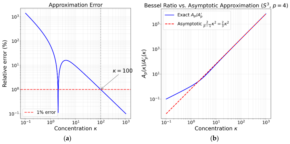
This is the high-$\kappa$ asymptote of the exact vMF concentration dynamics. The exact form, derived by Tronarp et al. [17] on $S^2$, involves the Bessel function ratio $A_p\left(\kappa \right)=I_{p/2}\left(\kappa \right)/I_{p/2-1}\left(\kappa \right)$: $\dot{\kappa }=-{\gamma }^2{A}_p\left(\kappa \right)/A_p^{\prime }\left(\kappa \right)$. The standard asymptotic expansion of modified Bessel functions gives $A_p\left(\kappa \right)\approx 1-\left(p-1\right)/\left(2\kappa \right)$ for large $\kappa$, so $A_p^{\prime }\left(\kappa \right)\approx \left(p-1\right)/\left(2{\kappa }^2\right)$ and:

$${\displaystyle \frac{A_p\left(\kappa \right)}{A_p^{\prime }\left(\kappa \right)}}\approx {\displaystyle \frac{2{\kappa }^2}{p-1}}=\alpha {\kappa }^2$$

(12)

yielding $\dot{\kappa }=-\alpha {\gamma }^2{\kappa }^2$ with $\alpha =2/\left(p-1\right)$. On $S^2$ ($p=3$), $\alpha = 1$ and the factor vanishes; on $S^3$ ($p=4$), $\alpha = 2/3$. In terms of the inverse concentration $v=1/\kappa$ the decay law reads $\dot{v}=\alpha {\sigma }_g^2$: linear growth of the vMF counterpart of variance, exactly as the variance of a Gaussian random walk grows linearly in the covariance domain. Figure 1 confirms that the asymptotic approximation is accurate to within 1% for $\kappa > 100$. This threshold is comfortably respected in closed-loop operation: the predict–update cycle holds the concentration near its equilibrium ${\kappa }_{eq}$ (Section 2.5), which is of order $5\times {10}^3$–${10}^5$ for the sensor configurations of Section 3.1. Below the threshold—immediately after a zero-concentration start, for instance—the asymptote overestimates the decay rate, so the approximation errs on the conservative side, declaring more uncertainty than the exact dynamics would.

The solution to Equation (11) is:

$$‖\widehat{\zeta }\left(t\right)‖={\displaystyle \frac{‖\widehat{\zeta }\left(0\right)‖}{1+\alpha {\sigma }_g^2‖\widehat{\zeta }\left(0\right)‖t}}$$

(13)

2.3.4. Approximate Closed-Form Expression

For constant angular velocity ${\omega }_b$, the full nonlinear system does not admit an exact analytical solution due to the state-dependent dissipation $\gamma \left(\widehat{\zeta }\right)=\alpha {\sigma }_g^2\Vert \widehat{\zeta }$. However, over a short time step $\Delta t\ll 1/\left(\alpha {\sigma }_g^2‖\widehat{\zeta }‖\right)$, freezing $\gamma$ at its initial value ${\gamma }_0=\alpha {\sigma }_g^2\Vert \widehat{\zeta }\left(0\right)\Vert$ yields the approximate linear system

$$\dot{\widehat{\zeta }}\approx \left({\displaystyle \frac{1}{2}}\Omega \left({\omega }_b\right)-{\gamma }_{0}I\right)\widehat{\zeta },$$

(14)

with approximate solution:

$$\widehat{\zeta }\left(\Delta t\right)\approx \underset{\begin{array}{c}concentration\\ decay\end{array}}{\underbrace{e^{-{\gamma }_0\Delta t}}}\cdot \underset{\mathit{unitary} \mathit{rotation}}{\underbrace{e^{{\displaystyle \frac{1}{2}}\Omega \left({\omega }_b\right)\Delta t}}}\cdot \widehat{\zeta }\left(0\right).$$

(15)

For the exact norm evolution, the rational decay from the norm dynamics (above) should be used:

$$‖ \Delta t‖={\displaystyle \frac{‖\widehat{\zeta }\left(0\right)‖}{1+\alpha {\sigma }_g^2‖\widehat{\zeta }\left(0\right)‖ \Delta t}}$$

(16)

In practice, the direction may be propagated using the rotation matrix exponential, while the magnitude is updated using the exact rational decay, combining the best of both:

$$\widehat{\zeta }\left(\Delta t\right)={\displaystyle \frac{‖\widehat{\zeta }\left(0\right)‖}{1+\alpha {\sigma }_g^2‖\widehat{\zeta }\left(0\right)‖ \Delta t}}\cdot e^{{\displaystyle \frac{1}{2}}\Omega \left({\omega }_b\right)\Delta t}\cdot {\displaystyle \frac{\widehat{\zeta }\left(0\right)}{‖\widehat{\zeta }\left(0\right)‖}}$$

(17)

This form shows that the prediction step “remembers” the orientation while systematically losing certainty, exactly as in the physical intuition of gyroscope integration without correction.

2.4. Measurement Update

The measurement update follows directly from the natural parameter additivity of the vMF distribution established in Section 2.2. Given the a priori estimate ${\widehat{\zeta }}^{-}$ and measurement-derived ${\zeta }_{\mathit{obs}}$, the posterior is:

$$\boxed{{\widehat{\zeta }}^{+}={\widehat{\zeta }}^{-}+{\zeta }_{\mathit{obs}}}$$

(18)

This is exact Bayesian fusion within the vMF family—the posterior vMF distribution has natural parameter equal to the sum of the prior and likelihood natural parameters. No approximation or linearization is involved in the update rule itself.

2.4.1. Antipodal Selection

Since quaternions have the double-cover property ($q$ and $-q$ represent the same rotation in $SO\left(3\right)$), every measurement yields two valid natural parameter candidates: ${\zeta }_{\mathit{obs}}$ and $-{\zeta }_{\mathit{obs}}$. The filter resolves the issue by always selecting the candidate with the smaller angle to the prior:

$${\zeta }_{\mathit{obs}}\leftarrow \mathit{sign}\left({\widehat{\zeta }}^{-\top }{\zeta }_{\mathit{obs}}\right)\cdot {\zeta }_{\mathit{obs}}$$

(19)

This ensures ${\widehat{\zeta }}^{-\top }{\zeta }_{\mathit{obs}}\ge 0$ (angle $\le 90°$ in ${\mathbb{R}}^4$, corresponding to $\le 180°$ in $SO\left(3\right)$). This is always achievable because a $90°$ angle in quaternion space spans the full $180°$ rotation range—no physical rotation disagreement can exceed this limit.

The selection’s routine function is bookkeeping on the double cover. The QUEST solution carries a fixed sign convention (non-negative scalar part), confining ${\zeta }_{obs}$ to one closed hemisphere of $S^3$; the prior, by contrast, evolves continuously under the prediction ODE and crosses to the opposite hemisphere whenever the accumulated rotation carries it there—a continuous 360° rotation returns the attitude to its start while taking the quaternion from $q$ to $-q$. On such stretches ${\widehat{\zeta }}^{-\mathrm{T}}{\zeta }_{obs}$ is negative at every cycle even at a fraction of a degree of attitude disagreement, and (19) simply re-expresses each measurement on the prior’s current hemisphere: a deterministic relabelling with no possibility of chatter, since the prior moves continuously while the sign is re-derived afresh at each update (on the recorded flight of Section 3.1.7 it re-signs 24% of all updates without incident).

Genuine disagreement—between prior and measurement as rotations, after sign alignment—is a separate case and never approaches the 90° threshold in tracking: even 200°/s at the lowest update rate used (16.7 Hz, Section 3.1.8) advances the attitude by only 6° per cycle in ℍ, and an isolated corrupted measurement cannot flip the selection, its influence being bounded by the weight ratio ${\kappa }_{obs}/{\kappa }^{-}\ll 1$ of a single update. A stress test that feeds the filter adversarial near-antipodal streams (measurement errors alternating between +179° and −179°, and measurements placed exactly at the cut locus) confirms that the mechanism neither chatters nor stalls: after sign selection the alternating stream is internally consistent (the two errors are only 2° apart as rotations) and the estimate follows it smoothly, while even a maximally contradictory ±90° alternation merely holds the estimate steady until consistent measurements resume. Genuinely large disagreements arise only at initialization or recovery after divergence, where the selection enables the one-step exit from the antipode (Section 2.5).

Beyond the double-cover ambiguity, there is a more fundamental reason for this switching: the vMF distribution is not antipodally symmetric. $q$ and $-q$ correspond to opposite modes, and fusing the wrong sign would subtract rather than add concentration.

2.4.2. Properties of the Additive Update

• Concentration accumulation: Since antipodal selection secures ${\widehat{\zeta }}^{-\top }{\zeta }_{\mathit{obs}}\ge 0$, the posterior magnitude satisfies

$$\begin{gathered} {‖{\widehat{\zeta }}^{+}‖}^2={‖{\widehat{\zeta }}^{-}‖}^2+{‖{\zeta }_{\mathit{obs}}‖}^2+2 {\widehat{\zeta }}^{-\top }{\zeta }_{\mathit{obs}} \\ \ge {‖{\widehat{\zeta }}^{-}‖}^2+{‖{\zeta }_{\mathit{obs}}‖}^2 \end{gathered}$$

(20)

and therefore $‖{\widehat{\zeta }}^{+}‖\ge \mathit{max}\left(‖{\widehat{\zeta }}^{-}‖,‖{\zeta }_{\mathit{obs}}‖\right)$. When aligned, concentrations add:

$$‖{\widehat{\zeta }}^{+}‖=‖{\widehat{\zeta }}^{-}‖+\Vert {\zeta }_{\mathit{obs}}.$$

• Attitude averaging: The posterior direction ${\widehat{\zeta }}^{+}/‖{\widehat{\zeta }}^{+}‖$ is a concentration-weighted average of the prior and observation attitudes: the state moves along a straight segment in ℝ⁴, and its normalized direction moves along the great-circle arc from the prior toward the observed attitude, enabling large-angle corrections in a single update step.
• Zero-state recovery: If ${\widehat{\zeta }}^{-}=0$ (complete prior uncertainty), then ${\widehat{\zeta }}^{+}={\zeta }_{\mathit{obs}}$—the posterior is determined entirely by the measurement. This provides natural initialization without special cases and avoids division-by-zero errors in attitude extraction.

2.4.3. Construction of Measurement Natural Parameter

The measurement natural parameter ${\zeta }_{\mathit{obs}}$ is constructed from body-frame vector observations employing the QUEST (QUaternion ESTimator) algorithm [19]. This requires two vector measurements available at the same time—typically an accelerometer (gravity direction) and a magnetometer (magnetic field direction)—both sampled at the same rate.

Given $n = 2$ reference vectors $r_i$ in the world frame and corresponding body-frame measurements $b_i$ with associated weights $a_i$, QUEST solves Wahba’s problem [20] by finding the unit quaternion $q_{\mathit{obs}}$ that maximizes:

$$J\left(q\right)=\sum _{i=1}^n{a}_i b_i^{\top }R{\left(q\right)}^{\top } r_i$$

(21)

where $R\left(q\right)$ is the body-to-world rotation associated with the unit quaternion $q\in S^3$, consistent with the kinematic convention of Section 2.3 ($q\otimes r$ composing the rotation $r$ followed by $q$); equivalently the cost is maximized by aligning $R\left(q\right)b_i$ with $r_i$ (so $b_i\approx R{\left(q\right)}^{\top } r_i$ at the optimum).

The measurement natural parameter is then constructed as:

$${\zeta }_{\mathit{obs}}={\kappa }_{\mathit{obs}} q_{\mathit{obs}}$$

(22)

The measurement concentration must match the curvature of the measurement log-likelihood at its optimum, not its value: concentration is an information quantity, and information is the negative Hessian of the log-likelihood [21,22]. With the maximum-likelihood weights $a_i=1/{\sigma }_i^2$, the negative log-likelihood of the vector measurements is $-log L\left(q\right) = const - {\sum }_i{a}_i b_i^{T}R{\left(q\right)}^T{r}_i$, and its Hessian at $q_{obs}$, expressed in rotation-vector coordinates $\delta \theta$, is the classical QUEST Fisher information matrix [19,22]:

$$F=\sum _{i=1}^n{a}_i\left(I_3-{\widehat{b}}_i{\widehat{b}}_i^T\right),\hspace{1em}\hspace{1em}{a}_i={\displaystyle \frac{1}{{\sigma }_i^2}}$$

(23)

where ${\widehat{b}}_i$ are the unit body-frame measurements.

The vMF factor $exp({\kappa }_{obs} q^T{q}_{obs})$ expands for small rotation errors as $-log p \approx \left({\kappa }_{obs}/8\right){‖\delta \theta ‖}^2$, i.e., an isotropic information matrix $\left({\kappa }_{obs}/4\right)I_3$ (Section 2). $F$ is in general anisotropic, while a single vMF factor can only carry isotropic information, so a scalar reduction of $F$ must be chosen. The filter adopts the conservative (minimax) projection: the largest isotropic information matrix dominated by $F$ on every axis, $\left({\kappa }_{obs}/4\right)I_3⪯ F$, i.e.,

$${\kappa }_{obs}=4{\lambda }_{min}\left(F\right)$$

(24)

Mean-based reductions, such as Kullback–Leibler moment matching [23] (which yields the harmonic mean of the eigenvalues of $F$, $\kappa =12/tr\left(F^{-1}\right)$), overstate the information on the weakest axis whenever the eigenvalues are spread; since the weakest axis also dominates the attitude error, (24) is the largest weight that overstates none. Section 3.1.1 confirms the choice empirically: the grid-searched optimal weight coincides with (24) to within a few percent in both noise configurations.

For two vector observations, ${\lambda }_{min}$ has the closed form

$${\lambda }_{min}={\displaystyle \frac{1}{2}}\left[\left(a_1+a_2\right)-\sqrt{{\left(a_1+a_2\right)}^2-4a_1{a}_2{\mathit{sin}}^2\delta }\right]$$

(25)

with $\delta$ the angle between the unit measurements.

For a typical accelerometer–magnetometer pair, the weakest axis is yaw, ${\lambda }_{min}\approx a_m{\mathit{sin}}^2\delta$: ${\kappa }_{obs}$ is governed by the magnetometer weight $a_m$ and the reference vector separation $\delta$, and even with equal sensor noises, the attitude information remains anisotropic through the geometry alone (${\lambda }_{min}=a\left(1-\mathit{cos}\delta \right)$ versus $2a$ on the strongest axis). As the two reference vectors approach collinearity, ${\lambda }_{min}\to 0$ and ${\kappa }_{obs}\to 0:$ the observability degeneracy of the two-vector problem is handled gracefully, the measurement simply carrying no weight, with no special case required.

This construction is an assumed-density approximation: the true attitude information $F$ is anisotropic (Bingham-type), and a single vMF on $S^3$ retains only its weakest-axis isotropic reduction—the deliberate price of the scalar-concentration state.

The resulting update ensures that:

• ${\zeta }_{\mathit{obs}}$ is a valid vMF natural parameter with well-defined direction (attitude) and magnitude (concentration).
• No singularities arise at $\widehat{\zeta }=0$
• The update remains globally defined on ${\mathbb{R}}^4$

The construction is not limited to the accelerometer–magnetometer pair: (23) and (24) hold for any number n of vector observations, and by the additivity of the update any independent attitude-bearing source, such as a vision- or lidar-derived orientation, can contribute its own ${\zeta }_{obs}$ increment in the same cycle.

2.5. Stability and Convergence

2.5.1. Frame Equivariance

All three filter operations commute with a constant rotation of the reference frame. Represent such a rotation by left—translation $L_u\zeta =u\otimes \zeta$ with a fixed unit quaternion $u\in S^3$; note that $L_u$ is a linear map of ${\mathbb{R}}^4$ and, since $‖u\otimes \zeta ‖=‖\zeta ‖$, an orthogonal one. Relabeling the world frame by $R\left(u\right)$ sends the reference vectors $r_i\mapsto R\left(u\right) r_i$ while leaving all body-frame quantities $\left({\omega }_b,b_i,a_i\right)$ unchanged.

Each operation then carries the factor $u$ through unchanged. The rotational term of (7) is a right-translation, which commutes with $L_u$ by associativity, and the dissipation coefficient $\alpha {\sigma }_g^2‖\widehat{\zeta }‖$ is norm-invariant, so the prediction flow maps $L_u\widehat{\zeta }$ to $L_u\widehat{\zeta }$. The QUEST estimate transforms as $q_{obs}\mapsto u\otimes q_{obs}$, while the Fisher matrix $F=\sum _i{a}_i\left(I_3-{\widehat{b}}_i{\widehat{b}}_i^{\top }\right)$ and hence ${\kappa }_{obs}$ in (24) depend only on body-frame measurements and are unchanged. The sign selection (19) is invariant because $L_u$ preserves inner products, and the additive update (18) commutes with $L_u$ because $L_u$ is linear. Composing these over a predict–update cycle, and initializing at ${\widehat{\zeta }}_u\left(0\right)=u\otimes \widehat{\zeta }\left(0\right)$, gives

$${\widehat{\zeta }}_u\left(t\right)=u\otimes \widehat{\zeta }\left(t\right)\hspace{1em}\hspace{1em}\mathrm{for} \mathrm{all} t,$$

(26)

so the filter is left-invariant in the sense of invariant-observer theory [24]: relabeling the world frame maps filter trajectories to filter trajectories. The same argument applies to a fixed change in body frame (right-translation, under which $F$ undergoes a similarity that leaves its eigenvalues unchanged). Both properties are verified numerically to machine precision in the published simulation code.

2.5.2. Stability of the Prediction Dynamics

The prediction dynamics are shown to be globally asymptotically stable (GAS) toward the origin $\widehat{\zeta }=0$ using the Lyapunov criterion.

• Lyapunov function: Consider $V\left(\widehat{\zeta }\right)={‖\widehat{\zeta }‖}^2$. Taking the time derivative and substituting $\gamma \left(\widehat{\zeta }\right)=\alpha {\sigma }_g^2‖\widehat{\zeta }‖$:

$$\dot{V}=2{\widehat{\zeta }}^{\top }\dot{\widehat{\zeta }}=2{\widehat{\zeta }}^{\top }\left({\displaystyle \frac{1}{2}}\Omega \left({\omega }_b\right)\widehat{\zeta }-\alpha {\sigma }_g^2‖\widehat{\zeta }‖ \widehat{\zeta }\right)=-2\alpha {\sigma }_g^2{‖\widehat{\zeta }‖}^3<0$$

(27)

since ${\widehat{\zeta }}^{\top }\Omega \left({\omega }_b\right)\widehat{\zeta }=0$ (skew-symmetry) and $\alpha {\sigma }_g^2>0$ for $\widehat{\zeta }\ne 0$.

• Polynomial convergence: The norm satisfies the exact solution $‖\widehat{\zeta }\left(t\right)‖=‖\widehat{\zeta }\left(0\right)‖/\left(1+\alpha {\sigma }_g^2‖\widehat{\zeta }\left(0\right)‖t\right)$, demonstrating $O\left(1/t\right)$ decay to zero. This is slower than an exponential rate yet reflects the physically correct behavior: as concentration decreases, the rate of concentration loss also decreases (since there is less information left to lose).
• Global definition: The dynamics are globally defined on ${\mathbb{R}}^4$ with no singularities. The origin $\widehat{\zeta }=0$ represents complete uncertainty (uniform distribution over all orientations).

This stability result confirms that, in the absence of measurements, the filter correctly propagates toward maximum entropy. The uncertainty evolution is embedded directly in the state dynamics, eliminating the requirement for separate covariance propagation.

The same mechanism makes intermittent measurement loss—magnetometer interference or accelerometer saturation, for instance—benign: when no measurement is available, the update step is simply skipped and the filter runs on prediction alone, exactly as a Kalman filter coasts on its time update; the concentration decays toward the uniform prior over the outage, and the next valid measurement is fused with correspondingly greater relative weight. No special handling is required.

2.5.3. Convergence of the Concentration

The prediction dynamics drive $‖\widehat{\zeta }‖\to 0$, while measurement updates increase $‖\widehat{\zeta }‖$. The combined predict–update cycle is shown below to confine the concentration to an attracting band around a unique equilibrium.

Let measurements arrive at intervals $\Delta t$ with measurement concentration bounded as $0 < {\kappa }_{min} \le ‖{\zeta }_{obs}‖ \le {\kappa }_{max}$, and denote the prediction (rational-decay) map by $D\left(\kappa \right)=\kappa /(1+\alpha {\sigma }_g^2\kappa \Delta t)$. Because the antipodal selection of Section 2.4 guarantees ${\widehat{\zeta }}^{-T}{\zeta }_{obs} \ge 0$, the post-update norm is sandwiched for any attitude disagreement:

$$\sqrt{D{\left(\kappa \right)}^2+{\kappa }_{min}^2}\le {\kappa }^{+}\le D\left(\kappa \right)+{\kappa }_{max}$$

(28)

where the upper bound is attained for aligned fusion and the lower bound for orthogonal fusion. Both bounding maps are monotone increasing in $\kappa$ with a unique attracting fixed point (${\kappa }_{lo}$ and ${\kappa }_{hi}$ respectively; existence and uniqueness follow from the intermediate value theorem exactly as for the aligned map $g\left(\kappa \right) = D\left(\kappa \right) + {\kappa }_{max}$: the net change $h\left(\kappa \right)=g\left(\kappa \right)-\kappa$ satisfies $h\left(0\right)>0, h\to -\infty , h^{\prime } <0$). By monotone comparison, the concentration enters the invariant band $[{\kappa }_{lo}, {\kappa }_{hi}]$ and remains there, regardless of the attitude error along the way. Moreover, the rational decay imposes a trajectory-independent ceiling, $D\left(\kappa \right)<1/\left(\alpha {\sigma }_g^2\Delta t\right)$ for every $\kappa$, so after a single cycle

$${\kappa }^{+}\le {\kappa }_{hi}^{\ast }≔{\displaystyle \frac{1}{\alpha {\sigma }_g^2\Delta t}}+{\kappa }_{max}$$

(29)

uniformly in the initial condition—a consequence of the Riccati (quadratic) form of the dissipation. For small Δt the band collapses to the equilibrium concentration

$${\kappa }_{\mathit{eq}}\approx \sqrt{{\displaystyle \frac{{\kappa }_{obs}}{\alpha {\sigma }_g^2 \Delta t}}}$$

(30)

2.5.4. Convergence of the Attitude Error

The preceding result concerns only the scalar concentration. The quantity of practical interest is the attitude error, and the structure of the filter permits a global statement about it. The analysis follows the standard pattern of attitude-observer stability proofs—a Lyapunov function of the attitude error with a per-step contraction bound [9,25]—adapted to the discrete additive update and inherits its trajectory independence from the frame equivariance established above [24].

Define the quaternion-space misalignment $\tilde{\theta }$ between the true attitude $q\left(t\right)$ and the estimate direction by

$$\mathit{cos}\tilde{\theta }={\displaystyle \frac{q^T\widehat{\zeta } }{‖\widehat{\zeta } ‖}}$$

(31)

evaluated for the antipodal representative of $q$ chosen in Section 2.4; this makes $\mathit{cos}\tilde{\theta } \ge 0$, so $\tilde{\theta } \in [0, \pi /2]$, with the corresponding $SO\left(3\right)$ error $\tilde{\Theta }=2\tilde{\theta }$ covering the full range $[0, \pi ]$.

Prediction is error-neutral. With an exact gyroscope, the true quaternion and the estimate share the same rotational drive, $\dot{q}=\mathrm{½} q\otimes {\overline{\omega }}_b$ and $\dot{\widehat{\zeta }}=\mathrm{½}\widehat{\zeta }\otimes {\overline{\omega }}_b-\gamma \widehat{\zeta }$ with $\gamma =\alpha {\sigma }_g^2‖\widehat{\zeta }‖$. Right-translation by the pure quaternion ${\overline{\omega }}_b$ is an infinitesimally orthogonal map of ${\mathbb{R}}^4$ [26], so with $s=q^{\top }\widehat{\zeta }$ and $n=‖\widehat{\zeta }‖$ the rotational terms cancel and both quantities obey $\dot{s}=-\gamma s$, $\dot{n}=-\gamma n$. Hence ${\displaystyle \frac{d}{dt}}\mathit{cos}\tilde{\theta }={\displaystyle \frac{d}{dt}}\left(s/n\right)=0$: the misalignment $\tilde{\theta }$ is exactly constant during prediction, and only $\kappa$ decays. The same property underlies the multiplicative EKF, whose body-frame attitude error is likewise unchanged by exact-gyro propagation [21]. With gyroscope error $\delta \omega$ the two flows no longer share ${\overline{\omega }}_b$ and the misalignment drifts at most as $\left|\dot{\tilde{\theta }}\right|\le \mathrm{½}‖\delta \omega ‖$; at $\tilde{\theta }=0$, where the unsigned angle is not differentiable, the upper Dini derivative is used, and the comparison lemma still applies [25].

The update contracts the error. Decompose the prior along the true attitude and its orthogonal complement (Gram–Schmidt): ${\widehat{\zeta }}^{-}={\kappa }^{-}(cos \tilde{\theta } q + sin \tilde{\theta } p)$, where $p$ is the unit vector along the component of ${\widehat{\zeta }}^{-}$ orthogonal to $q$, so $p^{\mathrm{T}}q = 0$. In the noise-free case (measurement noise is treated at the end of this section), the sign-selected measurement is ${\zeta }_{obs}={\kappa }_{obs}q$, the update acts entirely in the plane spanned by $q$ and $p$, and elementary trigonometry in that plane gives the exact recursion

$$\mathit{tan}{\tilde{\theta }}^{+}={\displaystyle \frac{\mathit{sin}\tilde{\theta } }{\mathit{cos}\tilde{\theta }+\rho }}, \rho ={\displaystyle \frac{{\kappa }_{obs}}{{\kappa }^{-}}}$$

(32)

which satisfies the two bounds

$$\mathit{tan}{\tilde{\theta }}^{+}\le {\displaystyle \frac{\mathit{tan}\tilde{\theta } }{1+\rho }} and \mathit{tan}{\tilde{\theta }}^{+}\le {\displaystyle \frac{1}{\rho }}$$

(33)

the first for all $\tilde{\theta }<\pi /2$ (it reduces to $\mathit{cos}\tilde{\theta }\le 1$), the second unconditionally—even the worst case $\tilde{\theta }=\pi /2$, a 180° attitude error, exits the cut locus in a single update.

Global convergence. Assume (i) uniform observability [27]: the reference vectors stay bounded away from collinearity, $\mathit{sin}\delta \ge \mathit{sin}{\delta }_{min}>0$, so that by (24) ${\kappa }_{obs} \ge {\kappa }_{min}> 0$; and (ii) a bounded update interval. The uniform lower bound $\rho \ge {\rho }_{min}$ is precisely where the concentration band of Section 2.5.3 enters: (29) caps the prior concentration at ${\kappa }_{hi}^{\ast }$ after the first cycle, while uniform observability floors the measurement at ${\kappa }_{obs}\ge {\kappa }_{min}$, so $\rho ={\kappa }_{obs}/{\kappa }^{-}\ge {\kappa }_{min}/{\kappa }_{hi}^{\ast }={\rho }_{min}>0$ independently of the trajectory. Composing the two bounds in (33), the Lyapunov function $V_n =\mathit{tan}{\tilde{\theta }}_n$, where $n$ counts predict–update cycles, satisfies

$$V_n\le {\displaystyle \frac{1}{{\rho }_{min}}}{\left(1+{\rho }_{min}\right)}^{-\left(n-1\right)}$$

(34)

for every initial attitude, including the antipodal one: the attitude error converges globally and exponentially—geometrically in the cycle index $n$—with a per-cycle contraction factor $1/\left(1+{\rho }_{min}\right)$ that is uniform over trajectories. Because prediction leaves $\tilde{\theta }$ unchanged and each update contracts it by the factor $1/\left(1+{\rho }_{min}\right)$, the geometric decay in the cycle index corresponds to a continuous-time rate $\lambda =\Delta t^{-1}\mathit{ln}\left(1+{\rho }_{min}\right)$: between measurement epochs of spacing $\Delta t$ the error envelope decays as $e^{-\lambda t}$, which is the exponential rate. For the baseline configuration of Section 3 (${\kappa }_{eq}\approx {\kappa }_{hi}^{\ast }$ in order of magnitude), ${\rho }_{min}\approx {\kappa }_{obs}/{\kappa }_{eq}$, giving an error time constant of a fraction of a second at 100 Hz—consistent with the convergence transients observed (Section 3.1.3).

Relation to the topological obstruction. By the theorem of Bhat and Bernstein [28], no continuous time-invariant flow on a compact manifold such as $SO\left(3\right)$ admits a globally asymptotically stable equilibrium; smooth complementary filters, whose estimate evolves on the rotation manifold itself, are accordingly at best almost-globally stable, with an unstable antipodal equilibrium. The Zeta filter evades this obstruction structurally rather than contradicting it: its state evolves in the ambient space ${\mathbb{R}}^4$, which is contractible—continuously deformable to a point—so the topological hypothesis of the theorem is not met. The attitude is only the projection ${\widehat{\zeta }}^{-}/‖{\widehat{\zeta }}^{-}‖$, undefined at ${\widehat{\zeta }}^{-}=0$; recovery from the antipode is achieved not by passing through the origin—the sign selection (19) keeps each update chord in a half-space whose closest approach to ${\widehat{\zeta }}^{-}=0$ is bounded away from zero—but by a discrete straight-line move of the state whose normalized direction swings through a large $SO\left(3\right)$ angle in a single step (below), a globally stable motion in ℝ⁴ that no continuous flow on the sphere could reproduce.

In addition, the measurement update is a discrete map acting along straight lines in the ambient ${\mathbb{R}}^4$ rather than along arcs on the sphere: the state is free to change its radius, so its projected attitude can traverse an arbitrarily large angle in a single step. The antipodal sign selection, introduced in Section 2.4 for statistical consistency, contributes here in one specific way: it guarantees that every update adds concentration, which upgrades global convergence to the monotone, uniform-rate contraction of (33). The estimate’s residual discontinuity is confined to the measure-zero cut locus $\tilde{\theta }=\pi /2$, where the two sign choices produce posteriors of identical error magnitude ($\mathit{tan}{\tilde{\theta }}^{+}=1/\rho$; the error map itself is continuous there), and is never encountered in normal tracking (Section 2.4).

Noise. Let $ϵ$ denote the quaternion-space angle between the sign-aligned observation direction and the true attitude. The update then obeys the perturbed recursion

$${\mathit{tan}\tilde{\theta }}^{+}\hspace{0.33em}\le \hspace{0.33em}{\displaystyle \frac{\mathit{sin}\tilde{\theta }+\rho \mathit{sin}ϵ}{\mathit{cos}\tilde{\theta }+\rho \mathit{cos}ϵ}}$$

(35)

which stays finite at $\tilde{\theta }=\pi /2$ and is monotone increasing in $\tilde{\theta }$, so it may be compared term by term with its own orbit. Its unique fixed point is $\tilde{\theta }=ϵ$: at $\tilde{\theta }=ϵ$ numerator and denominator share the factor $\left(1+\rho \right)$ and the map returns $ϵ$. Since it contracts toward this point at the same factor $1/\left(1+\rho \right)$ as the noise-free map, the misalignment decreases monotonically from any initial error-including $\tilde{\theta }=\pi /2$-to a neighborhood of $ϵ$. For a measurement stream with $\left|ϵ\right|\le {ϵ}_{max}$ this yields the input-to-state bound

$$\underset{n}{\mathit{lim} \mathit{sup}}{\tilde{\theta }}_n\le {ϵ}_{max}$$

(36)

The steady-state attitude error is at most the measurement offset itself, with no threshold on $ϵ$ required for convergence.

Gyroscope error enters separately through prediction, adding at most $\mathrm{½}‖\delta \omega ‖\Delta t$ of drift per cycle. Balanced against the update contraction this raises the floor by $\mathrm{½}‖\delta \omega ‖\Delta t/{\rho }_{min}$, so the combined steady-state error is bounded by ${ϵ}_{max}+\mathrm{½}‖\delta \omega ‖\Delta t/{\rho }_{min}$.

3. Results and Discussion

3.1. Computational Validation

The proposed filter is evaluated in simulation against three baselines: the Mahony complementary filter [9] and the Madgwick gradient-descent filter [10], both widely used lightweight filters in the same computational class, and the multiplicative extended Kalman filter (MEKF) [21], a higher-class estimator that propagates a $6\times 6$ error-state covariance with optimal Kalman gains.

3.1.1. Simulation Setup

All tests share a common trajectory: sinusoidal body-frame angular velocities (${\omega }_{b,x}=0.5\mathit{sin}\left(2\pi \cdot 0.1 t\right)$, ${\omega }_{b,y}=0.3\mathit{sin}\left(2\pi \cdot 0.15 t\right)$, ${\omega }_{b,z}=0.4\mathit{sin}\left(2\pi \cdot 0.08 t\right) \mathrm{r}\mathrm{a}\mathrm{d}/\mathrm{s}$) over $30 \mathrm{s}$ at $100 \mathrm{H}\mathrm{z}$. The baseline sensor configuration uses a gyroscope with continuous-time noise intensity ${\sigma }_g^2={10}^{-4} \mathrm{r}\mathrm{a}{\mathrm{d}}^2/\mathrm{s}$, an accelerometer with noise ${\sigma }_a=0.002$ (normalized to $1 \mathrm{g}$), and a magnetometer with noise ${\sigma }_m=0.03$ (normalized to Earth’s field magnitude). These values correspond to mid-level consumer MEMS sensors. Subsequent subsections vary gyroscope noise (${10}^{-5}$–${10}^{-2} \mathrm{r}\mathrm{a}{\mathrm{d}}^2/\mathrm{s}$), add constant gyroscope bias, and test isotropic observation noise (${\sigma }_a={\sigma }_m=0.01$). All filters receive identical sensor data in each test.

To provide a fair comparison, each filter’s free parameters are re-optimized for every test condition by searching over a logarithmic grid and selecting the values that minimize steady-state RMSE (computed from $t = 1 \mathrm{s}$ onward in bias-free tests, or $t = 15 \mathrm{s}$ in bias tests to allow the Mahony integral estimator to settle): the Zeta filter’s residual concentration scale (a multiplier on the theoretical ${\kappa }_{obs}$ of (24), equal to 1 if the measurement model were exact); the Mahony proportional gain $k_p$ together with a magnetometer weight $w_m$ (the convex weight in the vector-error sum, $e=2\left[\left(1-w_m\right)e_a+w_m{e}_m\right]$, with $w_m=0.5$ recovering the classical unweighted form); and the Madgwick step size $\beta$ together with the same magnetometer weight in its gradient objective. The complementary filters thus receive the anisotropy freedom that the Zeta filter and the MEKF obtain through their per-sensor noise parameters, mirroring the flight protocol of Section 3.1.8. Although the MEKF is optimal by design when given true noise parameters, its linearization introduces small model mismatch; for a fair comparison, its measurement noise covariance $R$ is scaled by a single factor optimized alongside the other filters.

Table 1. Filter tuning parameters and optimal values (bias-free, anisotropic noise: ${\sigma }_a=0.002$, ${\sigma }_m=0.03$).

Filter	Parameter	Optimal Value	RMSE
MEKF	$R$ scale	1.22	$0.45°$
Mahony	$k_p$$, w_m$	30.1, 0.10	$0.52°$
Madgwick	$\beta , w_m$	0.18, 0.03	$0.52°$
Zeta	${\kappa }_{\mathit{obs}}$ scale	0.97	$0.60°$

summarizes the tuning parameters and their optimal values for the baseline configuration.

For the Zeta filter, this search doubles as a validation of the concentration construction: the optimal residual scale is 0.97 under anisotropic noise and 0.96 under isotropic noise (

Table 2. Filter tuning parameters and optimal values (bias-free, isotropic noise: ${\sigma }_a={\sigma }_m=0.01$).

Filter	Parameter	Optimal Value	RMSE
MEKF	$R$ scale	1.05	$0.38°$
Zeta	${\kappa }_{\mathit{obs}}$ scale	0.96	$0.43°$
Mahony	$k_p$	15.5, 0.50	$0.50°$
Madgwick	$\beta$	0.13, 0.65	$0.51°$

)—within a few percent of the theoretical value of unity, a deviation comparable to the MEKF’s own optimal R inflation (1.22 and 1.05). The theoretical weight (24) can therefore be used as-is, leaving the Zeta filter effectively parameter-free.

3.1.2. Tracking Accuracy

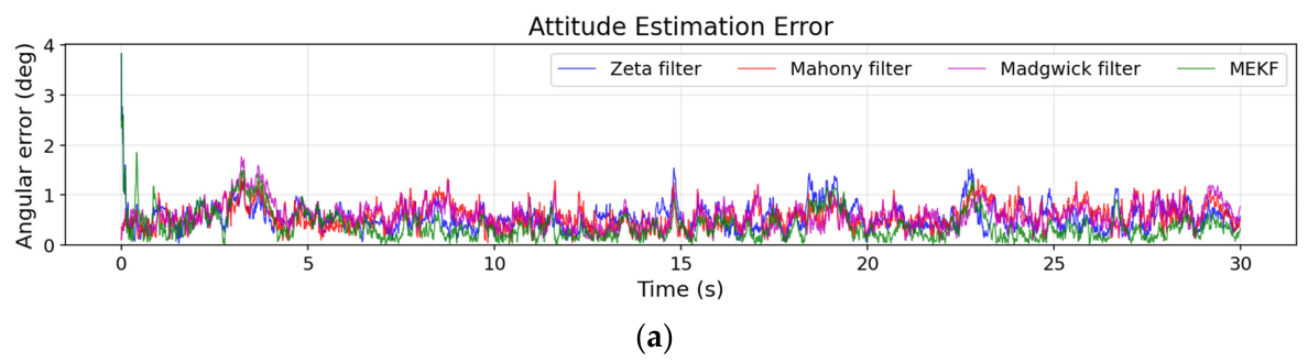
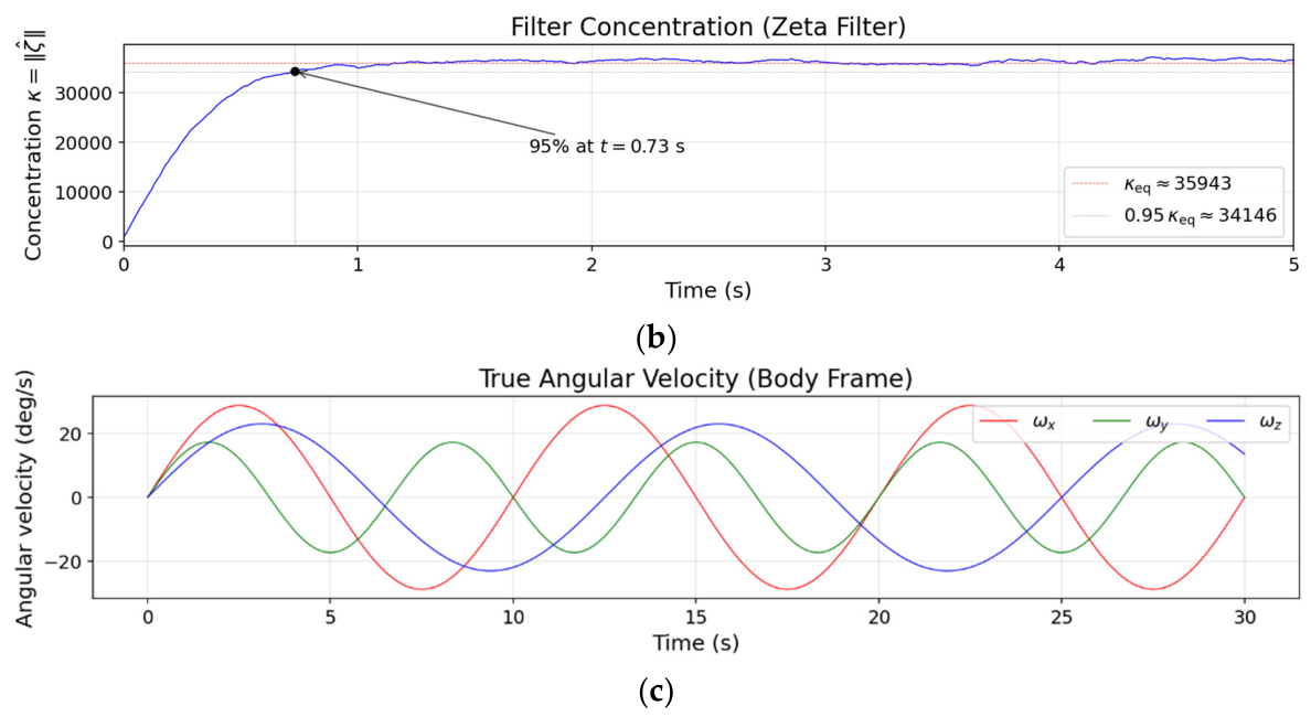
Figure 2 shows the angular estimation error and filter concentration over the simulation. With optimally tuned parameters, all four filters track the dynamic trajectory: MEKF achieves RMSE $0.45°$, Mahony $0.52°$, Madgwick $0.52°$, and the Zeta filter $0.60°$ (after $1 \mathrm{s}$ transient). With the magnetometer weight available for empirical tuning, the complementary filters edge out the Zeta filter under this strongly anisotropic noise—the flip side of the conservative weakest-axis projection (24), which deliberately discards the surplus information of the stronger axes. The Zeta filter in turn, is the only one of the three whose optimum requires no empirical fit (residual scale 0.97). The concentration $\kappa =‖\widehat{\zeta }‖$ rises rapidly from zero (uniform prior) and stabilizes near the predicted equilibrium, confirming the convergence analysis.

3.1.3. Convergence from Wrong Initial Condition

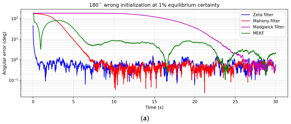
Figure 3 tests global convergence by initializing all four filters at a $180°$ wrong orientation. To provide a fair comparison between filters with internal uncertainty states, the Zeta filter and MEKF are initialized at 1% of their respective equilibrium certainty: ${\kappa }_0=0.01 {\kappa }_{\mathit{eq}}$ for the Zeta filter and $\mathit{tr}\left(P_0\right)=\mathit{tr}\left(P_{\mathit{eq}}\right)/0.01$ for the MEKF. The Mahony and Madgwick filters use fixed gains and do not maintain an internal uncertainty state, so they are initialized with only the wrong quaternion. The Zeta filter converges rapidly: the additive update injects ${\kappa }_{\mathit{obs}}$ in the correct direction, dominating the weak incorrect prior. The MEKF also converges but exhibits transient oscillations due to linearization at large angles. The Mahony and Madgwick filters recover more slowly from the antipodal initial condition.

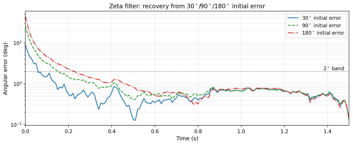
The behavior is consistent across initial error magnitudes: repeating the experiment with 30°, 90°, and 180° initial errors, the Zeta filter re-enters a 2° error band within 0.06, 0.15, and 0.23 s respectively, versus 0.03–6.6 s for Mahony, 1.4–25.4 s for Madgwick, and 0.4–22.5 s for the MEKF (whose linearized update oscillates at large angles). For the Zeta filter, the three recovery transients are shown in Figure 3: on a logarithmic error scale they run parallel, the signature of the uniform per-cycle contraction rate proved in Section 2.5.

This experiment should be read as probing the value of an explicit uncertainty state rather than raw algorithmic superiority: the Zeta filter and the MEKF can declare low confidence in their initial attitude and consequently defer to the measurements, whereas the Mahony and Madgwick filters recover at a rate fixed by the same gains that govern steady-state tracking—a structural property, transparently tied to the initialization choice. What the Zeta filter adds beyond the MEKF’s comparable behavior is the guarantee: the recovery is provably global with a uniform contraction rate (Section 2.5), including the exact antipodal case where linearized and smooth filters offer no such assurance.

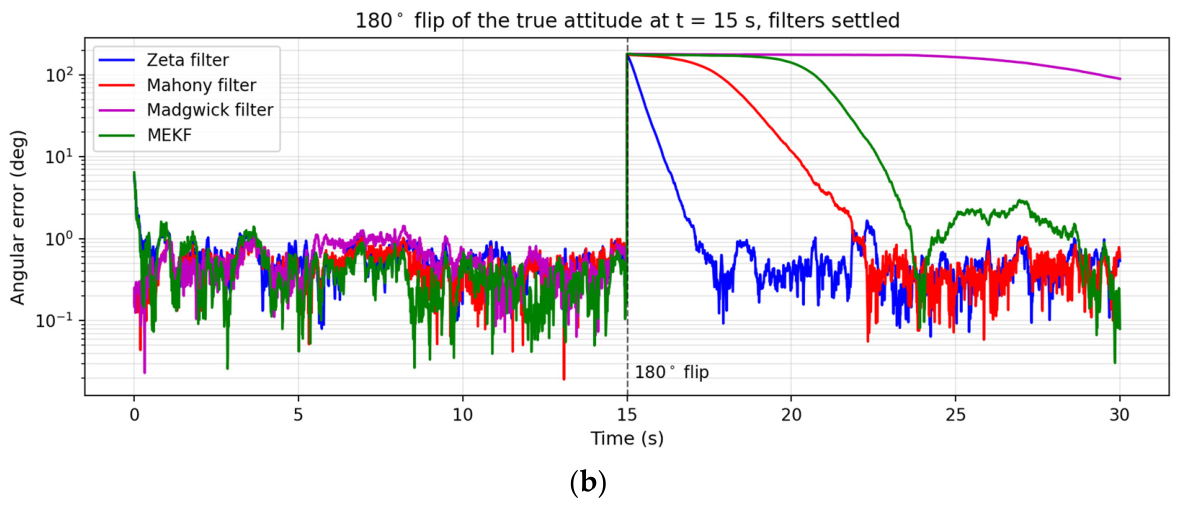
The complementary experiment (Figure 4b) removes the initialization choice from the picture entirely. All four filters first track normally for 15 s and settle at their certainty equilibria; the true attitude is then flipped by 180° in the world frame with no gyroscope transient—the body rates remain valid for the flipped trajectory, so only the vector measurements report the change—leaving every filter confidently wrong by 180°. This is the worst case admitted by the theorem of Section 2.5: the settled concentration sits near the ceiling, so the contraction operates at its slowest rate, ${\rho }_{eq}={\kappa }_{obs}/{\kappa }_{eq}\approx 0.024$. Iterating the exact recursion (32) from the cut locus predicts re-entry into the 2° band after 181 updates (1.81 s); the measured recovery takes 1.76 s, a 3% agreement. The slower transient relative to the (a) panel is the Bayes-correct price of confidence—a filter at equilibrium certainty should resist measurements that contradict it—and the concentration never collapses along the way (it stays within 0.78–1.05 ${\kappa }_{eq}$): by the sign selection every update adds concentration, so the state swings its direction while retaining its certainty. The comparison confirms the structural reading of the top panel: Mahony recovers in 6.7 s, the same rate as from the wrong initialization—fixed gains are blind to confidence—Madgwick does not re-enter the band within the 15 s remaining (consistent with its 25.4 s recovery above), and the MEKF takes 12.4 s, its small steady-state gains admitting the contradicting evidence only gradually.

3.1.4. Noise Sensitivity

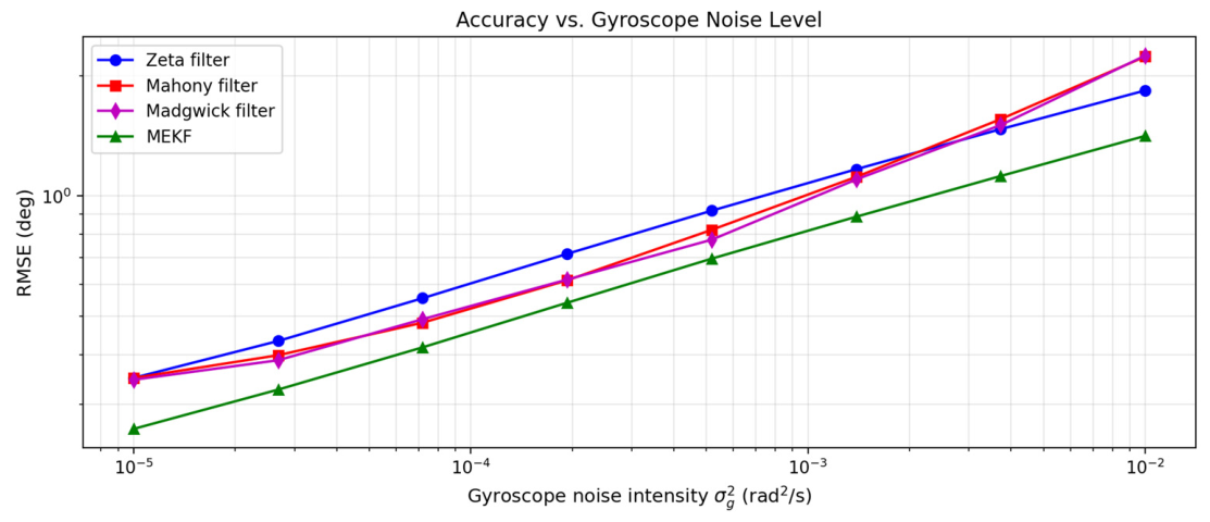
Figure 4 shows RMSE as a function of gyroscope noise intensity ${\sigma }_g^2$ over three orders of magnitude, with all lightweight filters retuned at each noise level and the MEKF using true noise parameters throughout. The MEKF provides the best accuracy at all noise levels. Among the lightweight filters, the empirically tuned Mahony and Madgwick hold an 8–15% margin over the Zeta filter at low and moderate gyroscope noise; the ordering reverses at high gyroscope noise, where the Zeta filter is clearly ahead (1.8° vs. 2.2° at ${\sigma }_g^2={10}^{-2}\mathrm{r}\mathrm{a}{\mathrm{d}}^2/\mathrm{s}$). The Zeta filter’s theoretical weight (24) serves unretuned across the entire sweep: at every noise level the grid-searched optimal scale stays near the fixed theoretical value of unity (0.93–1.43 over both sweeps). All four degrade gracefully as noise increases.

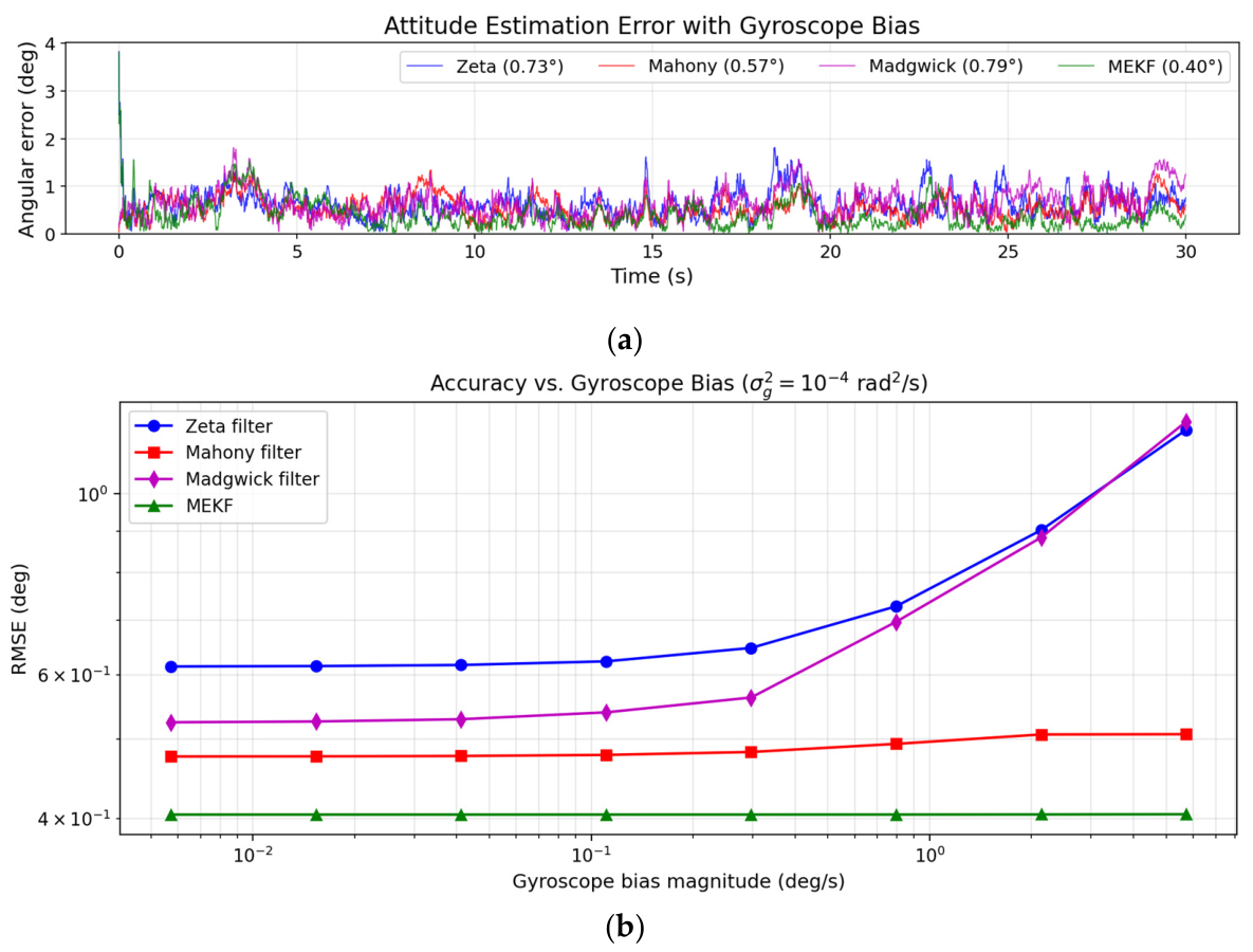
3.1.5. Bias Robustness

Figure 5 evaluates performance with a constant gyroscope bias of ~0.5°/s per axis. All filters are retuned for this scenario; notably, the Mahony filter’s integral gain $k_i$ is now optimized alongside $k_p$, enabling online bias estimation. RMSE is computed after a $15 \mathrm{s}$ transient to allow bias estimators to converge. The MEKF handles bias naturally through its 6-state error model (RMSE $0.41°$). The Mahony filter, with $k_i>0$, estimates bias and achieves $0.49°$—outperforming the Zeta filter ($0.73°$) and Madgwick ($0.70°$), neither of which models bias. As expected, filters without bias estimation (Zeta, Madgwick) degrade with increasing bias, while the Mahony integral term and MEKF bias state sustain accuracy.

Without a bias state, the Zeta filter’s error nevertheless remains bounded: each cycle, the bias-induced drift $1/2‖b‖\Delta t$ is balanced by the update contraction factor $1/\left(1+\rho \right)$ of Section 2.5, and the error settles on a stationary, bias-dependent floor

$${\tilde{\Theta }}_{floor}\approx ‖b‖\sqrt{{\displaystyle \frac{\Delta t}{\alpha {\sigma }_g^2{\kappa }_{obs}}}}$$

(37)

Runs of 120 s at the fixed theoretical weight, over biases of 0.1–5°/s, confirm both the stationarity (RMSE over disjoint late windows agrees at every bias level) and the linear law (correlation 0.9997, fitted proportionality constant 0.95 against the theoretical value of unity); for the baseline configuration the floor crosses 1° at $‖b‖\approx 2.6°/\mathrm{s}$, several times the post-calibration turn-on bias of consumer MEMS gyroscopes. In the sweep of Figure 6, the Zeta curve rises more slowly than (37) because the per-level retuning raises the measurement weight against large biases. Sustained operation with larger uncompensated biases favors filters with explicit bias estimation.

3.1.6. Isotropic Observation Noise

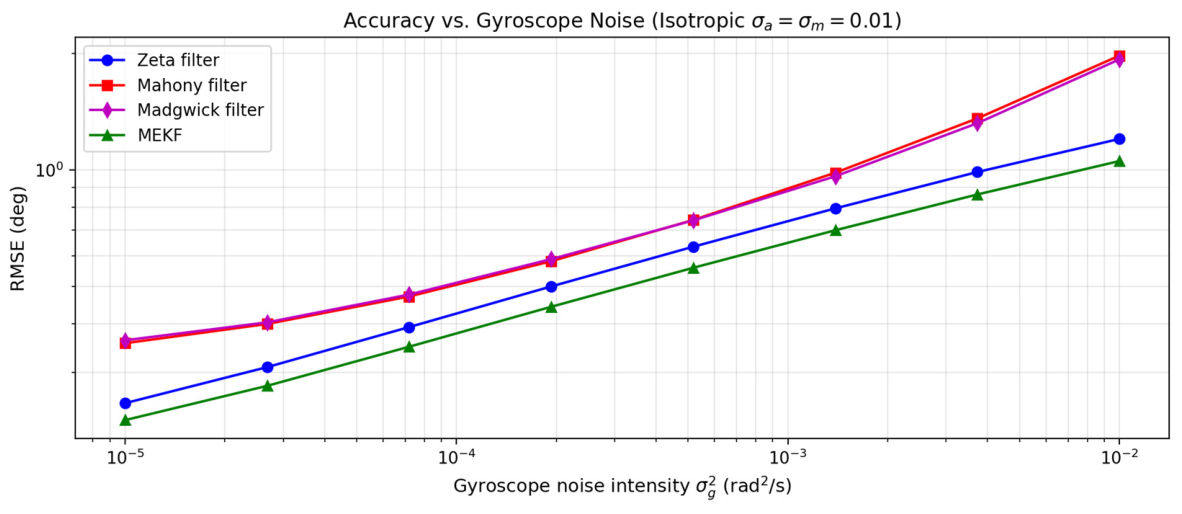
The preceding results use anisotropic observation noise (${\sigma }_a=0.002$, ${\sigma }_m=0.03$), reflecting typical MEMS accelerometer–magnetometer pairs. However, the vMF measurement model assumes isotropic noise on $S^3$. To evaluate the filter where this assumption holds exactly, the noise sweep is repeated with equal observation noise ${\sigma }_a={\sigma }_m=0.01$, modeling situations where measurement noise is comparatively isotropic.

Table 2 summarizes the tuning parameters and RMSE under isotropic noise at the baseline gyroscope noise level. The Zeta filter achieves the lowest RMSE among the lightweight filters, closing the gap with the MEKF; notably, the Mahony optimum reverts to the classical equal weighting ($w_m$ = 0.5), so the second tuning parameter buys the complementary filters nothing once the noise is isotropic.

Figure 7 shows RMSE vs. gyroscope noise intensity under isotropic observation noise. The Zeta filter attains the lowest lightweight RMSE at every noise level—by ~15% at the baseline, widening to ~40% at the highest gyroscope noise—and stays within ~15% of the MEKF across the entire range. The vMF natural parameter update is inherently non-linear and exact for isotropic spherical noise, achieving in a single vector addition what the MEKF approximates through linearized Kalman updates, with no covariance propagation, matrix inversion, or linearization involved.

3.1.7. Validation on Recorded Flight Data

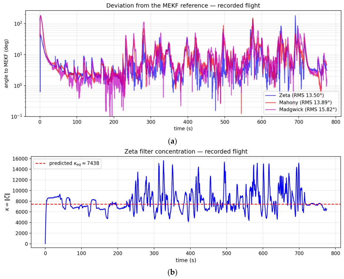
To complement the synthetic experiments, the four filters were run on a recorded flight of a small tailless flying-wing UAV (2 m span, ≈1.2 kg maximum take-off mass, electric tractor propeller), logged with its onboard PRP-W2 flight-parameter recorder [29]: 13 min of gyroscope, accelerometer, and magnetometer data at 100 Hz, with 10 Hz GPS. The logger timebase was established from the GPS UTC channel, and the magnetometer was hard-iron calibrated by a sphere fit over in-flight samples—the fitted field magnitude (50.3 µT) and inclination (65°) match the reference geomagnetic values for the flight location. Sensor noise levels estimated from the data (${\sigma }_g^2$ = 6.7 × 10⁻⁵ rad²/s, ${\sigma }_a$ = 0.096, ${\sigma }_m$ = 0.017) show an anisotropy reversed relative to the simulation baseline: on this vehicle the propeller-induced vibration makes the accelerometer, not the magnetometer, the noisy channel—consistent with the strong propulsion-induced IMU vibration reported for this airframe [29]—which (24) absorbs without any change to the filter.

In this test the MEKF—with a gyro-bias state and the estimated noise parameters—serves as the reference estimator: each lightweight filter’s single parameter is calibrated for best agreement with it on a decimated stream, and the full-rate deviation is evaluated (absolute accuracy is assessed against an independent reference in Section 3.1.8). Over the flight, the Zeta filter tracks the reference most closely of the three lightweight filters (

Table 3. UAV flight: RMS deviation of each lightweight filter from the MEKF reference estimator (not a ground truth) over the 13 min flight.

Filter	Full Attitude	Tilt Only
Zeta	$13.5°$	$5.7°$
Mahony	$13.9°$	$7.9°$
Madgwick	$15.8°$	$6.6°$

). The deviations of all three are heading-dominated and concentrate in the sustained coordinated turns that make up most of this flight, where the specific force ceases to indicate gravity and unaided MARG attitude is intrinsically ambiguous; these figures therefore characterize the scenario more than they rank the filters. The sharpest quantitative outcome concerns the concentration dynamics: the equilibrium predicted from the estimated noise parameters, ${\kappa }_{eq}$ ≈ 7400, matches the observed median concentration over the flight to within 1% (Figure 8), validating the prediction model of Section 2.3 and Section 2.5 on real sensor data.

3.1.8. Evaluation Against an EFIS Attitude Reference

The second flight experiment evaluates absolute accuracy against an independent reference: a 42 min flight of an MP-02A “Czajka” light aircraft whose panel-mounted Dynon SkyView D-700 electronic flight instrument system (EFIS) logged its certified-grade attitude solution (roll, pitch, heading; reference accuracy ±1° roll/pitch static and ±2.5° dynamic, per ETSO-C201) at 8 Hz, while an Apple iPhone 13 rigidly mounted in the cockpit recorded raw gyroscope, accelerometer, and magnetometer streams via MATLAB Mobile (v9.12) at 16.7 Hz; the flight and sensor logs are those of [30]. The two logs were synchronized by correlating GPS ground speed (correlation coefficient 0.99); the unknown phone-to-aircraft mounting rotation was estimated by a gravity-direction Wahba fit, and the magnetometer was ellipsoid-calibrated on in-flight samples. Consumer MEMS sensors at 16.7 Hz in a vibrating cockpit constitute a deliberately harsh but realistic low-cost scenario.

To prevent the tuned parameters from being fitted to the very data on which accuracy is reported, the flight is split into halves: each filter’s free parameters are selected on the first half only, and all results are reported on the second half, at the reference instants of the airborne portion (GPS ground speed above 8 m/s). Each filter receives the same two-dimensional tuning freedom, spanning its natural parameter space—for Mahony and Madgwick the feedback gain and the magnetometer weight, for the MEKF the two measurement noise scales, and for the Zeta filter the two observation noise scales (${\sigma }_a$, ${\sigma }_m$) with the theoretical ${\kappa }_{obs}$ of (24) used unchanged.

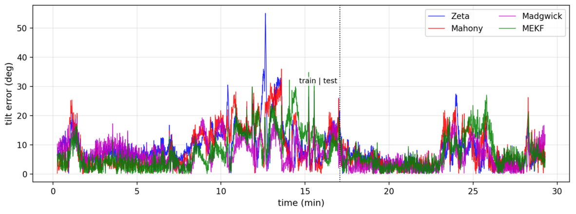
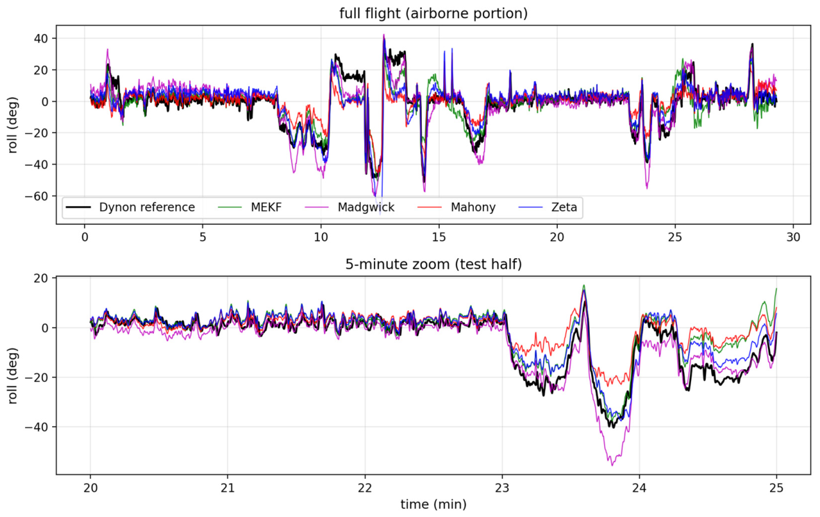
On the test half, the tilt error against the reference—the angle between estimated and reference gravity directions, insensitive to the heading datum—is summarized in

Table 4. EFIS-referenced flight, test half (airborne, GPS ground speed above $8 \mathrm{m}/\mathrm{s}$): tilt error against the Dynon reference and datum-free heading-rate error.

Filter	Tilt RMSE	Tilt Median	Heading Rate
Madgwick	$6.5°$	$3.8°$	$1.1°/\mathrm{s}$
Zeta	$6.8°$	$4.7°$	$2.1°/\mathrm{s}$
Mahony	$7.5°$	$4.4°$	$1.4°/\mathrm{s}$
MEKF	$8.0°$	$4.9°$	$2.1°/\mathrm{s}$

(Figure 9 and Figure 10); restricting the evaluation to strictly airborne samples by barometric altitude raises all four errors by 1–2° without changing the ordering. Three observations qualify these numbers. First, the four filters land within 1.5° of one another—differences comparable to the selection noise of the protocol: under real flight disturbances that are systematic rather than white (sustained coordinated-turn accelerations, cockpit magnetic interference), every filter’s winning configuration corresponds to heavy measurement distrust, and no algorithm can recover information that the measurements do not carry. Second, the MEKF illustrates the cost of optimality assumptions: configurations that trust the magnetometer according to its apparent (white) noise level are catastrophic here (14–33° RMSE) because the joint update couples the systematically disturbed magnetometer into the tilt estimate; it becomes competitive only with its measurement model nearly disabled, at 13× the computational cost of the Zeta filter. Third, the Zeta filter’s winning configuration keeps the theoretical measurement weight (24) unchanged—consistent with the parameter-free behavior established in the simulations—with only its two observation-noise scales fitted (${\sigma }_a$ = 0.40, ${\sigma }_m$ = 0.07, inflated far above the sensors’ bench noise and absorbing the in-flight disturbance level), whereas the Mahony/Madgwick/MEKF winners are pure empirical fits. Absolute heading is not evaluable in this cockpit (the calibrated field magnitude is 29 µT against the ~50 µT geomagnetic reference, and the phone-mounted magnetometer datum wanders with respect to the aircraft); Table 4 therefore reports the datum-free heading-rate error instead. Finally, the concentration dynamics receive the same confirmation as on the first flight: at this 16.7 Hz update rate, the equilibrium predicted from the estimated sensor noise, ${\kappa }_{eq}$ ≈ 5400, matches the median concentration the filter actually reached to within 1%.

3.1.9. Computational Cost

Table 5. Computational cost per predict–update cycle (two reference vectors). The Zeta filter count includes QUEST measurement construction.

Filter	Add/Sub	Mul	Div	Sqrt/Trig	Total
Mahony	98	119	10	3	230
Zeta	158	209	32	12	411
Madgwick	223	240	14	5	482
MEKF	2607	2734	102	12	5455

lists the measured per-cycle cost of the four filters: reference C implementations, verified against the simulation code at machine precision over the full 30 s stream, were instrumented at the arithmetic-operator level and run over the recorded reference stream, so every executed addition, multiplication, division, square root, and trigonometric call is counted.

None of the four implementations is performance-optimized, and all are written in the same plain style—reference-equation structure, generic vector and matrix helpers, no hand-shared subexpressions—so the ratios between rows, rather than the absolute counts, are the meaningful quantity. For the Madgwick filter, whose authors distribute a hand-optimized reference implementation [10], both forms were implemented and verified equivalent to machine precision; the table reports the style-matched plain form, and the hand-optimized original—358 operations against 482—is discussed with the on-target results below.

The Zeta filter’s own predict–update core is small (one quaternion multiplication, the rational decay, one dot product, a sign check, and a vector addition—under 60 operations); the bulk of its 411-operation total is the QUEST solve (attitude profile matrix, characteristic quartic by Newton–Raphson, optimal-quaternion extraction), with the closed-form evaluation (25) of ${\kappa }_{obs}$ adding only ~15 operations. It thus costs about 1.8× the Mahony filter and 0.85× the Madgwick filter—the same lightweight class, with no matrix larger than 3 × 3 and no decomposition or inversion.

The MEKF, in a straightforward dense implementation, measures 5455 operations: the covariance propagation ΦPΦ^T + Q, the gain computation with a 6 × 6 innovation inversion, and the Joseph-form update each contribute several 6 × 6 matrix products (432 multiply—adds apiece). Exploiting the sparsity of the measurement Jacobian and the symmetry of P would reduce the constant severalfold, but not the class: the measured cost is 13.3× the Zeta filter, and the MEKF additionally carries 6 × 6 = 36 covariance state variables, whereas the Zeta filter’s complete state is a single four-vector. Wall-clock measurements on a desktop CPU show the same ordering (MEKF ~10× the Zeta filter per cycle).

The ordering also holds on representative embedded hardware (

Table 6. Measured on-target cost per predict–update cycle: STM32F429 (Cortex-M4F, 180 MHz), single precision FPU (Floating-Point Unit), captured via DWT (Data Watchdog and Trace) cycle counter, averaged over the reference stream.

Filter	Cycles	Time μs	×Zeta
Mahony	986	5.5	0.30
Madgwick	3014	16.7	0.92
Zeta	3 265	18.1	1.00
MEKF	41 741	231.9	12.8

): compiled in single precision—the native width of the target’s hardware floating-point unit (FPU)—for an STM32F429 microcontroller (Cortex-M4F, 180 MHz) and measured on-target with the DWT (Data Watchpoint and Trace) cycle counter over the reference stream, every filter sits far inside the 10 ms budget of a 100 Hz loop. The hand-optimized original Madgwick implementation, measured alongside, completes the picture: it executes its 358 operations in 976 cycles (5.4 µs), 3.1× faster than its mathematically identical plain-style form—straight-line code holds intermediates in FPU registers, whereas the helper-structured implementations pay load/store traffic that operation counts do not record. Implementation style thus moves the constant severalfold within the lightweight class, and comparable hand-tuning is available to every row of the table. The instrumented benchmark and verification harness are published together with the simulation code.

4. Conclusions

This article has presented an attitude filter whose sole state is the vMF natural parameter $\widehat{\zeta }=\kappa \mu \in {\mathbb{R}}^4$, with additive measurement updates, a continuous-time prediction ODE grounded in the high-$\kappa$ asymptote of exact vMF concentration dynamics [17], QUEST-based measurement construction [19] with a Fisher-curvature-matched measurement concentration, antipodal switching for the quaternion double cover, and a global convergence analysis: the concentration is confined to an attracting band, and the attitude error contracts exponentially from every initial condition, including the antipodal one. The filter operates entirely in unconstrained ${\mathbb{R}}^4$ without normalization constraints, linearization, or covariance matrix propagation, and its construction is left-invariant under rotations of the reference frame.

In the scenarios evaluated, the filter approaches the accuracy of the MEKF—within roughly 13% under isotropic observation noise and 33% at the anisotropic baseline—while dispensing with the $6\times 6$ covariance propagation and matrix inversion that the MEKF requires at each update step. Against lightweight filters of similar computational cost (Mahony, Madgwick), the outcome depends on the noise structure: under the strongly anisotropic noise typical of accelerometer–magnetometer pairs, the complementary filters equipped with an empirically tuned magnetometer weight attain ~10% lower error—the price of the conservative weakest-axis projection (24)—while under isotropic observation noise, and at high gyroscope noise in either regime, the Zeta filter attains the lowest lightweight error, with the vMF measurement model exact in the isotropic-noise regime. It additionally offers structural benefits: a built-in uncertainty measure ($\kappa =\Vert \widehat{\zeta }$), zero-state initialization, a theoretically grounded measurement weight requiring no per-scenario tuning, and the global convergence guarantee, none of which Mahony or Madgwick offer. On recorded flight data, where systematic disturbances dominate, and all four filters perform within the selection noise of the evaluation protocol, the Zeta filter is distinguished not by margin but by needing no empirical reweighting: its winning configuration uses the theoretical measurement weight unchanged.

The present formulation has four principal limitations. First, the scalar concentration can carry only isotropic attitude information: the anisotropic (Bingham-type) information delivered by real sensor pairs is projected onto its weakest-axis reduction in (24); under strongly anisotropic noise this concedes a modest accuracy margin (~10%) to complementary filters given an empirically tuned magnetometer weight, and the Zeta filter’s accuracy advantage is realized when the observation noise is near-isotropic. Second, there is no gyroscope bias state, so accuracy degrades with uncompensated bias (Section 3.1.5). Third, the measurement construction assumes two simultaneously sampled vector observations; single-vector updates, such as accelerometer-only phases, require an extension of the ${\kappa }_{obs}$ construction to rank-deficient $F$. Fourth, the real-flight evidence has bounded resolution: the UAV flight of Section 3.1.7 lacks an on-board attitude reference (it validates consistency and the concentration dynamics), and in the EFIS-referenced evaluation the systematic in-flight disturbances dominate the error budget, so all four filters perform within the selection noise of the protocol and the comparison cannot resolve accuracy margins between them under real flight conditions—it establishes membership in the achievable class, physically interpretable tuning, and the validity of the theoretical measurement weight, not superiority.

The current formulation does not include gyroscope bias estimation; extending the state to include it is future work. Further direction of research should also include improvement to the treatment of the sensor’s measurement error anisotropy; decoupling the observation vectors by formulating a dual vMF filter on $S^2$ could be a promising approach. The filter analysis would also benefit from the systematic comparison against sampling-based Bayesian filters (particle and unscented variants) under non-Gaussian noise.

References

1. Lu, Y.; Li, Z.; Xiong, J.; Lv, K. Adaptive UAV Navigation Method Based on AHRS. Sensors 2024, 24, 2518. [Google Scholar] [CrossRef] [Scilit] [PubMed]
2. Yu, C.; Wang, P.; Han, S.; Bai, S. Research on Navigation Technology of Small UAV Based on MEMS Sensor. In Proceedings of the 2022 International Conference on Intelligent Manufacturing, Advanced Sensing and Big Data (IMASBD), Guilin, China, 15–17 October 2022; pp. 57–63. [Google Scholar] [CrossRef] [Scilit]
3. Yang, Y.; Liu, X.; Zhang, W.; Liu, X.; Guo, Y. A Nonlinear Double Model for Multisensor-Integrated Navigation Using the Federated EKF Algorithm for Small UAVs. Sensors 2020, 20, 2974. [Google Scholar] [CrossRef] [Scilit] [PubMed]
4. Ko, N.Y.; Youn, W.; Choi, I.H.; Song, G.; Kim, T.S. Features of Invariant Extended Kalman Filter Applied to Unmanned Aerial Vehicle Navigation. Sensors 2018, 18, 2855. [Google Scholar] [CrossRef] [Scilit] [PubMed]
5. Guardeño, R.; López, M.J.; Sánchez, V.M. MIMO PID Controller Tuning Method for Quadrotor Based on LQR/LQG Theory. Robotics 2019, 8, 36. [Google Scholar] [CrossRef] [Scilit]
6. Chen, C.-L.; He, R.; Peng, C.-C. Development of an Online Adaptive Parameter Tuning vSLAM Algorithm for UAVs in GPS-Denied Environments. Sensors 2022, 22, 8067. [Google Scholar] [CrossRef] [Scilit] [PubMed]
7. Weber, C.; Eggert, M.; Udelhoven, T. Flight Attitude Estimation with Radar for Remote Sensing Applications. Sensors 2024, 24, 4905. [Google Scholar] [CrossRef] [Scilit] [PubMed]
8. Citroni, R.; Di Paolo, F.; Livreri, P. A Novel Energy Harvester for Powering Small UAVs: Performance Analysis, Model Validation and Flight Results. Sensors 2019, 19, 1771. [Google Scholar] [CrossRef] [Scilit] [PubMed]
9. Mahony, R.; Hamel, T.; Pflimlin, J.-M. Nonlinear complementary filters on the special orthogonal group. IEEE Trans. Autom. Control 2008, 53, 1203–1218. [Google Scholar] [CrossRef] [Scilit]
10. Madgwick, S.O.H.; Harrison, A.J.L.; Vaidyanathan, R. Estimation of IMU and MARG orientation using a gradient descent algorithm. In Proceedings of the IEEE International Conference on Rehabilitation Robotics (ICORR), Zurich, Switzerland, 29 June–1 July 2011; pp. 1–7. [Google Scholar] [CrossRef] [Scilit] [PubMed]
11. Majewski, K.; Żugaj, M. Adaptive Kalman Filter for UAV Dynamic Flight Maneuvers. In Proceedings of the Research and Education in Aircraft Design (READ) Conference 2024, Warsaw, Poland, 6–8 November 2024. [Google Scholar]
12. Munguía, R.; Urzua, S.; Grau, A. EKF-Based Parameter Identification of Multi-Rotor Unmanned Aerial VehiclesModels. Sensors 2019, 19, 4174. [Google Scholar] [CrossRef] [Scilit] [PubMed]
13. Kada, B.; Munawar, K.; Shaikh, M.S.; Hussaini, M.A.; Al-Saggaf, U.M. UAV Attitude Estimation Using Nonlinear Filtering and Low-Cost MEMS Sensors. IFAC-PapersOnLine 2016, 49, 521–528. [Google Scholar] [CrossRef] [Scilit]
14. Lee, T. Bayesian attitude estimation with the matrix Fisher distribution on SO3. IEEE Trans. Autom. Control 2018, 63, 3377–3392. [Google Scholar] [CrossRef] [Scilit]
15. Kurz, G.; Gilitschenski, I.; Hanebeck, U.D. Unscented von Mises–Fisher filtering. IEEE Signal Process. Lett. 2016, 23, 463–467. [Google Scholar] [CrossRef] [Scilit]
16. Glover, J.; Kaelbling, L.P. Tracking 3-D Rotations with the Quaternion Bingham Filter; Technical Report MIT-CSAIL-TR-2013-005; MIT Computer Science and Artificial Intelligence Laboratory: Cambridge, MA, USA, 2013; Available online: https://dspace.mit.edu/handle/1721.1/78248 (accessed on 17 May 2026).
17. Tronarp, F.; Hostettler, R.; Särkkä, S. Continuous-discrete von Mises–Fisher filtering on S2 for reference vector tracking. In Proceedings of the 21st International Conference on Information Fusion (FUSION), Cambridge, UK, 10–13 July 2018; pp. 1345–1352. [Google Scholar] [CrossRef] [Scilit]
18. Hornik, K.; Grün, B. On conjugate families and Jeffreys priors for von Mises–Fisher distributions. J. Stat. Plan. Inference 2013, 143, 992–999. [Google Scholar] [CrossRef] [Scilit] [PubMed]
19. Shuster, M.D.; Oh, S.D. Three-axis attitude determination from vector observations. J. Guid. Control Dyn. 1981, 4, 70–77. [Google Scholar] [CrossRef] [Scilit] [PubMed]
20. Wahba, G. Problem 65-1: A least squares estimate of satellite attitude. SIAM Rev. 1965, 7, 409. [Google Scholar] [CrossRef] [Scilit]
21. Markley, F.L.; Crassidis, J.L. Fundamentals of Spacecraft Attitude Determination and Control; Space Technology Library; Springer: New York, NY, USA, 2014; Volume 33, Correction in Fundamentals of Spacecraft Attitude Determination and Control; Space Technology Library; Springer: New York, NY, USA, 2019; Volume 33. https://doi.org/10.1007/978-1-4939-0802-8_13. [Google Scholar]
22. Shuster, M.D. Maximum likelihood estimation of spacecraft attitude. J. Astronaut. Sci. 1989, 37, 79–88. [Google Scholar]
23. Minka, T.P. Expectation propagation for approximate Bayesian inference. In Proceedings of the 17th Conference on Uncertainty in Artificial Intelligence (UAI), Seattle, WA, USA, 2–5 August 2001; pp. 362–369. [Google Scholar]
24. Barrau, A.; Bonnabel, S. The invariant extended Kalman filter as a stable observer. IEEE Trans. Autom. Control 2017, 62, 1797–1812. [Google Scholar] [CrossRef] [Scilit]
25. Khalil, H.K. Nonlinear Systems, 3rd ed.; Prentice Hall: Upper Saddle River, NJ, USA, 2002; ISBN 978-0130673893. [Google Scholar]
26. Solà, J. Quaternion kinematics for the error-state Kalman filter. arXiv 2017, arXiv:1711.02508. [Google Scholar] [CrossRef] [Scilit]
27. Trumpf, J.; Mahony, R.; Hamel, T.; Lageman, C. Analysis of non-linear attitude observers for time-varying reference measurements. IEEE Trans. Autom. Control 2012, 57, 2789–2800. [Google Scholar] [CrossRef] [Scilit]
28. Bhat, S.P.; Bernstein, D.S. A topological obstruction to continuous global stabilization of rotational motion and the unwinding phenomenon. Syst. Control Lett. 2000, 39, 63–70. [Google Scholar] [CrossRef] [Scilit]
29. Zięba, W.; Rzucidło, P.; Wałek, Ł. Design and Flight Tests of a Small Flying Wing UAV. Aerospace 2026, 13, 240. [Google Scholar] [CrossRef] [Scilit]
30. Kaczyński, J.; Rzucidło, P. A Concept for Smartphone-Based Emergency Flight Data Indication Systems in Light Aircraft. Sensors 2026, 26, 3368. [Google Scholar] [CrossRef] [Scilit] [PubMed]
Figure 1. Validation of the asymptotic approximation A p / A p 2 p 1 κ 2 on S 3 ( p = 4 ). (a): relative approximation error <1% for κ >   100 ; (b): exact Bessel ratio (blue) vs. asymptotic 2 3 κ 2 (red dashed).
Inventions 11 00076 g001
Figure 2. Tracking performance comparison. (a): angular error for the Zeta filter (blue), Mahony (red), Madgwick (magenta), and MEKF (green); (b): concentration κ = ζ ^ of the Zeta filter, featuring theoretical equilibrium κ eq (red dashed) and 95% settling threshold (black dotted); (c): true body-frame angular velocity.
Inventions 11 00076 g002aInventions 11 00076 g002b
Figure 3. Zeta filter recovery from 30, 90 and 180 initial attitude errors (first 1.5 s, logarithmic scale). The parallel slopes reflect the uniform per-cycle contraction rate of Section 2.5, independent of the initial error.
Inventions 11 00076 g003
Figure 4. Global convergence experiments for the Zeta filter (blue), Mahony (red), Madgwick (magenta), and MEKF (green); logarithmic error scale. (a) 180° wrong initial condition, Zeta filter and MEKF at 1% of equilibrium certainty. (b) 180° world-frame flip of the true attitude at t = 15   s with all filters settled at equilibrium certainty and no gyroscope transient.
Inventions 11 00076 g004aInventions 11 00076 g004b
Figure 5. RMSE vs. gyroscope noise intensity for the Zeta filter (blue), Mahony (red), Madgwick (magenta), and MEKF (green). All filters are at their optimal tuning at each noise level.
Inventions 11 00076 g005
Figure 6. Bias robustness. (a): attitude estimation error with a constant gyroscope bias of ~0.5°/s (RMSE values shown in legend). (b): RMSE vs. gyroscope-bias magnitude. Filters with bias estimation (MEKF, Mahony) remain flat; the Zeta and Madgwick filters, which do not model bias, degrade as bias grows.
Inventions 11 00076 g006
Figure 7. RMSE vs. gyroscope noise intensity with isotropic observation noise ( σ a = σ m = 0.01 ) for the Zeta filter (blue), Mahony (red), Madgwick (magenta), and MEKF (green). All filters are at their optimal tuning at each noise level.
Inventions 11 00076 g007
Figure 8. Recorded flight evaluation. (a): deviation of the lightweight filters from the MEKF reference (logarithmic scale), (b): Zeta filter concentration κ = ζ ^ (blue) against the equilibrium predicted from the estimated sensor noise (red dashed).
Inventions 11 00076 g008
Figure 9. EFIS-referenced flight evaluation: aircraft roll angle from the four filters (phone sensors, mounting rotation estimated on the training half) against the Dynon reference.
Inventions 11 00076 g009
Figure 10. EFIS-referenced flight evaluation: tilt error of each filter against the Dynon reference, with the train/test split marked.
Inventions 11 00076 g010