1. Introduction
With the continuous increase in the installed capacity of renewable energy such as wind power and photovoltaic (PV) power, the proportion of renewable energy output in load demand has gradually increased, leading to an increasing demand for flexibility in the operation of power systems to maintain power balance [
1].
As an auxiliary indicator associated with flexibility demand, complementary characteristics reflect the source of flexibility demand from another perspective. In existing studies on complementarity, numerous scholars have researched the complementary characteristics between wind power and PV power themselves, as well as different combinations with hydropower [
2]. The main goal of these studies is to maintain the stability of the total output of various renewable energy combinations, and complementarity is defined based on this. Essentially, it utilizes the reduction effect on the coefficient of variation caused by the different output change trends of various types of renewable energy or the same type of renewable energy in different regions due to varying meteorological conditions [
3,
4]. Research in [
5] shows that wind–solar complementarity can reduce volatility by 34.4%; ref. [
6] defines the real-time complementarity rate using the weighted ratio of the modulus of the fluctuation values of individual and combined wind and PV outputs and describes the complementarity of wind and PV outputs by the mean value of the real-time complementarity rate. However, due to the introduction of weighted values, this indicator may exceed 1 when the fluctuations of wind and PV outputs are in the same direction, resulting in loss of accuracy.
Among flexibility resources, traditional supporting power sources such as nuclear power and thermal power mainly bear the base load. They have slow ramping rates, and their physical characteristics do not support high-frequency and large-amplitude regulation, so their output is expected to be smooth and stable. Among resources with good flexibility, hydropower and pumped storage are highly dependent on geographical conditions and cannot be constructed on a large scale in most regions; gas-fired power generation has a fast regulation rate but high cost; electrochemical energy storage is not a power source and is prone to problems such as high electricity cost due to low dispatch utilization rate. From the perspective of reducing the demand for flexibility resource regulation during the dispatch of high-proportion new energy power systems, the consistency between renewable energy output and load demand changes provides a better guiding direction for complementarity analysis. Taking load change as the reference value, complementarity is defined as the degree of consistency between renewable energy output and load change based on the source-load matching idea.
Existing studies have primarily quantified the degree of source-sink matching by quantifying differences in statistical correlations or trends. Ref. [
7] defines the “load tracking degree” using the normalized value of the product of deviations and the product of standard deviations between load and bundled power sources within the evaluation period T; refs. [
8,
9] define the “load tracking coefficient” as the average modulus of the difference between the change rate of power generation on the source side and the change rate of load power consumption. Unlike the load tracking degree, which is better when approaching 1, the load tracking coefficient has the same meaning when approaching 0. Both use the concept of average value and are suitable for matching evaluation over a long evaluation period. Ref. [
10] selects the probability that the total renewable energy output is within a certain range above and below the load as the quantitative value of the “load matching degree” indicator. These methods require the support of large-sample data to obtain relatively reliable results and are suitable for retrospective analysis of historical data.
On the other hand, subsequent research has focused on developing more comprehensive or normalized evaluation metrics; yet, challenges persist in parameter setting and intuitiveness. Ref. [
11] weights the standard deviation of the total output of the wind–solar–hydro hybrid energy system, the slope angle of the total output curve at each moment, and the standard deviation of the net load to construct the “source-load difference index” to describe the tracking degree of the total output of the hybrid system to the load. However, it is not normalized, making it difficult to intuitively evaluate the source-load matching degree. On the basis of [
6], ref. [
12] measures the source-load complementarity using the normalized mean value of net load fluctuation; ref. [
13] adjusts the new energy output to the same quantity interval by constructing a matching load proportional to the actual load and evaluates the source-load consistency using the normalized coefficient of the modulus of the difference between source and load change rates. However, how to select the value of its regulation coefficient parameter is not clear. For the purpose of defining this parameter, its value is a random variable affected by installed capacity and climate conditions, making it very difficult to select; in contrast, ref. [
14] describes consistency using the difference between the respective percentage changes of source and load, but ignores the impact of inconsistent base sizes of source and load.
In terms of complementarity calculation methods, in addition to the aforementioned first-order difference, standard deviation, expectation, and other indicators and their combinations, some scholars also use correlation coefficients to evaluate complementarity, such as the Pearson linear correlation coefficient [
5,
14,
15], Spearman rank correlation coefficient [
10,
15,
16], Kendall rank correlation coefficient [
1,
17], etc. However, their evaluation periods are all above the hourly or daily level, lacking applicability to short time scales. At the same time, the above studies all use original measurement data for calculation. With the continuous improvement of sampling rate and accuracy, high-frequency small-amplitude noise in the data has a great impact on the accuracy of the evaluation results based on rank correlation coefficients.
In terms of regulation capacity evaluation, ref. [
18] conducts statistical analysis using indicators such as the probability of insufficient regulation capacity within the evaluation period, which has no real-time guiding significance; ref. [
19] uses sample expansion and kernel density estimation methods to obtain the distribution models of new energy output and load demand respectively and then evaluates the ramping capacity and regulation depth using net load fluctuation values, but does not consider the distribution change of fluctuation values after estimating the distribution; ref. [
20] constructs the distribution function of regulation capacity using a two-state probability model and quantifies the probability and expectation of insufficient regulation capacity according to the distribution function, but lacks a characterization method for forced outage probability.
To address the limitations in existing studies on quantifying source-load complementarity and regulation capability—such as reliance on static or single-dimensional indicators, neglect of temporal consistency and tail dependence structures, sensitivity to data noise, and insufficient integration of fluctuation ranges with credible regulation capacities for dynamic scheduling guidance—this paper proposes a multi-level integrated evaluation framework. First, from the perspective of source-load matching, a complementarity evaluation method is proposed that considers real-time change rates, temporal consistency, and tail dependence. This method combines Improved Complete Ensemble Empirical Mode Decomposition with Adaptive Noise (ICEEMDAN) and a Copula mixture model, thereby more accurately characterizing the dynamic interdependence between sources and loads. Second, the Minkowski sum is introduced to construct the net load fluctuation range, overcoming the limitations of traditional interval methods in capturing extreme fluctuations and coupled relationships. Furthermore, by integrating the Analytic Hierarchy Process (AHP) with probabilistic convolution, a comparative quantification between the fluctuation range and the credible capacity of regulation resources at different evaluation levels is achieved, providing hierarchical decision support for scheduling arrangements. Compared to existing studies, the proposed approach not only emphasizes the synergistic benefits of methodological integration—where ICEEMDAN enhances the decomposition of non-stationary sequences, the Copula mixture model improves the characterization of multi-dimensional and tail dependencies, AHP structures the weights for multi-level evaluation, and probabilistic convolution addresses the propagation and aggregation of uncertainties—but also clarifies the incremental contributions and necessity of each methodological layer through a stepwise evaluation chain. This reflects how the integrative innovation of the overall framework enhances systematic evaluation and scheduling guidance capabilities, rather than relying on a single conceptual or algorithmic breakthrough. Finally, case study simulations are conducted to verify the effectiveness and superiority of the proposed methods in evaluating complementarity and quantifying regulation capability.
The innovations of this paper are as follows:
- (1)
Proposes a “decomposition-dependence” integrated dynamic evaluation method for source-load complementarity, overcoming the limitations of static one-dimensional metrics while enhancing temporal consistency and tail risk characterization capabilities.
- (2)
Constructs a net load fluctuation range model based on the Minkowski sum, more accurately characterizing extreme fluctuations and coupling properties.
- (3)
Establishes a “hierarchical analysis–probabilistic convolution” multi-layer regulation capacity quantification framework, enabling hierarchical comparison of fluctuation ranges and reliable capacity for scheduling decision support.
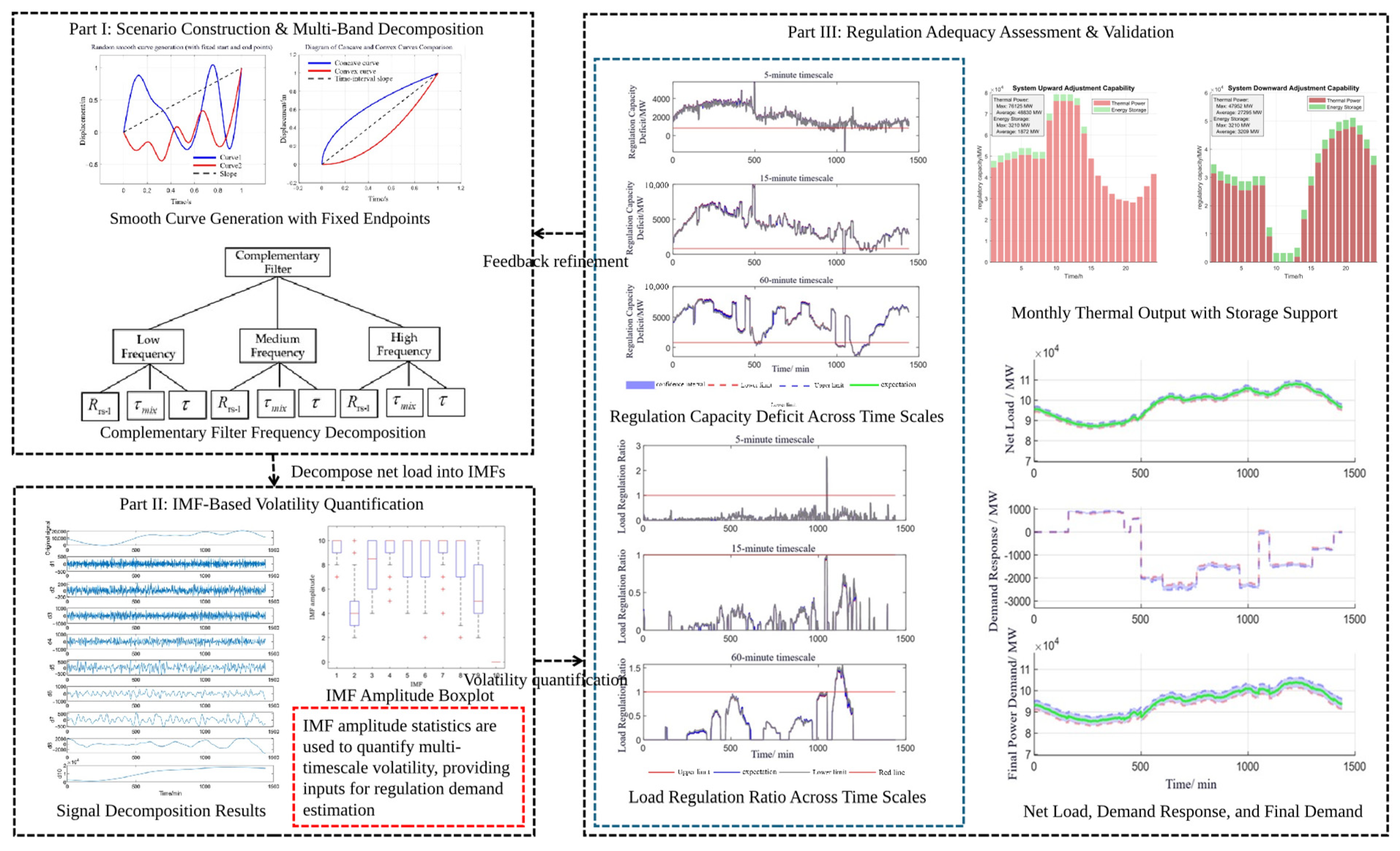
To more clearly articulate the research conducted in this paper, we present a framework diagram illustrating the complementarity between source and load and the capacity for regulation, as shown in
Figure 1.
2. Materials and Methods
Source-load matching refers to the degree of alignment between renewable energy output and load demand across three dimensions: temporal trends, fluctuation characteristics, and statistical distribution. Specifically, it encompasses the following: temporal matching reflects the synchrony of peak and off-peak periods in source-load curves; fluctuation matching characterizes the ability to track minute-to-hour-level variations; statistical matching quantifies collaborative risk features under extreme scenarios. Matching degree serves as a quantitative metric describing the system’s inherent supply demand coordination state, providing an objective benchmark for subsequent complementarity analysis. This definition positions matching as the foundational assessment step for complementarity, enabling precise characterization of source-load coordination characteristics to support in-depth analysis of system regulation requirements and balancing capabilities.
The matching characteristics between renewable energy output and load demand can be geometrically understood as the consistency of the change trends between the output curve and the load demand curve, including the direction and magnitude of change, temporal sequence of change, probability of simultaneous occurrence of maximum and minimum values, etc.; when source and load are completely matched, it means there is a translation relationship between the two curves; that is, their change trends are completely consistent.
2.1. Magnitude and Direction of Change
When ignoring the intermediate change process within the evaluation period, the magnitude and direction of change can be expressed by the slope at the start and end of the evaluation object as follows [
21]:
where
t is the current evaluation moment;
is the time scale of the evaluation period;
and
are the renewable energy output and load demand at time
t respectively;
and
are the slopes at the start and end of the renewable energy output and load demand curves within the
period respectively. Compared with expressing the direction and magnitude of change in percentages, using slopes has the advantage of eliminating the impact of inconsistent orders of magnitude between source and load, which is more in line with the original intention of the definition [
14].
The Pearson correlation coefficient can intuitively represent the normalized result of the linear relationship, but it can only evaluate the linear correlation through samples of two random variables. However, the calculation result of the slope is a scalar value. Therefore, Equation (2) is defined to normalize the correlation between the source and load slopes:
where
is the correlation between the slopes of the renewable energy output and load demand curves within the
period, used to measure the degree of linear correlation between the start and end points. Its value range is [−1, 1]. A value of 1 indicates that the slopes of the two curves are consistent, and a value of −1 indicates that the slopes of the two curves are opposite. This indicator reflects the linear correlation from another perspective.
2.2. Temporal Consistency of Change
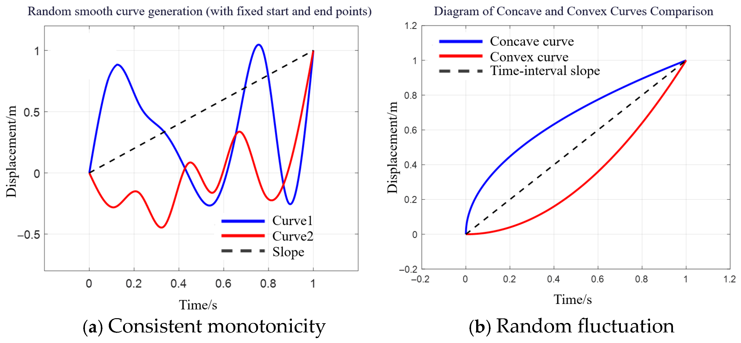
When analyzing with curve slopes, the intermediate change process between the start and end points is ignored. However, curves with consistent slopes within
may have very different intermediate change processes, as shown in
Figure 2.
Based on the ranks of data, the rank correlation coefficient can measure the monotonic relationship between the change trends of two variables and can be used to describe the temporal consistency of changes. Among them, the Spearman rank correlation coefficient sorts the observations of each variable separately and obtains the result by calculating the square of the rank difference of each pair of data points. It disrupts the order of samples and does not conform to the temporal characteristics of source-load changes; the Kendall rank correlation coefficient sorts each pair of observations, retains the temporal characteristics while being robust to small-sample data, and shows better ability in correlation evaluation on short time scales. Its probability expression is the following [
22]:
where
P{⋅} represents the probability of an event occurring;
and
are two independent data pairs, with
; the value range of
τ is [−1, 1]. A value of 1 indicates that the temporal change trends of the source and load curves are consistent, and a value of −1 indicates the opposite. It can be expressed numerically as below:
where
C represents the number of data pairs with consistent sorting directions of the two variables;
D represents the number of data pairs with inconsistent sorting directions of the two variables;
represents the correction term for duplicate values in variable X;
represents the correction term for duplicate values in variable Y; the correction term is the number of combinations of duplicate value groups in the observations, and the values are 0, 1, 2, …, n.
2.3. Tail Dependence of Change
Simply using the rank correlation coefficient for direct calculation can only obtain a numerical indicator measuring the monotonic relationship between variables and cannot describe the dependence differences in different regions. When two variables are highly correlated at extreme values but weakly correlated near the median, the rank correlation coefficient will average them, resulting in the loss of tail dependence. To fully capture the nonlinear and asymmetric complex relationships between two variables, the Copula function is used to describe the dependence structure between random variables. Based on Sklar’s theorem for continuous marginal distribution functions, there exists a unique Copula function that can connect the marginal distribution functions and the joint distribution function, as shown in Equation (5) [
23]:
where
is the joint distribution function of
random variables;
is the marginal distribution function of the i-th continuous random variable;
is the Copula function, describing the dependence structure between variables. To describe the complex dependence structure and tail correlation characteristics, a mixed Copula function is constructed by the convex combination of the empirical Copula, Gumbel Copula focusing on upper tail dependence, and Clayton Copula focusing on lower tail dependence:
where
is the non-parametric empirical Copula function;
is the Gumbel Copula with parameter
;
is the Clayton Copula with parameter
;
is weight parameters. In the evaluation of short periods,
is taken to emphasize tail dependence. It should be noted that since the Copula function calculation requires a large number of samples, a small sample size may lead to inaccurate estimation of the empirical Copula. The number of samples within the evaluation period is limited by the time scale and sampling frequency, which cannot meet the requirements. Therefore, it is necessary to combine a certain amount of historical data before the evaluation moment for estimation and then to perform rolling parameter estimation. The tail dependence obtained in this way can be expressed as follows:
2.4. Weakening of Sample Data Noise
There are many high-frequency, small-amplitude fluctuations in actual data, which will adversely affect the reliability of the rank correlation evaluation results. Filtering the original data will distort the results. To this end, this paper uses the method based on Improved Complete Ensemble Empirical Mode Decomposition with Adaptive Noise (ICEEMDAN) to decompose and reconstruct the original data to weaken the impact of noise [
24]. First, the first intrinsic mode of Gaussian white noise is added to the original signal to obtain the extended signal:
where
is the original signal;
is the extended signal;
is Gaussian white noise;
is the first mode component obtained using the ICEEMDAN method;
is the signal-to-noise ratio of Gaussian white noise to the original signal, and the value in this article is 0.2. Then, the first residual is calculated as shown in Equation (10):
where
is the first residual;
represents the calculation of the local average of the signal. The first mode is defined as follows:
where
is the decomposed first mode. After obtaining the first residual and the first mode, iterative update calculation can be performed:
where
is the
k-th residual;
is the decomposed
k-th mode. The predefined criterion for stopping iteration is to meet the maximum number of siftings or the residual component being a monotonic function.
After the decomposition of the original signal, all modes are divided into high-frequency, medium-frequency, and low-frequency categories for power reconstruction:
where
,
,
represent the reconstructed high-frequency, medium-frequency, and low-frequency signal components respectively;
and
represent the mode division numbers between high-frequency and medium-frequency signals, and between medium-frequency and low-frequency signals respectively, which are selected according to the number of mode decompositions—the values selected for
and
in this paper are 3 and 6, respectively.
2.5. Source-Load Complementarity Evaluation System
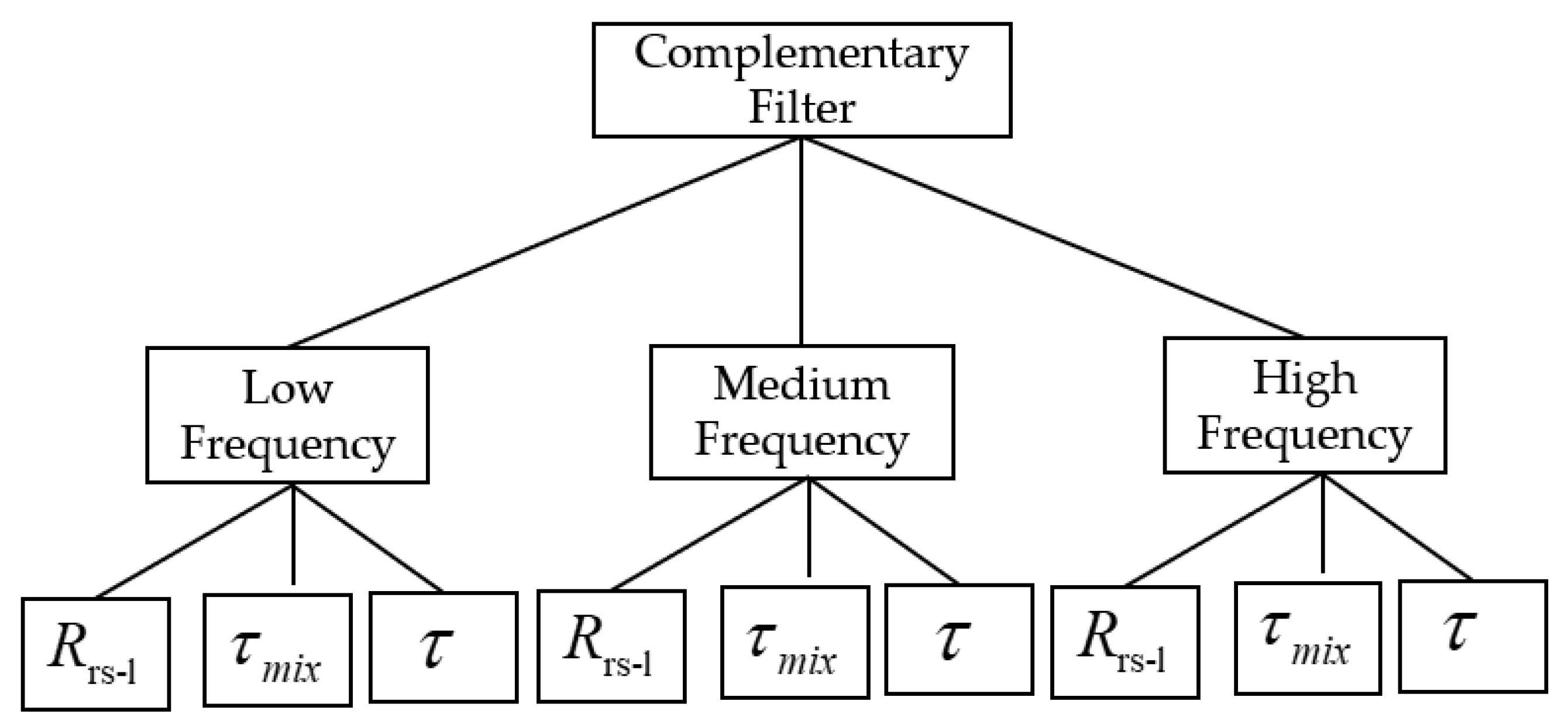
The Analytic Hierarchy Process (AHP) is used to construct the source-load complementarity evaluation system [
25], and its hierarchical structure is shown in
Figure 3.
Using the designed evaluation system structure, the complementarity results under the reconstructed signal components can be obtained:
where
is the quantitative complementarity result corresponding to each component;
are weight parameters, which are selected according to the degree of attention to each indicator. Then, the final quantitative evaluation result of source-load complementarity can be obtained by calculating the upper level.
2.6. Optimization Model
To conduct analysis of the resource regulation capabilities across multiple types, while linking to the results of the source-load complementarity evaluation in the previous section, this section establishes an economic model oriented toward optimal complementarity.
- (1)
Objective function
The objective function of the second stage considers the operation cost, investment cost, wind and solar power curtailment cost, and load loss cost. The expression is the following:
where
is the investment cost,
is the operation cost,
is the wind and solar power curtailment cost,
is the load loss cost.
- 1.
Investment Cost
The investment cost mainly considers the investment and construction cost of the new hydrogen storage tank:
where
is the investment cost per unit capacity of hydrogen storage tank;
is the planned capacity of hydrogen storage tank;
is the capital recovery factor;
r is the annual interest rate;
y is the average life of the tank device, about 20 years.
- 2.
Operating Costs
Operation cost includes fuel cost, unit operation depreciation cost, and startup cost:
where
is the fuel cost,
is the unit operation depreciation cost, and
is the fuel cost of the thermal power unit;
,
,
,
are the unit power operation costs of thermal power, renewable energy, electrolytic water devices, and fuel cell devices respectively;
is the power consumption of the electrolytic water device;
is the discharge power of the fuel cell device.
- 3.
Wind Power Curtailment Cost and Load Loss Cost
Wind and solar power curtailment cost and load loss cost refer to the penalty cost when power curtailment and power shortage occur:
where
is the penalty cost per unit of wind and solar power per unit of power abandonment, and
is the penalty cost per unit of power per unit of load loss.
2.7. Credible Capacity of Multi-Type Regulation Resources
The regulation capacity models of multi-type resources are shown in
Appendix A. The total regulation capacity model except for the load side can be obtained by aggregating the regulation capacities of the thermal power units and energy storage resources. Between two adjacent maintenance periods of the unit, considering the failure probability, each supporting power source or regulating equipment has two states during normal operation: forced outage and normal operation. When each unit meets the corresponding constraints, the probability distribution of its upward and downward regulation capacity can be expressed as follows [
26]:
where
and
are the maximum available upward and downward ramping capacities of unit
i at time
t respectively;
and
are the maximum upward and downward ramping capacities of unit
i respectively, with the subscript GE indicating the type of regulation resource;
,
, and
are the maximum rated output, minimum technical output, and current output of unit
i at time
t respectively;
is the forced outage probability of unit
i at time
t. With the continuous increase in the proportion of new energy access, the time scale requirement for regulation capacity evaluation in dispatch operation becomes shorter and shorter. Considering aging failures and random failures, the forced outage probability
can be expressed as below:
where the first term represents aging failure, and the second term represents random failure;
β is the shape parameter;
is the scale parameter, representing the characteristic life of the unit (the larger n is, the longer the aging life of the equipment);
t represents the operating time of the equipment, and its unit can be selected according to Δ
T;
λ is the random failure rate, following an exponential distribution, and the relevant parameters of common equipment are shown in
Table 1.
The available regulation capacity of a single unit follows a heterogeneous Bernoulli distribution with an extremely small
and has state dependence. At this time, the available regulation capacity of all adjustable units is the sum of the probability distributions of the available regulation capacity of each unit, and that is the following:
where
and
are the maximum available upward and downward ramping capacities of all units except the flexible load side at time t respectively; n is the number of all units; then both
and
follow a negatively skewed Poisson binomial distribution.
Due to the extremely small
, supporting resources are characterized by a large capacity of single units and a limited quantity, leading to the failure of the central limit theorem in describing the distribution of the total output of the units; at the same time, the fluctuation contribution of the output of each random variable (single unit) to the total output of all units is not sufficiently small, and the proportion of the variance of the output of a single unit to the total variance does not tend to 0, resulting in the failure of the Lindeberg condition. The extended form of the central limit theorem under independent but non-identical distributions cannot be used. To avoid the loss of tail probability caused by underflow due to low-order term truncation, the recursive method is used to accurately calculate the probability mass function of the available regulation capacity of all adjustable resources:
where the symbol “
” represents the convolution operation. Based on the obtained accurate distribution function, by sorting the available regulation capacity of all adjustable units in ascending order and accumulating the sum can obtain its cumulative distribution function:
where
and
are all possible sums of the maximum available upward and downward ramping capacities of all adjustable resources at time
t respectively. Based on the cumulative distribution function, the corresponding confidence interval can be obtained by selecting the significance level
α.
The expectations of
and
can be calculated using Equations (23) and (24):
where
represents the expectation of the variable.
2.8. Fluctuation Domain of Net Load
This section introduces the Minkowski sum to construct a deterministic range for net load fluctuations, serving as a unified boundary for subsequent hierarchical evaluations. Its physical significance lies in characterizing the extreme potential range of net load fluctuations across all possible phase combinations within the uncertainty set of sources and loads.
Core considerations are as follows:
- (1)
In the absence of precise joint distributions, it provides a deterministic alert zone covering the most unfavorable superimposed scenarios for dispatch.
- (2)
This range serves as an input benchmark for subsequent probabilistic convolution modules to perform refined resource matching and reliable capacity assessment, facilitating the transition from deterministic boundaries to probabilistic decisions.
- (3)
When input data include extreme scenarios, the constructed interval automatically encompasses these cases. Since this study’s input data originate from time-series simulations containing extreme scenarios, the interval inherently possesses the capability to represent extreme events.
- (4)
This study adopts a layered framework: the first layer provides deterministic full-coverage boundaries, while the second layer performs probabilistic refinement analysis. This forms a combined strategy of “boundary delineation + internal assessment,” balancing safety benchmarks and decision-making information dimensions.
In a power system with large-scale and high-proportion new energy, its power balance can be described as follows [
27]:
where
,
,
,
,
,
,
and
are the outputs of coal-fired power generation, gas-fired power generation, hydropower, wind power, PV power, energy storage systems, actual load after response, and nuclear power r at time t respectively. The symbol is positive when the energy storage system supplies power to the grid and negative when it absorbs power from the grid;
,
,
,
,
,
and
, are the total numbers of coal-fired power generation, gas-fired power generation, hydropower, wind power, PV power, energy storage systems, and nuclear power respectively. Among them,
is the sum of the load forecast value and the demand response capacity as follows:
where
is the load forecast value at time
t.
The net load can be expressed as below:
where
is the system’s net load at time
t, that is, the demand after deducting renewable energy output from the sum of actual load and line loss. When the power balance is satisfied, its value is equal to the power generation load of the supporting power sources and energy storage. Since the line loss fluctuation is much smaller than the load fluctuation and the new energy output fluctuation, it can be ignored when analyzing volatility. At this time, the uncertainty of the net load is mainly composed of the superposition of the uncertainty of load demand and the uncertainty of new energy output, such as wind power and PV power. When considering uncertainty for analysis, the possible values of load demand and new energy output at time
t + Δ
T are both bounded sets. At this time, the superposition of their fluctuation domains is the fluctuation domain of the net load, that is, the Minkowski sum of their fluctuation domains is calculated:
where
,
,
and
are the fluctuation domains of the system’s net load, total load demand, wind power output, and PV output at time
t + Δ
T respectively;
,
,
and
are the first-order differences of each power value from time
t to
t + Δ
T respectively. Since the fluctuation domain expands once for each Minkowski sum operation, if the fluctuation domain of each new energy station is taken as the summation object, although it seems refined, the boundary of the fluctuation domain will expand excessively after multiple Minkowski sum operations, making it meaningless for analysis. To ensure the boundedness and usability of the fluctuation domain, this paper selects the fluctuation value set of the total wind power, PV power, and load as the operation object, which is data that can be easily obtained in the dispatch system.
The manifestation of the power values of new energy and load at time
t + Δ
T may be as follows: ① probability density function and confidence interval for probabilistic prediction; ② a fixed value for deterministic prediction; ③ discrete data set for multiple repeated predictions. The expectation and confidence interval of the fluctuation domain in each case can be calculated in the following ways: ① the expectation and confidence interval of the fluctuation value are obtained by subtracting the power value at time
t from the expectation and confidence interval of
; ② when the predicted value is taken as the expectation, the sample statistical confidence interval of the fluctuation value in similar scenarios at the same period in the past is used; ③ the expectation of discrete samples is calculated, and the confidence interval of the fluctuation value is obtained by subtracting the power value at time
t from the sample confidence interval. Taking the manifestation as the probabilistic prediction result as an example, the probability density functions of the power values of new energy and load at time
t + Δ
T are known, then the probability density functions of the fluctuation values at time
t + Δ
T are the following:
The probability distribution of the net load fluctuation domain is as follows:
The expectation and confidence interval of the net load fluctuation value can be obtained using the calculation result of Equation (37).
2.9. Quantitative Evaluation of Regulation Capacity
The system’s regulation capacity can be conveniently quantitatively evaluated using the credible capacity of multi-type regulation resources and the expectation and confidence interval of the net load. For dispatch, it is necessary to know the regulation capacity indicators under different time scales and the matching degree of regulation capacity to the net load fluctuation value to arrange unit start-up and shutdown. Since the fluctuation frequency of new energy output is much higher than that of regulation capacity, the load regulation ratio and ramping capacity adequacy margin indicators are defined to quantitatively evaluate the system’s regulation capacity under each evaluation state [
28].
- (1)
Load Regulation Ratio in Upward Ramping State
where
,
and are the matching capacities of the credible upward ramping capacity of regulation resources to the net load fluctuation under the expectation, confidence lower limit, and confidence upper limit evaluation states after the evaluation time scale Δ
T starting from time
t respectively;
and
are the confidence lower limit and confidence upper limit of the variable at the significance level
α respectively. This indicator can obtain the intuitive quantitative results of the matching capacity of regulation resources to the net load fluctuation under each evaluation state within the evaluation period. A lower load regulation ratio indicates that the credible capacity of regulation resources is more sufficient relative to the net load fluctuation, with a larger regulation margin.
- (2)
Upward Ramping Capacity Adequacy Margin
where
,
, and
are the adequacy margins of the credible upward ramping capacity of regulation resources and the net load fluctuation under the three evaluation states of expectation, confidence lower limit, and confidence upper limit after the evaluation time scale Δ
T starting from time
t respectively, that is, the nominal value of excess or shortage of regulation capacity after Δ
T, which is directly used to guide unit start-up and shutdown.
2.10. Optimization Variables and Optimization Methods
Since the optimization objective function of this model is linear and all constraints have been linearized, the model constitutes a linear programming (LSP) problem. To solve this LSP optimization problem, we employed the commercial solver Gurobi 10.0. This model is a mixed-integer linear programming (MILP) model. Solver parameter settings include: MIPGap set to default value le-4; TimeLimit set to 3600 s. All simulations were executed on a computer equipped with an Intel CoreTM-i7-14700HX processor (2.4 GHz) and 64 GB of memory.
The optimization variables and objectives addressed in this paper are presented in
Table 2, encompassing both direct and indirect optimization variables.
3. Results and Discussion
Considering the daily periodic variation characteristics of PV output, this paper uses the measured minute-level data of a typical day in a provincial power grid for case verification and analysis.
Referring to the composite weights proposed in
Section 2.4, we calculated the weights for indicators
,
, and
using the entropy weight method based on six sets of actual sub-indicators. The resulting weight values are 0.2147, 0.3442, and 0.4411, respectively. As the entropy weight method is a common approach for calculating weights based on measured data, further details are omitted here. The specific six sets of actual data are presented in
Table 3.
For specific data related to the calculation example, refer to
Table 4.
3.1. Analysis of Optimization Results
The optimized results of this study are shown in
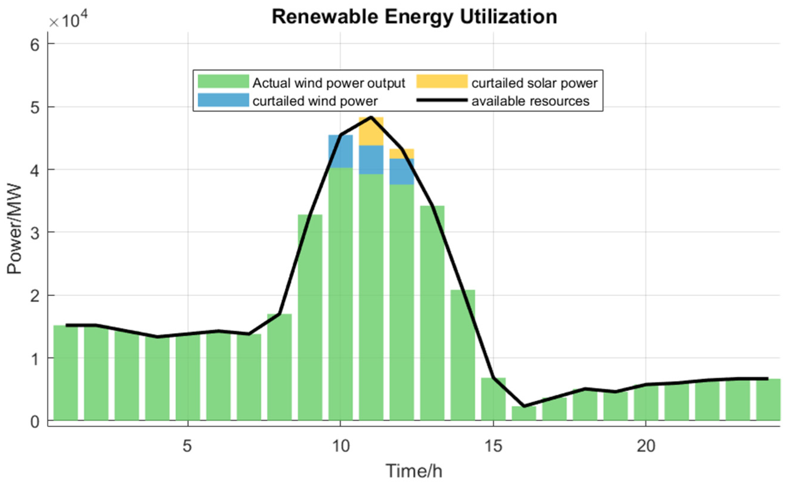
Table 5 below. The total system cost amounts to 513,051.42 million yuan, with no power shortages occurring. There was 20,009.37 MW of curtailed electricity, representing a curtailment rate of 5.1%.
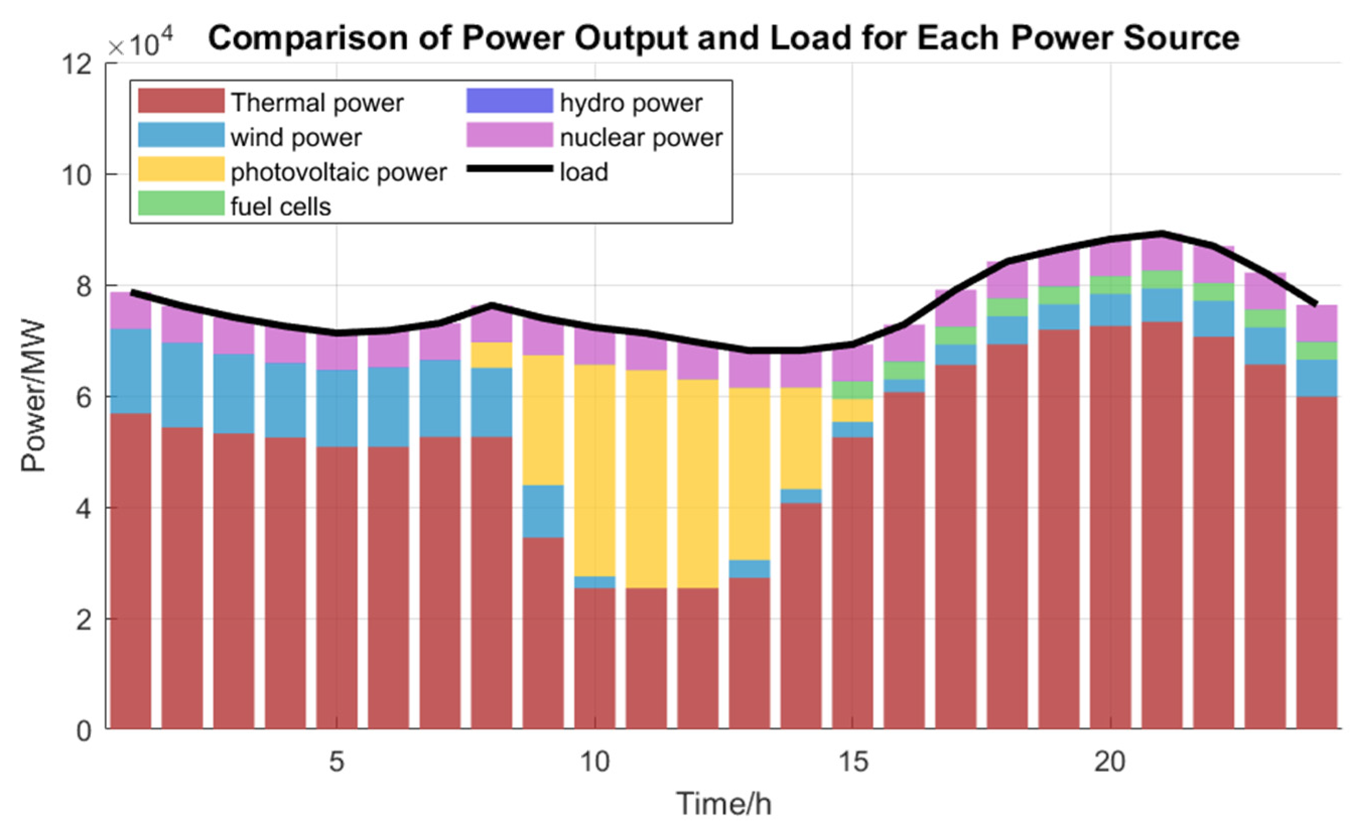
Analysis results based on the 24 h time-series optimization model indicate that the multi-resource power system achieved precise power balance during a typical day (See
Figure 4). Total generation of 1831.71 GWh perfectly matched total load, with a net power difference of zero, ensuring stable and reliable system operation. Thermal power units, serving as the dominant power source, contributed 1264.07 GWh of generation, accounting for 69.01% of the total, demonstrating their foundational load support role within the power system. Renewable energy sources demonstrated outstanding performance, with wind and solar power accounting for 20.51% of total output. However, the 20,009.37 MWh of curtailed electricity highlighted integration challenges stemming from their intermittency. Maximum curtailment power reached 9088.20 MW, with a curtailment rate of 10.89%, primarily occurring during periods of excess wind and solar resources coupled with constrained system regulation capacity. Nuclear and hydroelectric power, as stable sources, contributed 8.66% and 0.07% of generation respectively, further enhancing system reliability. Fuel cell systems exhibited continuous discharge characteristics, with a total 24 h discharge of 32.10 GWh, playing a crucial role in flexibility regulation.
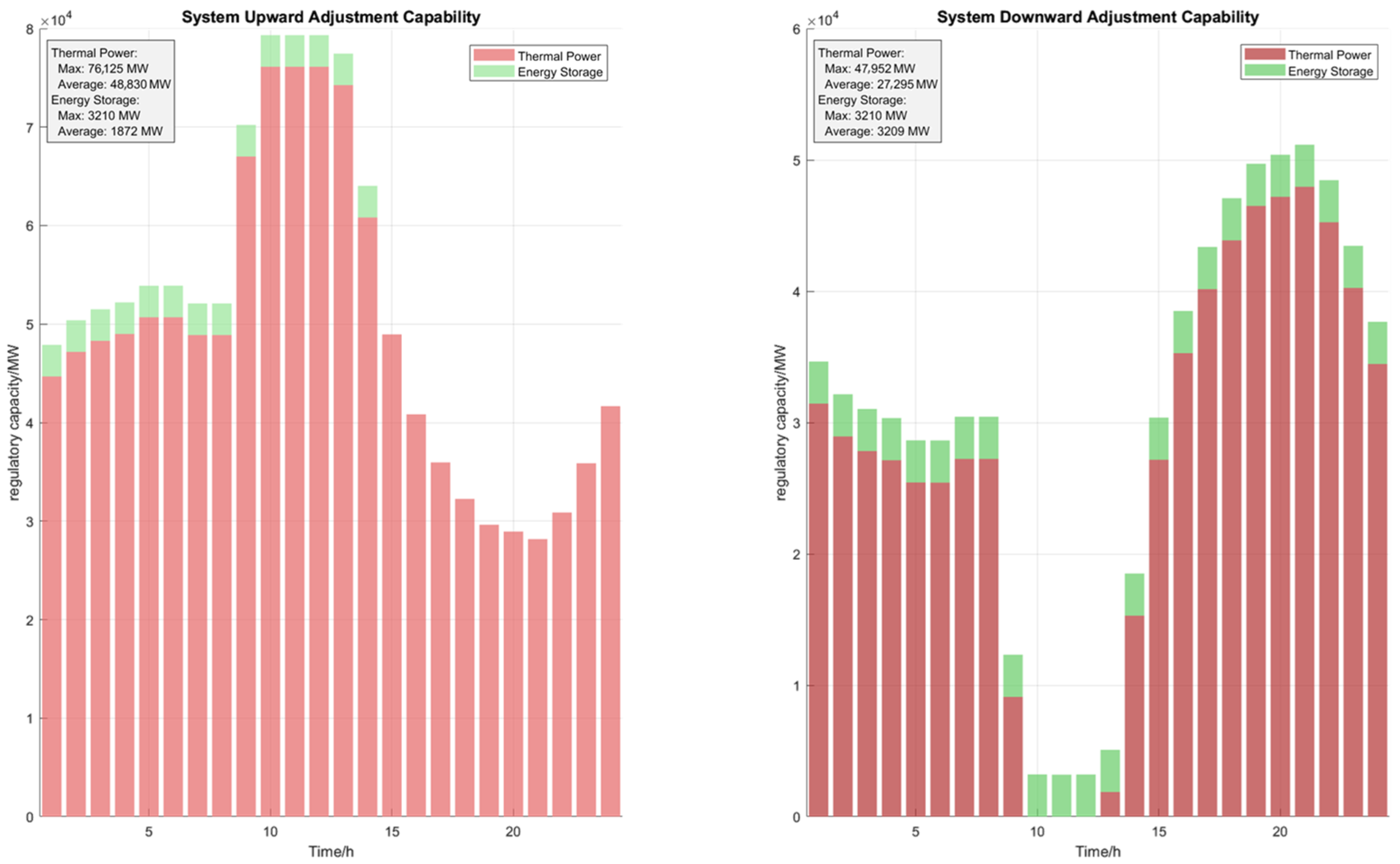
System regulation capacity assessments revealed significant bidirectional regulation potential in thermal units, with average upward regulation capacity reaching 48.83 GW and downward capacity at 27.30 GW (See
Figure 5). This stems from the ample operational margin between their 101.5 GW installed capacity and minimum technical output of 25.375 GW. While fuel cell systems exhibit relatively limited regulation capacity, they demonstrate rapid responsiveness with an average upward regulation capacity of 1.87 GW, offering unique advantages in short-term power regulation. Notably, despite the system’s overall adequate regulation capacity, significant curtailment persists. This highlights room for optimizing operational strategies: during periods of high wind and solar generation, the system fails to fully utilize all available adjustable resources to absorb excess electricity. While this may stem from economic considerations, optimizing dispatch strategies could further enhance renewable energy utilization efficiency.
Through quantitative analysis of the output from each power source in
Figure 1, it is evident that the system load demand exhibits a pronounced peak-to-trough difference. Thermal power output remains at a relatively high level, serving as the core for ensuring the base load. The output curves of wind and solar power show a weak correlation with the load curve, particularly during peak load periods when their output is limited. This indicates that their intermittency significantly impacts the system’s net load curve, increasing the pressure on system dispatch. As shown in
Figure 2, the renewable energy utilization rate reveals a persistent gap between the “available resource” curve and the “actual output” curve for wind and solar power, with particularly significant discrepancies during certain periods corresponding to curtailed wind and solar power. This quantifies the waste of clean energy caused by factors such as grid absorption capacity limitations, insufficient system flexibility, or transmission constraints. The data indicate that enhancing system flexibility and optimizing real-time dispatch are key to improving renewable energy utilization rates and reducing curtailment.
3.2. Analysis of Source-Load Complementary Characteristics
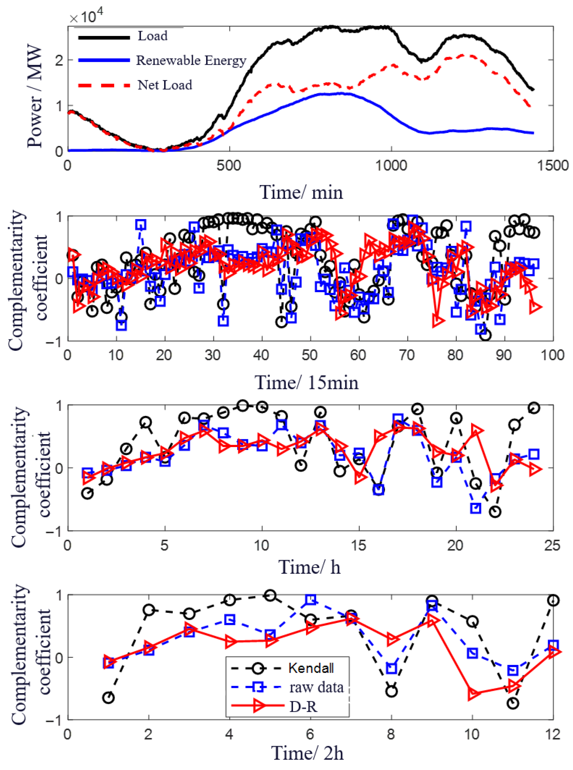
To facilitate the observation of the consistency of source-load change trends, the original data are processed to the same dimension while maintaining their respective trends. Three methods are selected for comparison: directly calculating the Kendall correlation coefficient for the original data, using the proposed complementarity evaluation method for the original data, and using the proposed complementarity evaluation method after data decomposition and reconstruction, under the three time scales of 15 min, 1 h, and 2 h. The results are shown in
Figure 6.
It can be seen from
Figure 6 that the results of directly calculating the Kendall correlation coefficient for the original data are prone to maximum or minimum values on short time scales, indicating that the change trends of new energy and load are highly consistent or opposite, which is inconsistent with the trends of the actual curves; the results of using the proposed complementarity evaluation method for the original data show that the probability of extreme values is reduced, but extreme values are still prone to occur in the complementarity evaluation on short time scales; the proposed complementarity evaluation method after data decomposition and reconstruction improves the accuracy of the complementarity evaluation results reflecting the consistency of source-load change trends while retaining the true characteristics of the original data, and has better adaptability to small time scales. When the net load value is relatively stable, the complementarity coefficient shows a large positive value, which proves the correctness of the complementarity quantification.
3.3. Decomposition of Net Load Signals and Noise Mitigation Analysis Based on ICEEMDAN
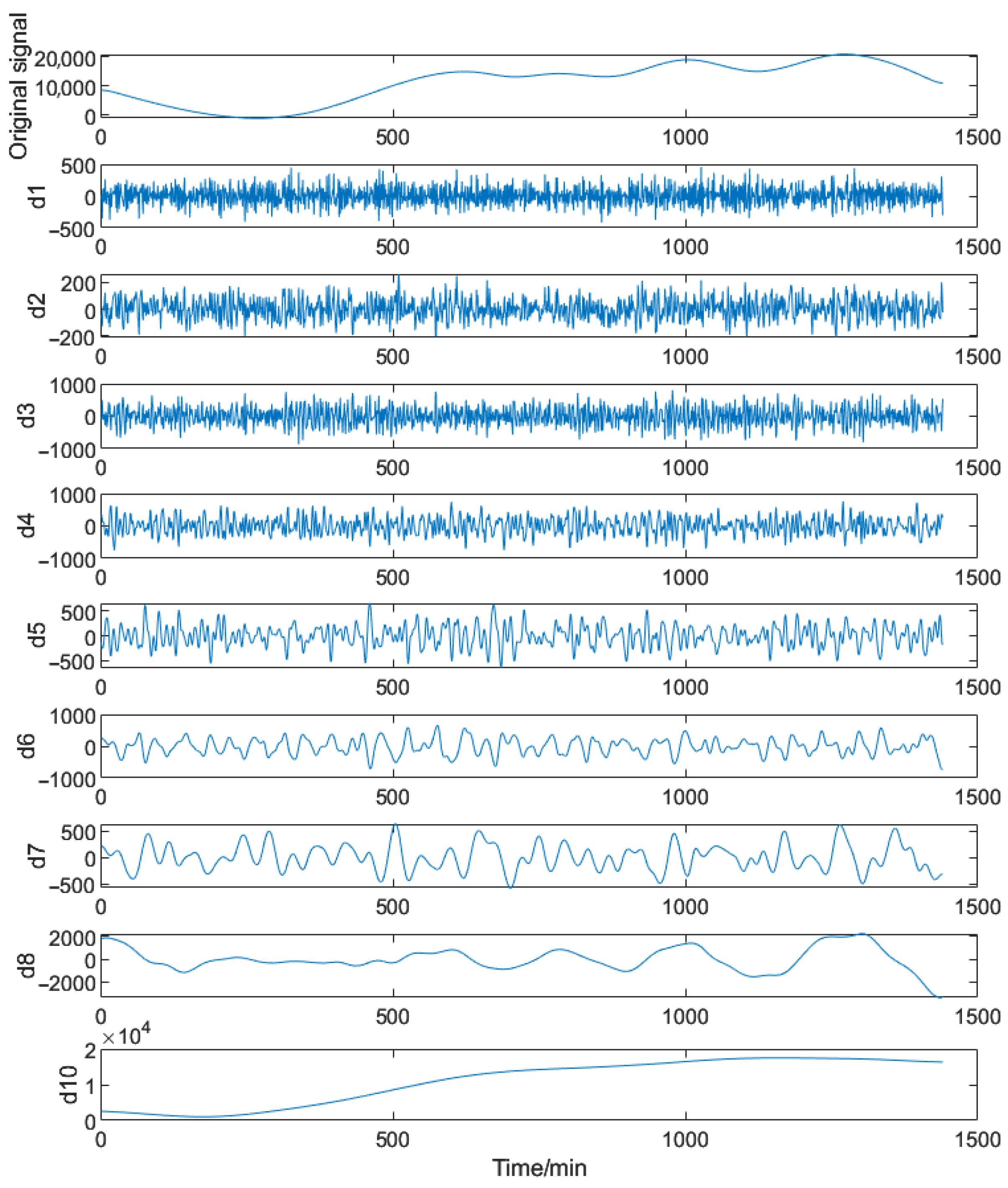
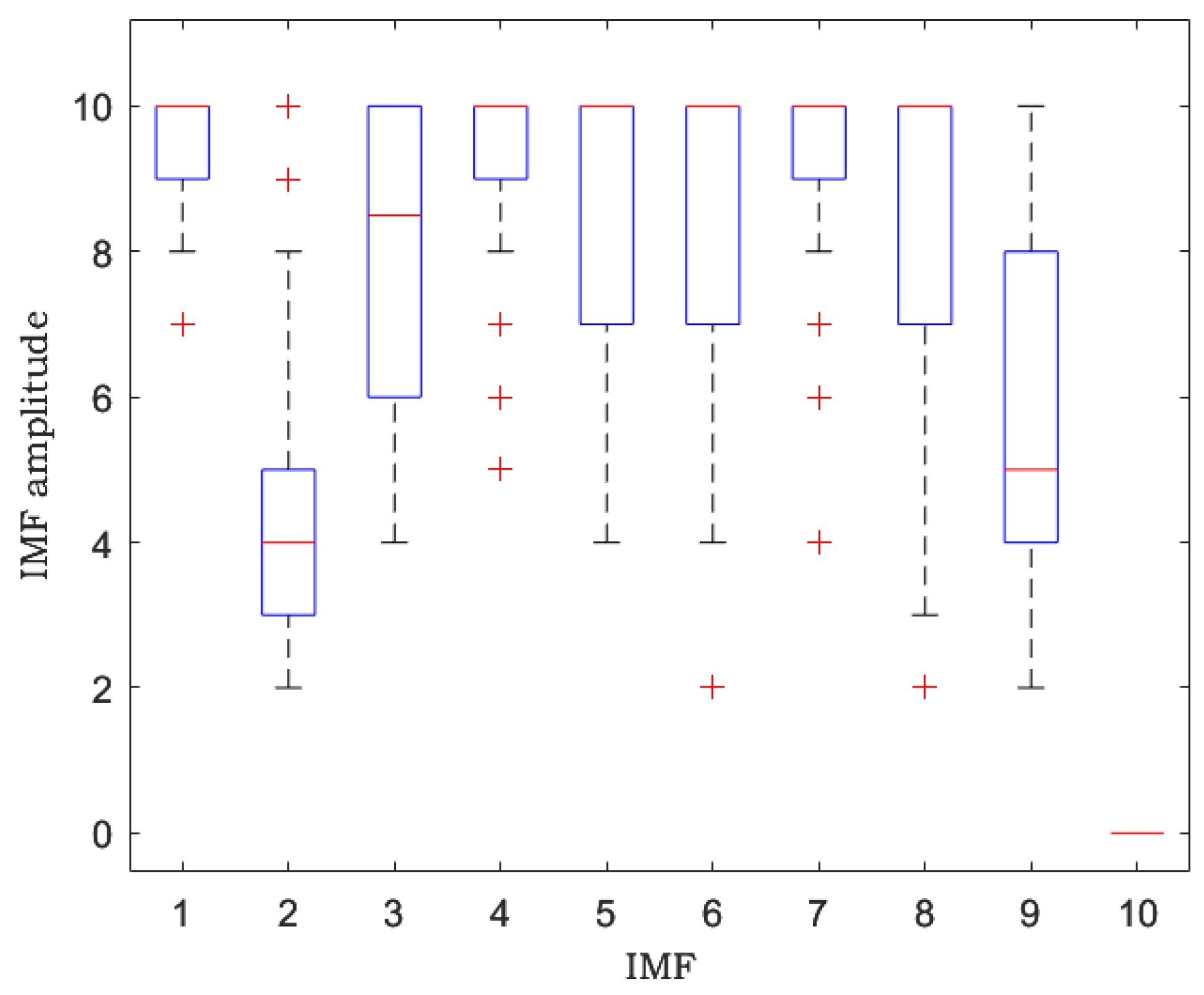
This paper employs the improved adaptive noise-complete set empirical mode decomposition (ICEEMDAN) method to decompose and reconstruct net load time series data. This method adaptively decomposes signals into a series of intrinsic modal functions ranging from high to low frequencies based on the data’s inherent characteristics, thereby separating noise from the effective signal. The decomposed components are shown in
Figure 7, with corresponding box plots presented in
Figure 8.
Following ICEEMDAN processing, the original net load signal is decomposed into a total of nine IMF components (d1–d9). Based on the frequency characteristics and physical significance of each component, this study focuses on in-depth analysis of three representative components: IMF1 (d1) representing high-frequency noise, IMF4 (d4) reflecting intraday core fluctuation patterns, and IMF9 (d9) embodying long-term trend changes.
First, IMF1 (d1) exhibits narrow oscillations between 19.8 and 23.5, with its time series curve displaying rapid, disordered fluctuations. The corresponding box plot reveals significant dispersion and numerous outliers, consistent with the typical statistical characteristics of high-frequency random noise. This constitutes the primary interference component requiring attenuation in the signal. Second, IMF4 (d4), representing the mid-frequency component, exhibits a regular decreasing trend from −100 to −400 over the time interval, with smooth and continuous variation. Its box plot features a short box and high data concentration, indicating that this component carries the stable, predictable core fluctuation pattern of net load within the daily cycle. It serves as a key information carrier for analyzing load characteristics. Finally, IMF9 (d9), representing the low-frequency trend component, exhibits a slow, smooth variation within the range of 99.8 to 109.8. Its box plot shows a distinct upward shift, clearly delineating the baseline load level and gradual trend evolution of net load throughout the day. This component forms the foundational layer determining the overall load trajectory.
This paper applies the ICEEMDAN method to effectively decompose the net load signal, identifying three core components: noise, primary oscillatory patterns, and long-term trends. This lays a solid foundation for subsequent research.
3.4. Analysis of Regulation Capacity
Figure 9 below shows the upward and downward regulation capabilities of the optimized power system on a typical day. System regulation capacity increases over time, with thermal power serving as the primary upward regulation force, rising from 45,000 MW at 00:00 to 74,000 MW at 52:00. Energy storage provides significant downward regulation capacity, stabilizing at 35,000 MW after 01:00 and maintaining consistency across all time periods. This effectively complements thermal power regulation capacity, enhancing the system’s flexibility in responding to net load fluctuations.
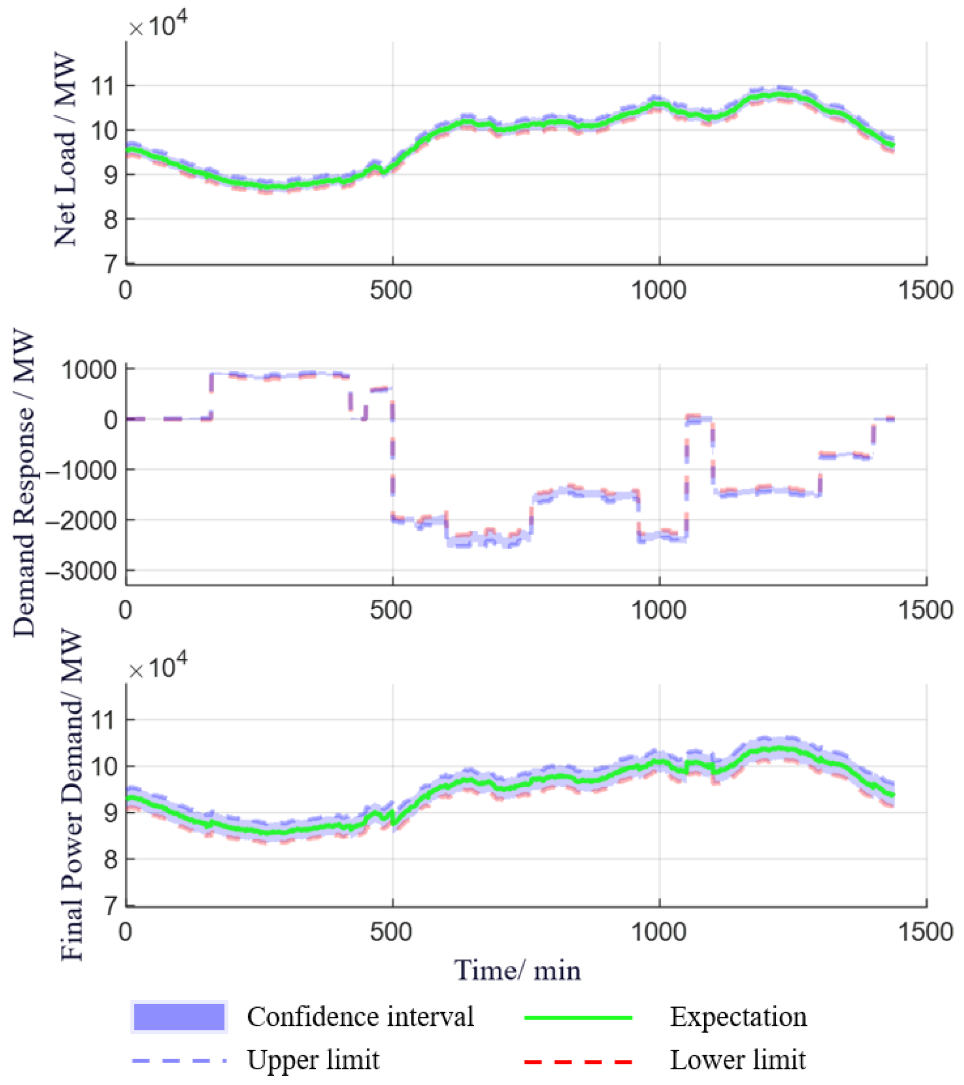
Taking upward ramping as an example, the intraday distribution of the net load considering demand response is obtained by applying the proposed analysis method, as shown in
Figure 10. After considering demand response, the fluctuation range of the final load demand relative to the controllable regulation resources will increase; similarly, the credible capacity of regulation resources aggregated by thermal power and energy storage can be obtained (due to space limitations, it is not listed here).
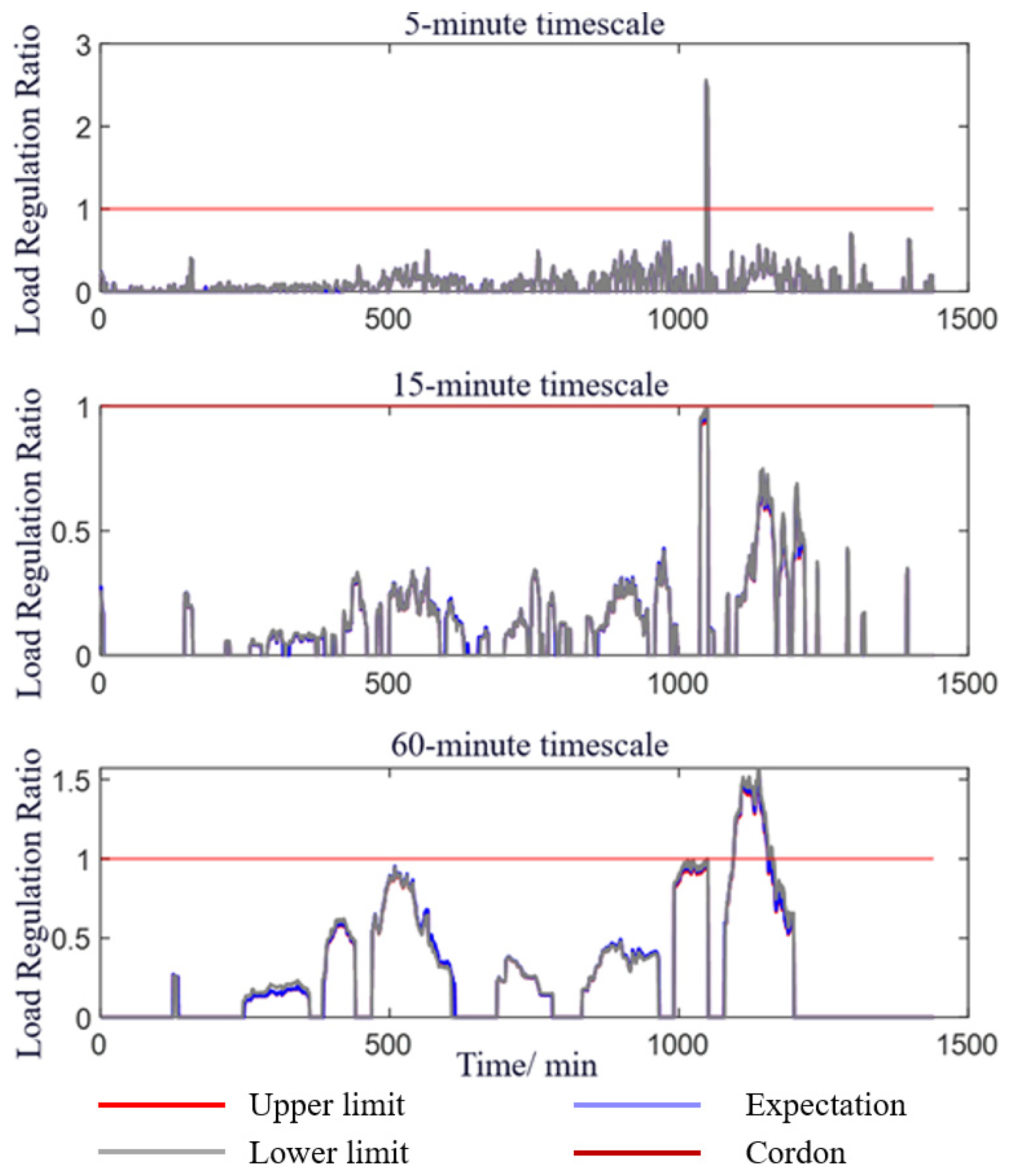
By comparing and analyzing the final load demand with the credible capacity of regulation resources, the intraday change curves of the load regulation ratio in the upward ramping state under different time scales are obtained, as shown in
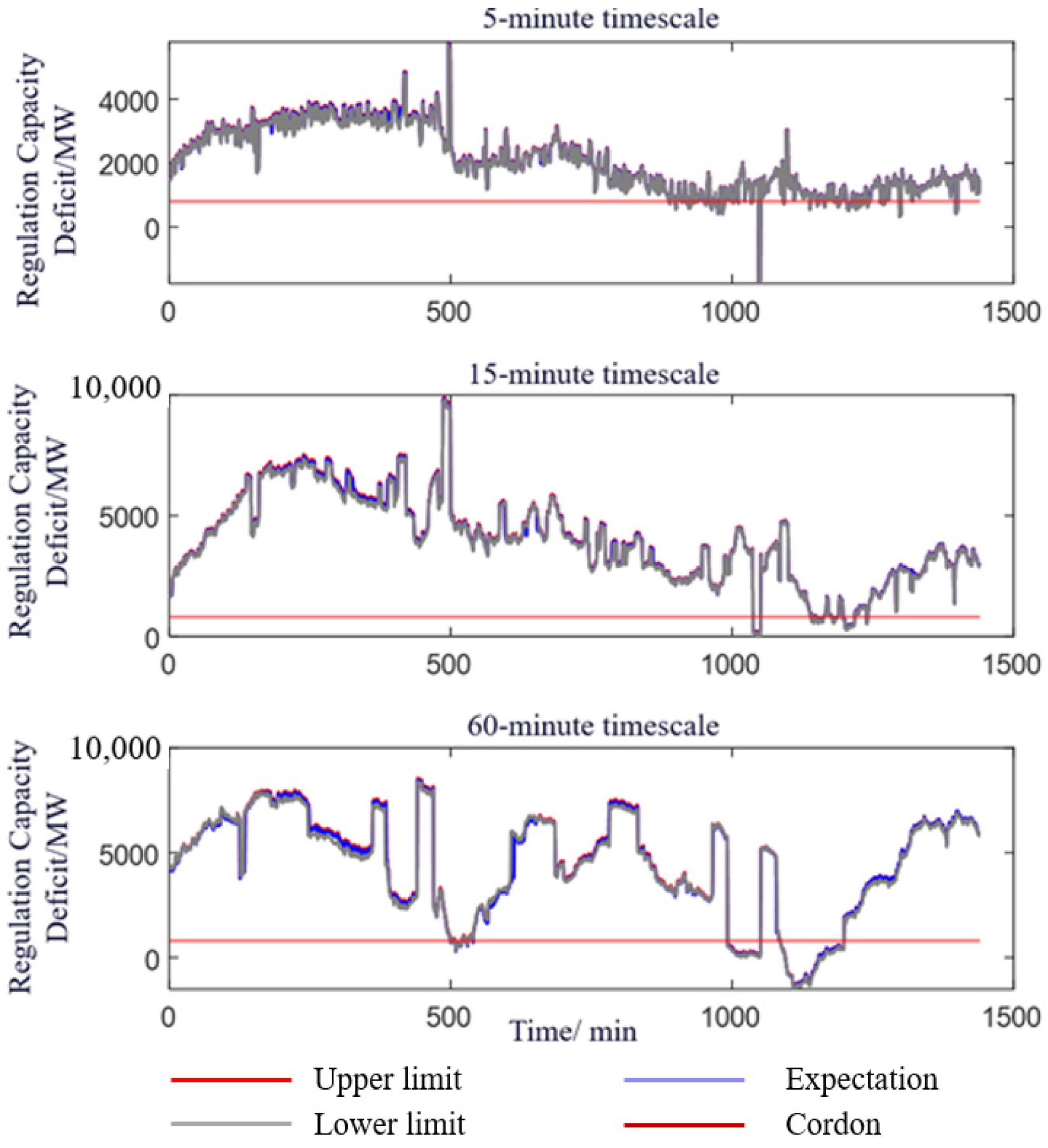
Figure 11, and the intraday change curves of the upward regulation capacity adequacy margin are obtained, as shown in
Figure 12.
On the 5 min time scale, the final net load fluctuation during the evening peak period will exceed the regulation capacity of the regulation resources under the three evaluation levels of confidence upper limit, expectation, and confidence lower limit, which is also reflected on the 60 min time scale. The regulation capacity adequacy margin at the corresponding moment can be given specific values, as in
Figure 12. On the 15 min time scale, although there is no shortage of regulation capacity throughout the day, it has approached the upper limit of the credible capacity of regulation resources during the evening peak period, with a risk of shortage. The load regulation ratio on the 60 min time scale is more likely to reach the warning value compared with the 5 min and 15 min time scales. This is because the thermal power units have reached their output limits after 60 min, while energy storage, although close to instantaneous response, has a limited duration of action. Therefore, when the final net load is in a state of continuous increase or decrease, the longer the time, the higher the probability of insufficient regulation capacity.
Taking the upward regulation capacity and regulation capacity adequacy margin on the 5 min time scale as examples, the conventional maximum regulation capacity is selected as the comparison benchmark, and the comparison results are shown in
Table 1. The maximum differences between the proposed method and the maximum regulation capacity under the three levels of confidence upper limit, expectation, and confidence lower limit are −2.845 MW, −55.58 MW, and −108.5 MW, respectively, and the maximum differences of the corresponding regulation capacity adequacy margin are −29.31 MW, −62.67 MW, and −705.9 MW, respectively (
Table 6). It can be seen that the maximum differences under both the expectation and confidence lower limit evaluation levels have already had an impact on the unit commitment.
4. Conclusions
This paper first analyzed the definition perspective and evaluation method of source-load complementarity in existing studies and proposes a source-load complementarity evaluation method suitable for multi-time scales based on the source-load matching idea. Then, considering the net load fluctuation domain and the failure probability of source-side units, a quantitative evaluation method for regulation capacity under confidence levels is proposed. The main conclusions are as follows:
Defining complementarity from the perspective of source-load matching is more in line with the dispatch perspective. High-frequency, small-amplitude fluctuation signals have an adverse impact on the rank correlation evaluation, which is likely to cause deviations in the evaluation results.
In the evaluation of regulation capacity at future moments, it is necessary to consider the fluctuation domains and their confidence intervals of load and new energy. Compared with the evaluation method based on maximum regulation capacity, the credible capacity method proposed in this study can more truly reflect the regulation capacity under multiple uncertainty factors.
The accuracy of the proposed source-load complementarity evaluation method was verified through a case study. The differences in regulation capacity adequacy under different evaluation levels were compared and analyzed, which can be used to support unit commitment and provide more perspectives for the evaluation of regulation capacity.
In the future, the planning and configuration method of new types of regulation resources under different evaluation levels will be further considered.