Article

Research on Characterization and Detection Methods of Photovoltaic Cell Thermal Defects Based on Temperature Derivatives

1
School of Electrical Engineering, Southwest Jiaotong University, Chengdu 611756, China
2
State Grid Zhejiang Electric Power Company–Yiwu Power Supply Company, Yiwu 322000, China
*
Author to whom correspondence should be addressed.
Inventions 2026, 11(1), 14; https://doi.org/10.3390/inventions11010014
Submission received: 25 December 2025 / Revised: 12 January 2026 / Accepted: 19 January 2026 / Published: 4 February 2026

Abstract

Photovoltaic (PV) cells play an important role in the development of green energy. However, in practical photovoltaic systems, shunting-related defects and hotspot phenomena may originate not only from manufacturing imperfections, but also from mechanical stress and environmental factors during transportation, installation, and long-term field operation. Such hotspots not only reduce the power-generation efficiency and service life of PV cells but may also pose safety risks to grid-connected photovoltaic power stations. To address this problem, a squared even-order derivative (SEOD) method based on surface temperature analysis is introduced to enable the quantitative detection of thermal defects in PV cells. In this study, typical faults in PV cells, including low-resistance defects and silicon-based deep scratches, are analyzed. A simulation model is established to correlate typical faults with their equivalent volumetric heat sources, followed by experimental validation for low-resistance defects. Based on this framework, the SEOD algorithm is developed and applied to achieve high-precision localization and quantitative characterization of thermal defects in both simulation models and experimental samples.

1. Introduction

Solar energy is widely regarded as a clean and sustainable energy source with abundant availability, which has driven the rapid development of photovoltaic power generation technologies in recent years. In an ideal PV cell, the current density on the silicon substrate is spatially uniform [1]. In practical PV cells, however, deviations from this ideal condition inevitably occur due to defects introduced during fabrication as well as mechanical stresses encountered in the field. Typical manufacturing-related defects include deep scratches formed during silicon laser cutting and low-resistance shunts caused by cracks in pre-metallization screen printing [2,3,4]. Similar defect characteristics can also develop during transportation, installation, and long-term operation as a result of mechanical and environmental loads [5]. All these defects can lead to severe ohmic shunting and localized heating of the silicon substrate [6]. The accumulation of heat over a long period of time not only degrades the power generation efficiency of the solar cell [7], but also damages its physical structure [8]. In particular, when a low-resistance defect in part or all of a solar cell is masked, damaged, or becomes electrically incompatible and enters a reverse-bias state, the thermal dissipation power increases sharply, eventually leading to irreversible and severe consequences [9,10]. Table 1 presents long-term operational data from three photovoltaic plants, demonstrating overall power degradation and the frequent occurrence of defect-related phenomena such as scratches and hotspots. These observations suggest that, although power degradation in photovoltaic power plants is typically driven by multiple degradation mechanisms, defect-related hotspot issues are prevalent in long-term operating modules, and their detection and characterization have independent and significant engineering value.
Detection methods for PV cell defects usually include voltammetric characteristic curve (V-I) analysis [12], electroluminescence (EL) imaging [13], and visual inspection. Infrared thermography (IRT), as a non-destructive testing technique used to measure the surface temperature of an object, thereby assessing the thermal state of a device [14], has attracted considerable research interest for defect detection and assessment of PV module classification [15,16]. In particular, early studies have demonstrated that defect-related heat sources and their spatial characteristics can be analyzed through thermal modeling and infrared measurements, thereby providing a physical basis for thermographic defect localization [17].
Various IRT-based techniques have been developed for PV defect inspection, including electrical pulsed infrared thermography (EPIT) [18], electromagnetic induction infrared thermography (EIIT) [19], and lock-in thermography (LIT) [20,21]. In addition, spatial derivative-, gradient-, and resolution-enhancement approaches have been explored to improve defect visibility and localization accuracy in thermographic images [22,23].
However, as the scale of photovoltaic power plants continues to increase, the large number of PV cells, together with the multiple procedures, high costs, and strict operating conditions associated with these methods, limit the feasibility of existing IRT-based non-destructive techniques for economical and large-scale PV defect inspection [24]. Beyond these practical constraints, many existing thermographic and derivative-based approaches remain primarily qualitative, providing limited capability to quantitatively relate observed thermal features to underlying defect parameters. These limitations highlight the need for an improved diagnostic approach.
Therefore, this study presents a squared even-order derivative (SEOD) method for the detection and characterization of thermal defects in PV cells. Rather than aiming to repair failed modules, which typically require replacement once severe degradation has occurred, the proposed method focuses on improving diagnostic capability at the defect detection stage. Compared with conventional infrared thermography, which mainly provides qualitative hotspot identification, the SEOD approach enhances spatial localization and enables quantitative characterization of defect-related thermal anomalies. In contrast to existing gradient- or derivative-based thermographic techniques that are primarily used for contrast enhancement or qualitative feature extraction, the SEOD method systematically exploits specific even-order derivative responses to establish a direct quantitative relationship between surface temperature features and defect parameters. This enhanced diagnostic capability supports condition assessment and more informed maintenance or replacement decisions, particularly in large-scale photovoltaic installations.
This study presents the SEOD method, which retains the inherent advantages of non-destructive testing while streamlining operational procedures to enhance practical applicability. Two representative fault simulation models for conventional solar cells were developed, with experimental validation conducted specifically on the low-resistance defect model. Subsequent investigation focused on the key side-peak characteristics of the even-order derivative of PV cell surface temperature. A mathematical relationship was established to correlate the position and severity of thermal defects with the derivative profile, enabling quantitative defect identification. The methodology was further applied to a simulation model of PV cells incorporating thermal defects. Experimental results demonstrate the method’s capability to achieve both visual spatial resolution and quantitative detection of thermal anomalies. Finally, thermal defect detection was performed on low-resistance experimental samples. The favorable outcomes confirm the method’s effectiveness and feasibility in practical application scenarios.
The rest of the paper is organized as follows. Section 2 presents the finite-element modeling of thermal defects in PV cells and establishes equivalent volumetric heat-source models for typical defects, followed by the methodology of the squared even-order derivative (SEOD) approach. Section 3 reports and discusses the simulation and experimental results to validate the proposed method in terms of defect localization and quantitative characterization. Finally, Section 4 concludes the paper and summarizes the main findings.

2. Materials and Methods

2.1. Finite Element Modeling of Thermal Defects in PV Cells

2.1.1. Physical Model

The typical structure of a solar cell consists of multiple layers of different materials stacked on top of each other [25]. Using COMSOL Multiphysics (version 6.2) software based on finite element analysis, a three-dimensional multilayer structure was constructed, as shown in Figure 1.
The thickness of each layer was set according to actual photovoltaic module specifications. The overall model size was 100 mm × 100 mm × 6.6 mm. The model included a 300 µm silicon semiconductor layer as the core component. The screen-printed silver electrode on the upper surface had a thickness of 100 µm and a width of 50 µm, with a 5 mm spacing between adjacent fingers. The lower conductive electrode had a thickness of 200 µm. The EVA (Ethylene-Vinyl Acetate) encapsulation layer had a thickness of 1000 µm. The upper glass layer and the supporting polymer backsheet were each 2000 µm thick. By completing the geometrical structure, a 1:1 solid simulation of the real solar cell power generation unit was realized.

2.1.2. Mathematical Model

This section focuses on the quantitative analysis and modeling of localized hot spots in PV cells. These hot spots arise from a non-uniform volumetric distribution of heat generation within the solar cell. There are three main heat transfer mechanisms in solar cells: heat conduction, heat convection, and heat radiation. Heat conduction occurs within the volumetric heat source, the solar cell surface, the silicon substrate, and the interfaces between adjacent layers. This process is governed by the heat conduction equation shown in Equation (1):
ρ C p T t λ T = Q
where ρ is the density, Cp is the specific heat capacity, λ is the thermal conductivity, t is the time, and Q is the volumetric heat source. The thermal parameters of the model materials were determined according to the NOCT specification [26]. The values of the relevant thermal properties of the materials are listed in Table 2. The corresponding materials and their thermal properties were defined in COMSOL Multiphysics to ensure the realism of the simulation model.
Thermal convection occurs on the surfaces of the solar cell that are in direct contact with air, namely the upper and lower surfaces of the solar cell. This natural convection process can be described by Equation (2):
λ T n = N u λ a L T s u f T a m b
where Nu is the ratio of convective heat transfer to conductive heat transfer, λa is the thermal conductivity of air, L is the characteristic length of the solar cell, Tsuf is the surface temperature of the solar cell, and Tamb is the ambient temperature. The values of the thermal convection parameters are listed in Table 3:
Thermal radiation is a mode of heat transfer caused by electromagnetic waves emitted by an object as a result of its temperature. The radiative heat flux from a solar cell can be described by the Stefan-Boltzmann law, as shown in Equation (3).
λ T n = σ 0 ε T s u f 4 T a m b 4
where σ0 = 5.67 × 10⁻⁸ is the Stefan-Boltzmann constant, and ε is the material emissivity.
For radiative heat transfer between internal layers, the net radiative heat flux exchanged between two adjacent parallel surfaces i and j is calculated using a gray-body radiation model. Assuming diffuse, gray surfaces separated by a non-participating medium, the interlayer radiative heat flux is given by the Stefan-Boltzmann law, as shown in Equation (4).
q r a d , i j = σ 0 ( T i 4 T j 4 ) 1 ε i + 1 ε j 1
where qrand,ij is the net radiative heat flux between layers i and j, Ti and Tj are the absolute temperatures of the corresponding surfaces, and εi and εj denote their hemispherical emissivities. The emissivity values of the materials used in the PV cell model are listed in Table 4.
Along the perimeter of the PV cell, the temperature gradient is set to zero, as shown in Equation (5).
λ T n | S a r o u n d = 0
Accurate geometric representation and standardized parameters are essential for ensuring the validity of the analytical model and the reliability of defect-state simulations. At the same time, neglecting factors that are irrelevant to the surface temperature of the PV cell unit helps reduce the complexity of the finite element model and improve computational efficiency.

2.2. Equivalent Thermal Defect Modeling and Partial Experimental Validation

To analyze defect-induced localized heat sources while simplifying the model, the following assumptions are made:
i.
The temperature coefficient of the solar cell is assumed to be approximately zero, meaning that the influence of temperature variations on electrical performance parameters (e.g., output voltage and power) is neglected.
ii.
The effect of temperature-induced variations on the interpolar voltage of the solar cell is assumed to be negligible.
iii.
The depth of light absorption in both healthy and defective regions of the solar cell is assumed to remain constant.

2.2.1. Low-Resistance Defect Modeling

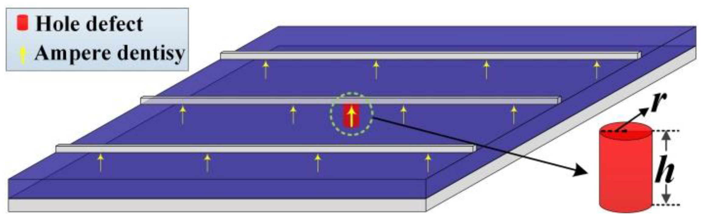
When the solar cell operates under reverse bias (where Vrev denotes the reverse-bias voltage) and the photogenerated carrier distribution matches the reverse-bias injected carrier distribution (as indicated by the yellow arrow in Figure 2), severe ohmic shunting due to resistive defects can occur.
The presence of low-resistance defects produces a strong ohmic shunt in the solar cell, resulting in significant Joule heating that can be described by the volumetric heat-source expression shown in Equation (6):
R hole = h σ hole π r 2 Q = Q H = V rev 2 R hole
where Rhole is the resistance of the columnar low-resistance defect, h is the column height, σhole denotes the electrical conductivity of the low-resistance region, r is the column radius, and Vrev is the reverse-bias voltage. The electrical conductivity of a well-performing silicon substrate is approximately 1 × 10⁻³ S/m [27]. In contrast, low-resistance defects formed by abnormal doping concentrations can electrically connect the front and rear electrodes of the solar cell, resulting in a much higher local conductivity, typically ranging from 1 to 102 S/m [28].
Table 5 illustrates the calculation of an equivalent volumetric heat source for a low-resistance defect based on Equation (6). In this analysis, the influence of the electric field distribution is neglected. Moreover, the metal contacts of the solar cell are assumed to be ideal, such that Joule heat losses at the contacts are negligible. Joule heat generation in regions without low-resistance defects is assumed to be uniformly distributed and is therefore not considered.

2.2.2. Silicon-Based Deep Scratch Defect Modeling

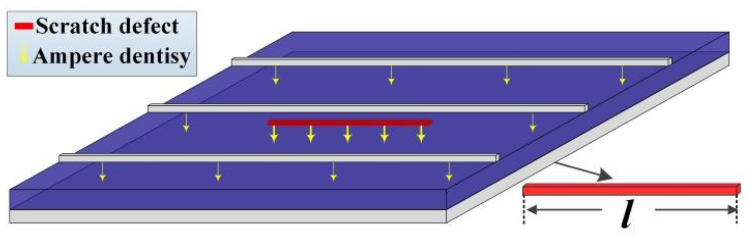
When deep scratches are present in the silicon substrate, a high recombination center can form in the emitter layer, leading to a sharp increase in current density in the scratched region [29], as indicated by the yellow arrow in Figure 3. Accordingly, a linear equivalent volumetric heat-source model is adopted, as illustrated in Figure 3.
Table 6 shows the energy distribution of the ideal single junction solar cell with a band gap of Eg = 1.11 eV [30].
Q0 denotes the intrinsic loss, QT is the thermalization heat loss, QJ represents the ohmic heat loss, POUT is the electrical power output of the solar cell, and QL is the equivalent loss associated with defects. Therefore, the equivalent heat source Q resulting from shunt formation induced by deep scratch defects is given in Equation (7):
Q = Q L = Q S Q 0 P OUT Q T Q J
When no anomalous shunt is present in the solar cell, the equivalent volumetric heat source satisfies QL = 0, as shown in Table 6. When a deep scratch in the silicon substrate induces power loss, a portion of the energy is converted into localized heat dissipation in the scratched region, resulting in the formation of a volumetric heat source with QL ≠ 0.

2.2.3. Simulation Setup and Numerical Modeling Results

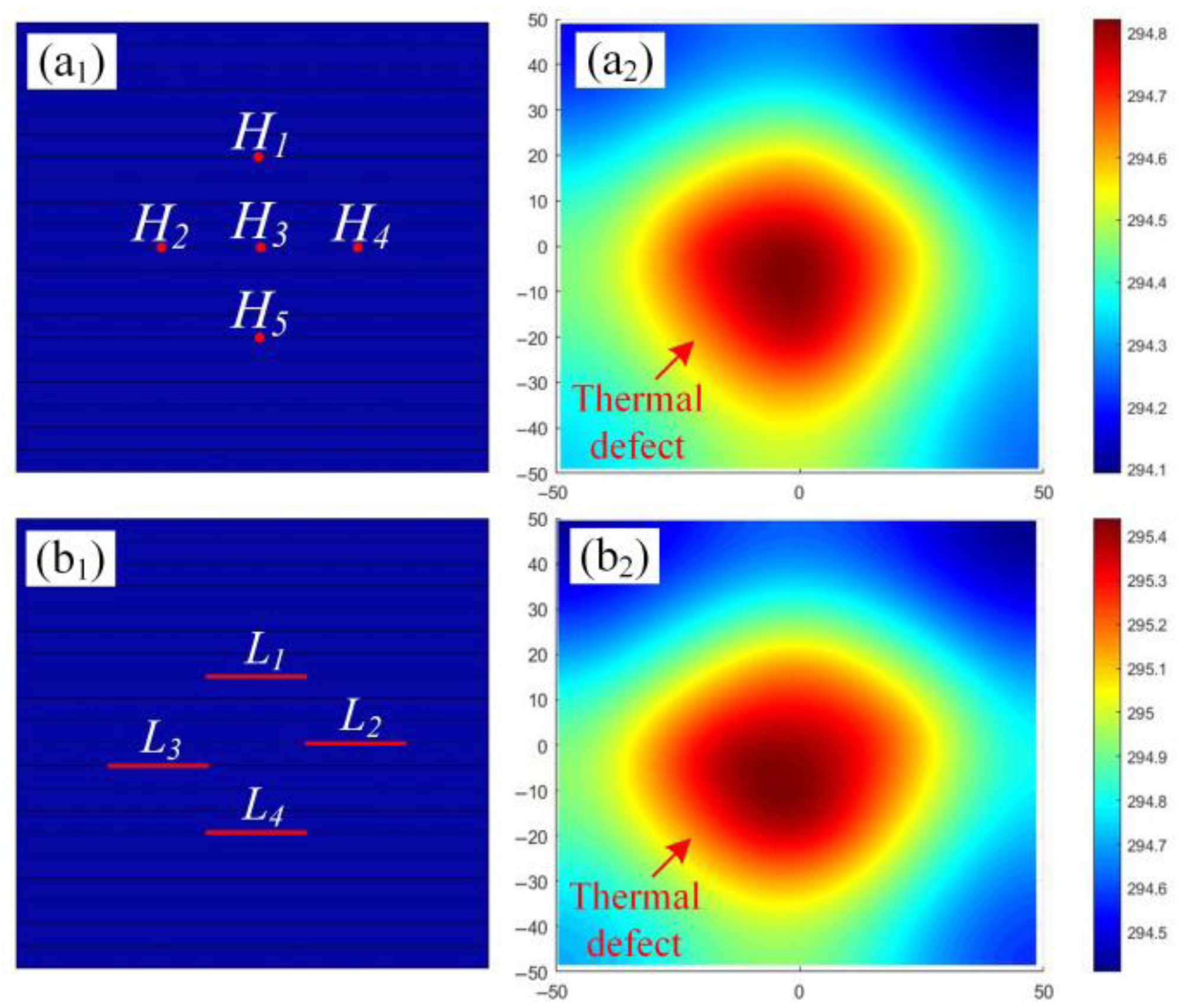
The above analysis provides the basis for defining equivalent volumetric heat sources associated with deep scratch and low-resistance defects in silicon-based solar cells. In the following section, an equivalent simulation model incorporating multiple volumetric heat sources is developed, and the resulting thermal distribution in the solar cell induced by different types of volumetric heat sources is analyzed in detail. Table 7 lists the locations and dimensions of the prescribed volumetric heat sources. The lengths of all linear heat sources are set to 20 mm, providing the necessary geometric parameters for subsequent simulations.
The simulation results containing prefabricated thermal defects are shown in Figure 4. Comparison of Figure 4a2,b2 shows that PV cell units containing different defective heat sources cannot directly distinguish the positional distribution of the internal volumetric heat sources through the distribution of the surface temperature, and it is more difficult to carry out a quantitative analysis of the internal thermal defects.

2.2.4. Experimental Validation of Low-Resistance Defect Model

To verify the accuracy of the finite element model for the equivalent heat source of the solar cell, experimental validation was conducted. The validation experiments were performed on a bare solar cell rather than a fully packaged module. This choice was made to reduce the influence of encapsulation layers and to enable a clearer assessment of the thermal response associated with defect-related heat sources, thereby facilitating validation of the underlying physical model.
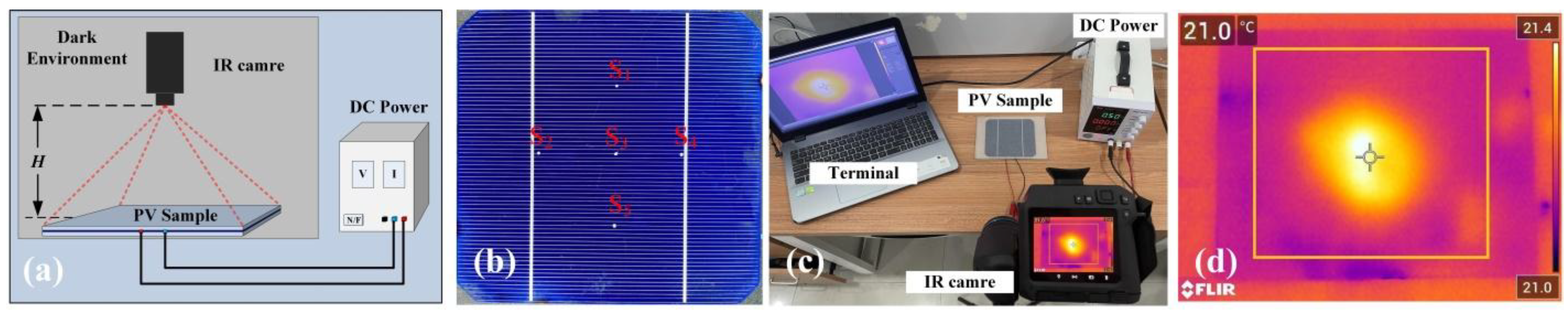
The basic configuration of the experimental platform for the differential method is shown in Figure 5a. In the experiment, a DC power supply (MS1510D Mastech Group, Shenzhen, China) was used to apply a stable reverse-bias voltage of 0.5 V to the solar cell. The cell was continuously energized for at least 1 min in a dark environment to stabilize its thermal and electrical properties (dark reverse-bias condition). A FLIR T1050sc(Teledyne FLIR, Wilsonville, OR, USA) infrared camera (thermal sensitivity < 20 mK and spatial resolution of 960 × 1280 pixels) was employed to record the temperature distribution of the solar cell samples. Before each measurement, the solar cell was allowed to cool naturally to room temperature to ensure measurement repeatability and accuracy. In the experimental samples, five artificial low-resistance defects with different sizes were fabricated by drilling holes in localized regions of the solar cell to create low-resistance shunting paths. The corresponding solar cell samples were denoted as S1–S5. In addition, the experimental procedure was repeated several times under identical conditions to minimize uncertainties arising from environmental and human factors. The recorded temperature profiles covered the entire surface of the solar cell.
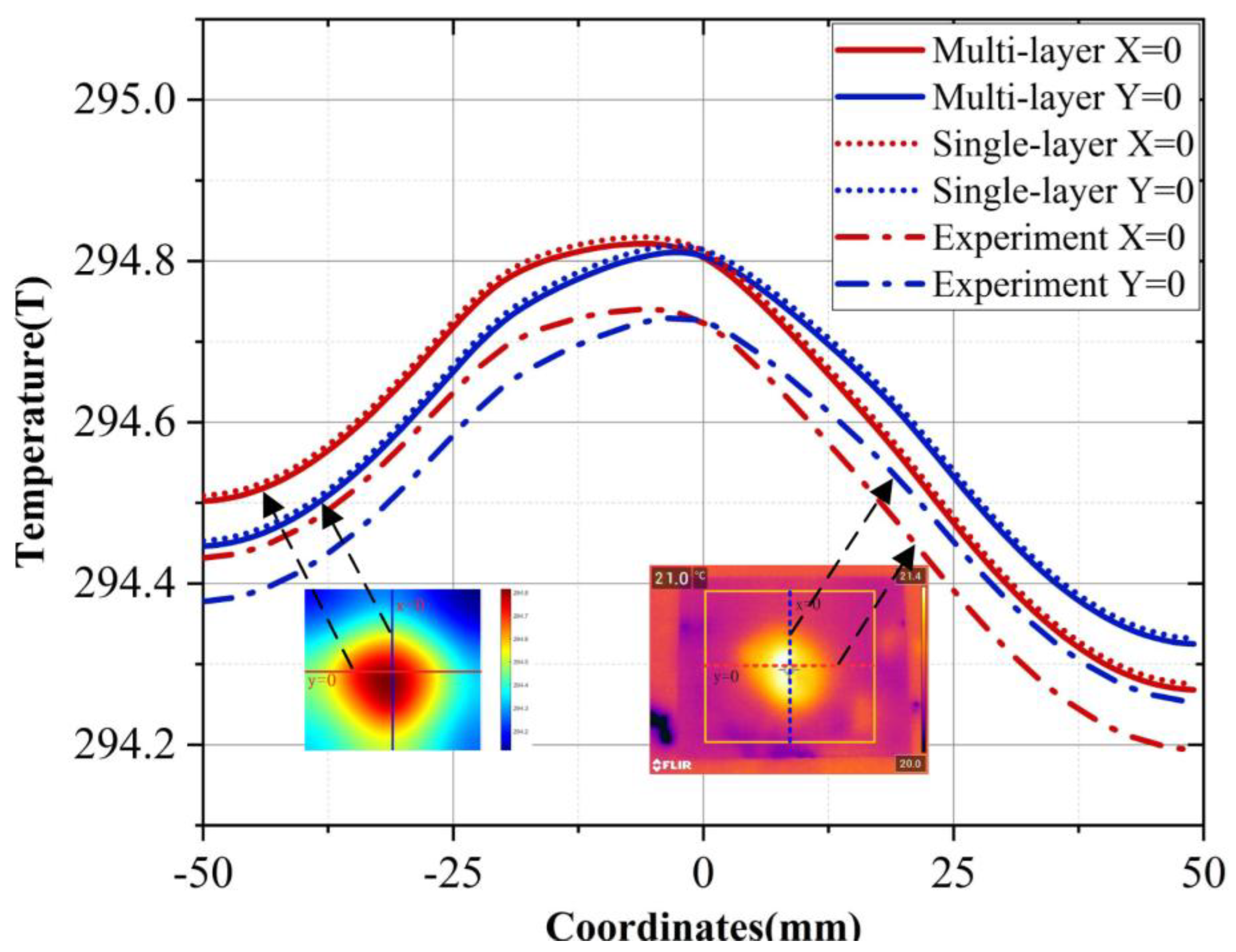
The solar cell sample containing low-resistance defects is shown in Figure 5b. The settings of the low-resistance defect parameters are consistent with those shown in Figure 4. The optical image of the experiment is shown in Figure 5c, while the corresponding infrared image acquired by the IR camera is shown in Figure 5d. A comparative analysis of the infrared measurement results and the simulation results is presented in Figure 6. Comparison of the surface temperature profiles obtained from the simulation model and the experimental samples reveals certain discrepancies. These differences are primarily attributed to imperfect thermal insulation between the experimental samples and the surrounding environment.

2.3. Methodology and Theoretical Analysis

2.3.1. Equivalent Single-Layer Thermal Conduction Theory

The previous section described that the solar cell consists of multiple layers made of different materials. According to Fourier’s law of heat conduction, the thermal conductivities of the individual layers, denoted by λ, can be equivalently represented by an effective thermal conductivity λ3 of a single layer. Based on this equivalence, the solar cell can be simplified into a single-layer heat-transfer model, and a differential model describing the surface temperature distribution induced by thermal defects within the equivalent layer can be established. As shown in Figure 7, according to Fourier’s law of heat conduction, the heat flux per unit area through a flat wall is given by:
q = t 1 t 2 L a / λ 1 = t 2 t 3 L b / λ 2
q = λ 3 t 4 t 5 L c
In the above expression, q denotes the heat flux through a flat wall per unit area. The temperatures t1, t2, t3, t4, and t5 represent the boundary temperatures of each layer, while λ1, λ2, and λ3 are the thermal conductivity coefficients of the corresponding materials. Letting λ 3 = L c L a λ 1 + L b λ 2 the following expression can be obtained:
q = λ 0 t 1 t 3 L 0
By comparing the above expressions, the heat flux per unit area in the model can be derived, allowing the multilayer structure to be simplified into an equivalent single-layer model. Thermal defects occur mainly in the silicon substrate layer. Moreover, heat-wave penetration into the overlying glass and EVA layers is negligible due to the much smaller grid-line scale. Therefore, a single-layer medium simplification can be adopted. In this approach, the two upper layers are treated as a single medium characterized by an equivalent thermal conductivity. Using Figure 7 together with Equations (7)–(9), the equivalent thermal conductivity of the single-layer medium is calculated. The comparison results, shown in Figure 6, indicate that the five heat sources are located at identical positions in both the multilayer model and the simplified single-layer model.
The relative error between the surface temperatures obtained from the single-layer and multilayer models ranges from approximately 1% to 3%. This range can be regarded as a practical limit of temperature mismatch between different material-layer models, because the multilayer structure cannot achieve the same ideal meshing quality as the single-layer model during mesh discretization. As a result, deviations in heat-flux propagation are inevitable.
In theory, if the mesh is refined to an ideal state, the surface temperature distributions of the single-layer and multilayer models should be fully consistent. Considering the observed relative error, the mesh was further refined, yielding more accurate results, as shown in Figure 6. These results verify the feasibility of the single-layer medium equivalence assumption.

2.3.2. Squared Even-Order Derivative Methodology

The principle of the SEOD method proposed in this paper is described below. First, Equation (11) presents the general heat conduction equation for a solid. Under steady-state conditions, the transient term vanishes; therefore, the heat conduction equation for a solid containing a heat source can be written as:
( λ T ) = Q
When a heat source exists within an object, the surface temperature T(x, y) in the direction perpendicular to the heat source varies with both the intensity and the spatial location of the heat source. This relationship can be expressed by the following equation:
T ( x , y ) = Q 4 π λ h 2 + x 2 + y 2
The parameter h represents the vertical separation between the internal heat source and the surface of the target object. The interdependence among T, Q, and h is governed by the previously established equation. Nevertheless, inferring thermal defect parameters-specifically the heat-source intensity Q and the depth h-is challenging when only the surface temperature field T is available. To overcome this limitation, the SEOD approach is introduced to enhance spatial resolution and thereby improve the estimation accuracy of defect-related thermal parameters. To further examine the differential behavior of defect-induced surface temperature variations, successive derivatives of the function F(x) with respect to x are calculated. The second-, fourth-, and sixth-order derivatives are selected for detailed analysis.
f ( x , y ) = ( T ( x , y ) ) 2 = Q 4 π λ 2 1 h 2 + x 2 + y 2
f 2 ( x , y ) = 2 f ( x , y ) x 2 2 + 2 f ( x , y ) y 2 2 f 4 ( x , y ) = 4 f ( x , y ) x 4 2 + 4 f ( x , y ) y 4 2 f 6 ( x , y ) = 6 f ( x , y ) x 6 2 + 6 f ( x , y ) y 6 2
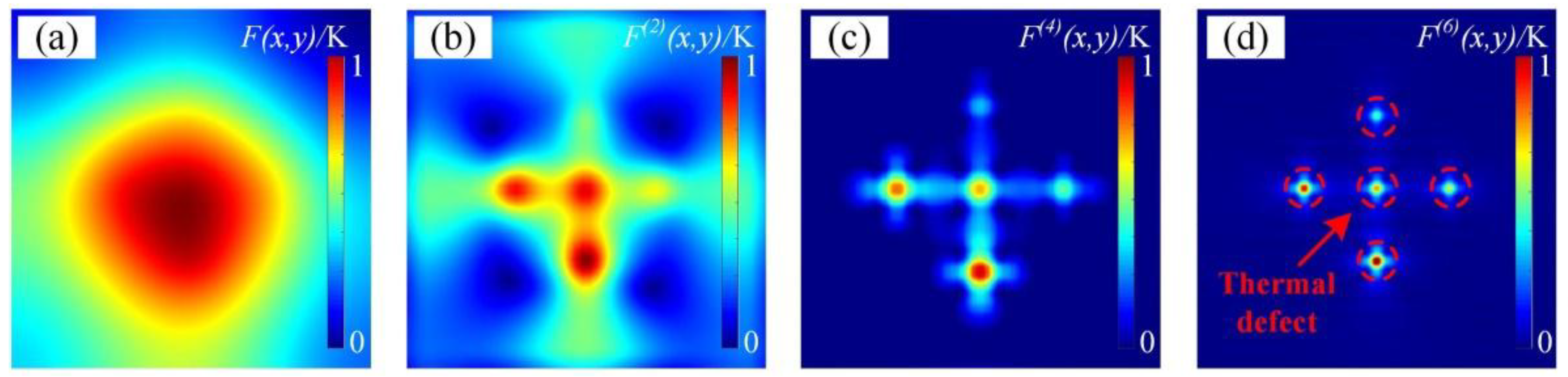
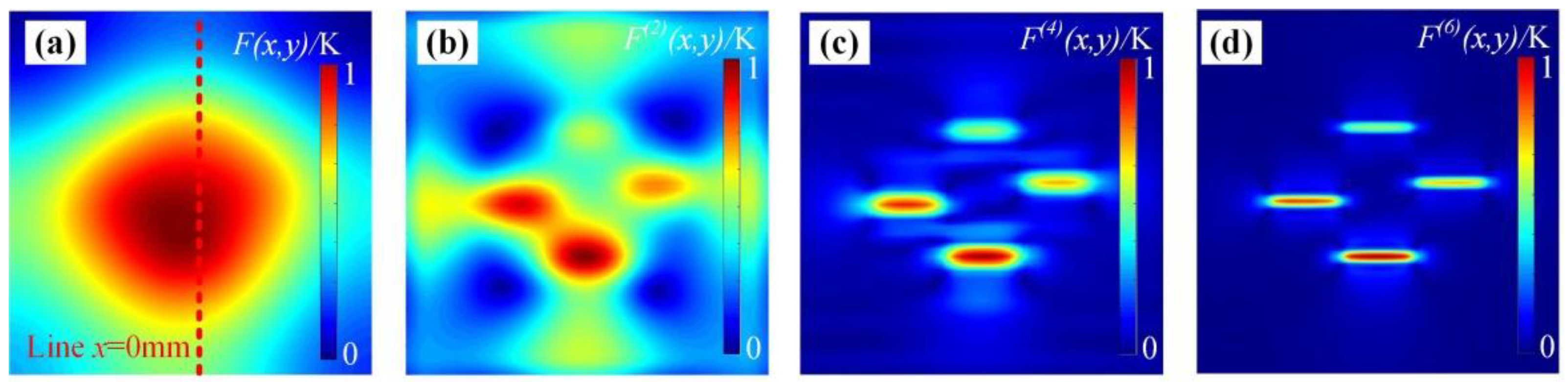
Figure 8 presents the temperature distribution map of a low-resistance defect together with the corresponding second-, fourth-, and sixth-order differential processing results. As illustrated in the figure, the unprocessed temperature distribution map exhibits only a smooth and gradually varying thermal profile, making it difficult to intuitively identify detailed information associated with internal heat-source defects. Although the thermal field generated by the defect is present, its manifestation on the surface is too subtle and spatially diffuse to enable clear localization when only the original temperature profile is considered.
However, after applying higher-order differential processing, the subtle temperature variations induced by the defect are significantly amplified, and the resulting derivative curves exhibit distinct peak features that correspond to the actual heat-source location. These peaks become progressively sharper and more easily distinguishable as the order of differentiation increases, thereby substantially improving the spatial resolution for defect identification. Consequently, the high-order differential results provide an intuitive and visually explicit indication of the defect position, thereby establishing a clearer foundation for the subsequent quantitative analysis presented in the following examples.

2.3.3. Quantitative Error Analysis of the SEOD Method

To further analyze the location and intensity of the internal heat source based on the surface temperature, the temperature profile along the y = 0 line is extracted and mathematically analyzed as follows:
F ( x ) = ( T ( x ) ) 2 = Q 4 π λ 2 1 h 2 + x 2
The second-, fourth-, and sixth-order derivatives of F(x) are calculated, respectively:
F ( 2 ) ( x ) = Q 2 8 π 2 λ 2 3 x 2 h 2 ( h 2 + x 2 ) 3 F ( 4 ) ( x ) = 3 Q 2 2 π 2 λ 2 h 4 10 x 2 h 2 + 5 x 4 ( h 2 + x 2 ) 5 F ( 6 ) ( x ) = 45 Q 2 π 2 λ 2 7 x 6 35 h 2 x 4 + 21 h 4 x 2 h 6 ( h 2 + x 2 ) 7
According to the properties of continuous functions, the derivative at an extremum is zero; therefore, the following equation is obtained:
F ( 3 ) ( L 2 ) = 3 Q 2 4 π 2 λ 2 L 2 h 2 L 2 2 h 2 + L 2 2 4 = 0 F ( 5 ) ( L 4 ) = 15 Q 2 2 π 2 λ 2 L 4 h 2 3 L 4 2 3 h 2 L 4 2 h 2 + L 4 2 6 = 0 F ( 7 ) ( L 6 ) = 56 Q 2 π 2 λ 2 L 6 ( L 6 h ) ( L 6 + h ) L 6 2 2 h L 6 h 2 L 6 2 + 2 h L 6 h 2 h 2 + L 6 2 8 = 0
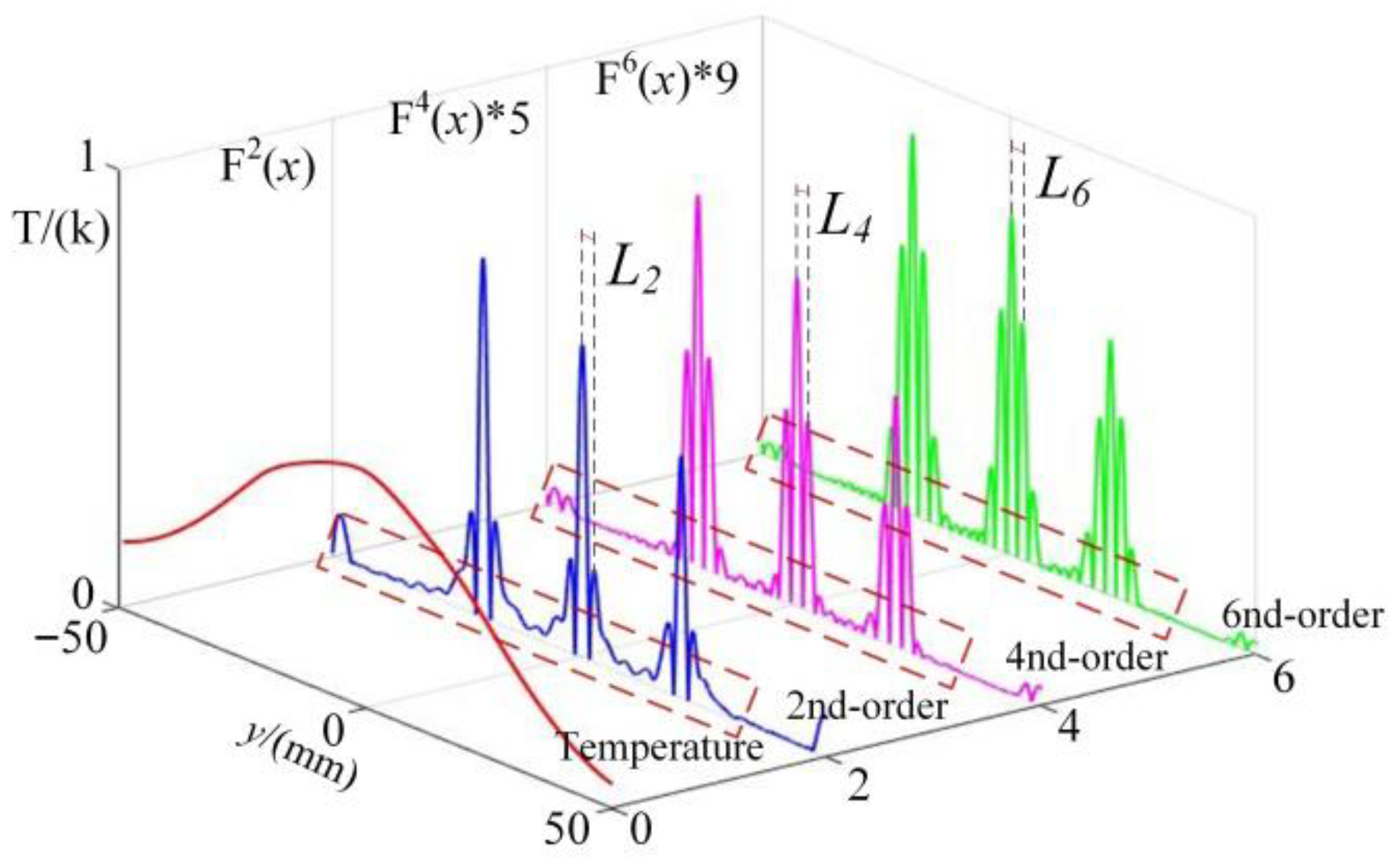
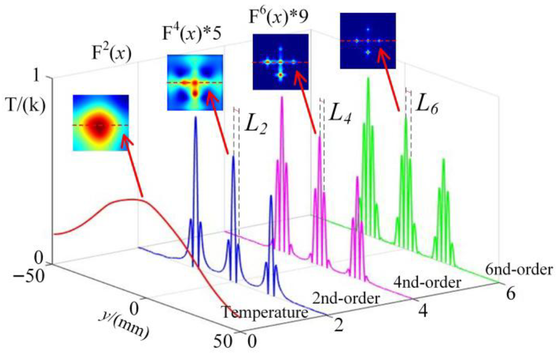
The parameters L2, L4, and L6 in the above equation are illustrated in Figure 9, where Q, L2, L4, and L6 are nonzero. Compared with the original temperature distribution curve, the corresponding differential curves exhibit distinct main and side peak features. A comparison of these graphical characteristics indicates that the widths of both the main peaks and the side peaks decrease as the differentiation order increases. In conjunction with Equation (17), the depth h can therefore be determined, as given in Equation (18).
h = L 2 h = 3 L 4 h = 1 3 2 3 / 2 L 6
Therefore, the proposed squared even-order derivative (SEOD) method can be used to determine the thermal defect depth h by analyzing surface temperature distribution characteristics based on the extremum features of the derived functions.
F ( 2 ) ( x = 0 ) = Q 2 8 π 2 λ 2 3 x 2 h 2 ( h 2 + x 2 ) 3 = | F 2 | F ( 4 ) ( x = 0 ) = 3 Q 2 2 π 2 λ 2 5 x 4 10 x 2 h 2 + h 4 ( h 2 + x 2 ) 5 = | F 4 | F ( 6 ) ( x = 0 ) = 45 Q 2 π 2 λ 2 7 x 6 35 h 2 x 4 + 21 h 4 x 2 h 6 ( h 2 + x 2 ) 7 = | F 6 |
The values of |F2|, |F4|, and |F6| in Equation (19) can be directly obtained from Figure 9. Combined with the defect depth h determined from Equation (18), the thermal defect strength Q can be further evaluated, as given in the following equation:
Q = 8 | F 2 π 2 λ 2 h 4 | Q = 2 3 | F 4 π 2 λ 2 h 6 | Q = 1 45 | F 6 π 2 λ 2 h 8 |
First, as shown in Figure 9, the unprocessed temperature curve does not clearly reveal information about the location or intensity of the internal heat source. Based on the second-order derivative results, the position of the main peak can be identified, which provides an initial estimate of the heat-source location through Equation (17). Subsequently, higher-order derivatives are employed to extract additional information related to the depth and precise location of the heat source. To further validate the feasibility of the proposed method, higher-order differentiation is applied to quantitatively determine the depth and location of the heat source.
To further verify the feasibility of the proposed method and assess the accuracy of the simulation results, the data presented in Figure 8 are subjected to a detailed quantitative analysis. Specifically, the equivalent single-layer model containing low-resistance thermal defects is investigated to determine both the spatial location and the intensity of the internal heat sources. By analyzing the surface temperature distribution and its corresponding squared even-order derivative responses, the capability of the proposed method in accurately localizing thermal defects and estimating their heat-source strength is systematically evaluated. Key characteristic parameters extracted from the derivative profiles are compared with the preset values in the simulation model to quantify the associated localization and intensity estimation errors. The resulting quantitative evaluation is summarized in Table 8, providing a clear validation of the effectiveness and reliability of the proposed approach.

3. Results and Discussion

3.1. Detection Results for Silicon-Based Deep Scratch Defects

In the previous section, the SEOD method was applied to the detection of low-resistance defect models, and the corresponding heat-source location and intensity were quantitatively analyzed. This section extends the analysis to the deep scratch defect model developed in Section 2. As shown in Figure 10, the surface infrared image of the deep scratch defect is similar to that of low-resistance defects, making it nearly impossible to directly identify the defect location from the raw IR image. Consequently, further quantitative characterization of the defect cannot be achieved using the original infrared data alone.
First, the original temperature data are smoothed and preprocessed using the Savitzky–Golay (S–G) filter. Subsequently, the second-, fourth-, and sixth-order differential result maps are calculated using the proposed method. The results indicate that, as the differentiation order of the SEOD method increases, the defect locations become progressively clearer and more distinguishable.

3.2. Quantitative Estimation of Defect Heat-Source Intensity

This study demonstrates that the proposed method can significantly enhance the spatial resolution for identifying heat-source defects. As the differential order in the SEOD method increases, the overlap between the surface temperature distribution and the defect location gradually decreases, thereby making the positional information of heat-source defects more distinct. Subsequently, the heat-source intensity of internal defects in the solar cell simulation model is determined by applying the approach introduced in Section 3. For the constructed low-resistance defective solar cell induced by a deep scratch, the surface temperature profile along x = 0 mm is extracted and subjected to higher-order differentiation, as illustrated in Figure 11. Based on this analysis, the total heat-source intensity of the defect is calculated using the second-, fourth-, and sixth-order derivatives, yielding values of QL1 = 0.108 W, QL4 = 0.251 W. These results reflect the operating state of the solar cell associated with thermal power dissipation induced by the defect.

3.3. Experimental Validation on PV Cell Samples

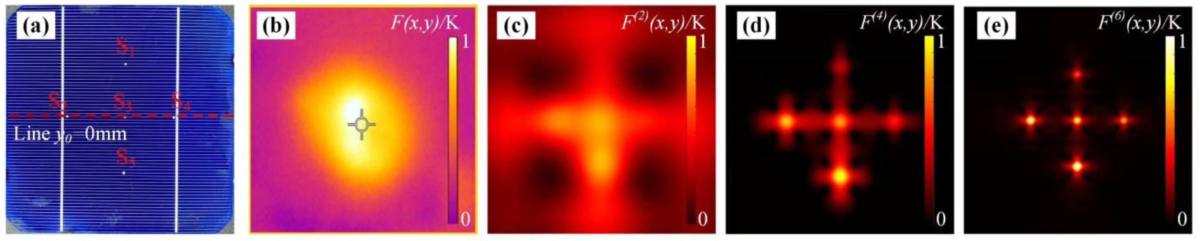
Figure 12 presents the surface temperature distributions of low-resistance defect samples together with the normalized results of second-, fourth-, and sixth-order differentiation, demonstrating that the SEOD method enables high-precision identification of thermal defects in real solar cell samples. As the derivative order increases, the contours of the thermal defects become progressively clearer. As shown in Figure 12c, second-order derivative processing enables coarse identification of severe thermal defects, whereas Figure 12e demonstrates that sixth-order derivative processing allows accurate localization of the defects.
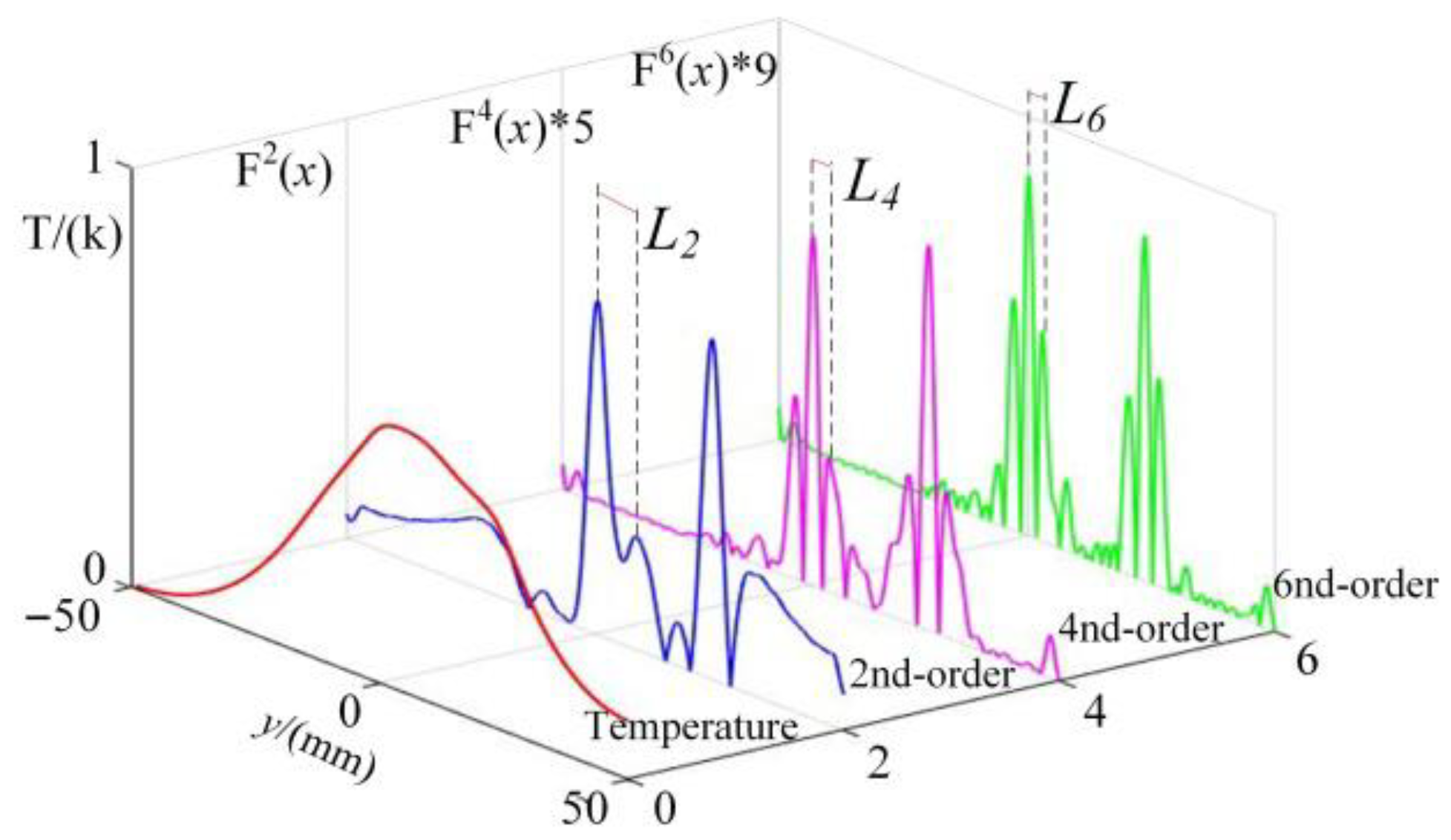
The surface temperature profile along y0 = 0 mm, extracted from Figure 12b, is subjected to higher-order differentiation, and the corresponding results are shown in Figure 13. A certain level of spurious signals appears in the higher-order differential curves due to limitations in experimental infrared data acquisition, as indicated by the red boxed region in Figure 13. However, this noise has a negligible influence on the principal side-lobe features of the differential curves. According to the SEOD method, three distinct thermal power losses are identified, with values of QS2 = 0.305 W, QS3 = 0.257 W, and QS4 = 0.204 W. These results are consistent with the preset low-resistance defect values of the experimental samples shown in Figure 12a, indicating that the proposed method is applicable to thermal defect detection in real operating solar cells and enables accurate quantitative analysis.
Based on the foregoing analysis, the validity and reliability of the proposed approach for identifying thermal anomalies in solar cells are preliminarily verified. The results further demonstrate that the method enables accurate quantitative characterization of thermal irregularities in solar cells under hotspot fault conditions. By enhancing the visual resolution of thermal faults and integrating quantitative hotspot detection, the proposed method enables accurate fault localization in solar cells. This overcomes the limitation of conventional infrared thermography, which cannot directly identify thermal defects, and provides a theoretical foundation for quantitative defect detection and health-state assessment of solar cells.
In the present study, experimental validation is limited to low-resistance defects under laboratory conditions, whereas silicon-based deep-scratch defects are investigated solely through numerical simulations. This is due to the difficulty of reproducibly introducing controlled scratches without compromising the structural integrity of the solar cell.
With respect to practical applications, the applicability and expected performance of the proposed SEOD method under real field conditions in photovoltaic power plants are further discussed. Considering typical on-site operating conditions such as environmental noise, natural convection, variations in radiative conditions, and uncertainties in infrared measurements, the proposed method is expected to maintain its capability for defect localization and quantitative characterization. This is achieved by suppressing slowly varying background temperature components and enhancing localized thermal anomaly responses through higher-order derivative feature extraction. Compared with conventional infrared thermography, which is more sensitive to global temperature fluctuations, the SEOD method emphasizes localized differential features and is therefore inherently more robust against slowly varying environmental disturbances commonly encountered during field inspections.

3.4. Uncertainty and Sensitivity Analysis

3.4.1. Uncertainty of Infrared Temperature Measurement

The experiments were conducted using a FLIR T1050sc (Teledyne FLIR, Wilsonville, OR, USA) infrared camera with a thermal sensitivity (NETD) better than 20 mK. Since multi-frame infrared sequences under identical operating conditions were not available, a conservative estimate of random temperature noise was performed based on the NETD specification combined with single-frame spatial statistics. Specifically, a background region of interest (ROI) with a relatively uniform temperature distribution was selected from the infrared image. The temperature data within this ROI were detrended, and the standard deviation of the residuals was then calculated to characterize the single-frame spatial noise level.
By combining the camera thermal sensitivity and the single-frame spatial noise estimate, the larger of the two values is adopted as the standard uncertainty of the random noise component. The quantifiable uncertainty budget of infrared temperature measurement under the present experimental conditions is summarized in Table 9. To avoid ambiguity with the symbols used for the Stefan–Boltzmann constant and electrical conductivity in the physical model, the symbol u is consistently used to denote standard uncertainty throughout the uncertainty analysis. The combined standard uncertainty of temperature measurement is uT = 0.525 K, which is subsequently propagated to the SEOD inversion results for uncertainty and sensitivity analyses.

3.4.2. Propagation of Temperature Measurement Uncertainty to SEOD Results

The SEOD method extracts defect information based on high-order spatial derivatives of the temperature field. While high-order differentiation enhances localized features, it also significantly amplifies temperature measurement noise. To evaluate the influence of temperature measurement uncertainty on the SEOD inversion results, a Monte Carlo approach was employed to perform uncertainty propagation analysis.
For a given noise standard uncertainty uT, random perturbations following a normal distribution were superimposed on the original temperature data. The complete processing chai-including filtering, derivative computation, and peak-feature extraction-was then repeatedly applied to each perturbed dataset. The dispersion of the SEOD main-peak localization results was then statistically evaluated over multiple realizations to quantify the uncertainty of the peak position. This approach avoids explicit analytical error propagation for the highly nonlinear inversion model and provides an intuitive assessment of the impact of temperature measurement noise on the SEOD inversion results.

3.4.3. Sensitivity Analysis of SEOD with Respect to Noise Level and Filtering Parameters

Based on the uncertainty propagation analysis of temperature measurements, the sensitivity of the SEOD method to noise level and filtering parameters was further investigated. Two commonly used preprocessing methods, namely Savitzky–Golay filtering and Gaussian filtering, were examined. Under different noise standard deviation levels, the stability of the second-, fourth-, and sixth-order derivative results was systematically evaluated.
Table 10 summarizes the statistical results of SEOD main-peak localization uncertainty under different noise levels, filtering methods, and derivative orders. The results indicate that, at low noise levels, lower-order derivatives maintain relatively high localization stability. As the noise level increases, the sensitivity of higher-order derivatives to noise becomes significantly enhanced, leading to a rapid increase in localization uncertainty. This behavior is particularly pronounced at the single-frame spatial noise level (uT = 0.525 K), indicating that high-order differentiation is more susceptible to noise interference under practical infrared measurement conditions.
In addition, the choice of filtering method also influences the stability of the SEOD method. Under the same noise conditions, an appropriate level of smoothing helps suppress high-frequency noise and improves the stability of lower-order derivatives, whereas excessive smoothing attenuates local features of the temperature field and consequently degrades the quantitative inversion of defect parameters. Therefore, a trade-off between noise suppression and feature preservation is required when selecting filtering parameters and derivative orders.

3.4.4. Relationship Between Uncertainty and Inversion Deviation

To further verify the relationship between uncertainty and inversion deviation, the SEOD-estimated source intensity was compared with the known reference values. Table 11 summarizes the deviations between the SEOD-inverted source intensity and the reference values for different derivative orders. The results indicate that, compared with the second-order derivative, higher-order derivatives can improve quantitative accuracy under low-noise conditions. However, in the presence of practical temperature measurement noise, their error growth trend is consistent with the sensitivity analysis discussed above.
In summary, infrared temperature measurement uncertainty and its amplification through high-order derivative operations constitute critical factors affecting the quantitative accuracy of SEOD inversion. Through uncertainty modeling, error propagation, and sensitivity analysis, a quantitative basis is provided for SEOD parameter selection and the assessment of result reliability.

4. Conclusions

A spatial-resolution and quantitative-assessment approach for identifying thermal defects in solar cells is presented in this study. The approach is constructed based on an even-order discretization scheme of the surface temperature distribution. Spatial localization and quantitative evaluation of thermal anomalies are achieved by analyzing critical parametric peak features extracted from higher-order temperature-gradient curves. The proposed framework is further applied to simulation models involving low-resistance defects and silicon-based deep scratches to substantiate its precision and practical applicability. In addition, strong detection performance is demonstrated when the approach is applied to experimental solar cell samples exhibiting low-resistance defects.
This strategy addresses key limitations of traditional infrared imaging by enabling clearer differentiation of defect-induced thermal responses and providing quantitative defect information. As a result, the method offers a reliable diagnostic pathway for defect detection throughout the entire lifecycle of solar cells, including manufacturing, transportation, installation, and long-term operation. The findings indicate that the proposed approach features lightweight computational requirements and high accuracy, thereby supporting future solar cell defect diagnostics and enhancing the operation and maintenance efficiency of photovoltaic power plants.

Author Contributions

Conceptualization, Z.D. (Zhizhen Du) and K.L.; methodology, Z.D. (Zhizhen Du); software, Z.D. (Zhizhen Du); formal analysis, Z.D. (Zhizhen Du); investigation, Z.D. (Zhizhen Du). and L.F.; data curation, Z.D. (Zhizhen Du); visualization, Z.D. (Zhizhen Du).; validation, K.L., Z.D. (Zhiqiang Dai). and G.W.; resources, K.L. and G.W.; writing—original draft preparation, Z.D. (Zhizhen Du); writing—review and editing, K.L. and G.W.; supervision, K.L.; project administration, K.L.; funding acquisition, K.L. and G.W. All authors have read and agreed to the published version of the manuscript.

Funding

This research was funded by the National Natural Science Foundation of China, grant number No. 52377161 and the National Key R&D Program of China, grant number No. 2022YFB4301202.

Data Availability Statement

The data supporting the findings of this study are available within the article. No additional datasets were generated or analyzed during the current study.

Conflicts of Interest

Author Zhiqiang Dai was employed by the State Grid Zhejiang Electric Power Company–Yiwu Power Supply Company. The remaining authors declare that the research was conducted in the absence of any commercial or financial relationships that could be construed as a potential conflict of interest.

References

  1. Sene, M.B.; Samoura, A.; Diouf, S.; Diao, A.; Mbow, C. Electrical modeling of a silicon photovoltaic solar cell: Comparative study of models characterizing the photovoltaic solar cell. Open J. Appl. Sci. 2023, 13, 1787–1795. [Google Scholar] [CrossRef]
  2. Gu, S.; Yuan, L.; Guo, K.; Huang, W.; Li, L.; Yang, Y.; Jiang, X.; Yuan, N.; Wang, Q.; Ding, J. Laser damage and post oxidation repair performance of n-TOPCon solar cells with laser assisted doping boron selective emitter. Sol. Energy Mater. Sol. Cells 2024, 274, 112988. [Google Scholar] [CrossRef] [Scilit]
  3. Lv, X.; Hu, Z.; Yang, L.; Huang, J.; Yu, X.; Jin, C.; Yang, D. Transmission electron microscopy study on the laser-cutting induced microdefects in silicon heterojunction solar cells. Sol. Energy Mater. Sol. Cells 2025, 292, 113792. [Google Scholar] [CrossRef] [Scilit]
  4. Tepner, S.; Lorenz, A. Printing technologies for silicon solar cell metallization: A comprehensive review. Prog. Photovolt. Res. Appl. 2023, 31, 557–590. [Google Scholar] [CrossRef] [Scilit]
  5. Dhimish, M.; Hu, Y. Rapid testing on the effect of cracks on solar cells output power performance and thermal operation. Sci. Rep. 2022, 12, 12168. [Google Scholar] [CrossRef] [Scilit]
  6. Kumar, R.; Puranik, V.E.; Gupta, R. Application of electroluminescence imaging to distinguish ohmic and non-ohmic shunting in inaccessible cells within a PV module. IEEE J. Photovolt. 2024, 14, 296–304. [Google Scholar] [CrossRef] [Scilit]
  7. Dhimish, M.; Theristis, M.; d’Alessandro, V. Photovoltaic hotspots: A mitigation technique and its thermal cycle. Optik 2024, 300, 171627. [Google Scholar] [CrossRef] [Scilit]
  8. Aghaei, M.; Fairbrother, A.; Gok, A.; Ahmad, S.; Kazim, S.; Lobato, K.; Oreski, G.; Reinders, A.H.M.E.; Schmitz, J.; Theelen, M.; et al. Review of degradation and failure phenomena in photovoltaic modules. Renew. Sustain. Energy Rev. 2022, 159, 112160. [Google Scholar] [CrossRef] [Scilit]
  9. Johnson, S.; Morales, D.; Fremouw, K.; Gould, I.E.; Borsa, T.; Johnston, S.; Palmstrom, A.; DeCrescent, R.A.; McGehee, M.D. How non-ohmic contact-layer diodes in perovskite pinholes affect abrupt low-voltage reverse-bias breakdown and destruction of solar cells. Joule 2025, 9, 102102. [Google Scholar] [CrossRef] [Scilit]
  10. Vaas, T.S.; Pieters, B.E.; Gerber, A.; Rau, U. Thermal stimulation of reverse breakdown in CIGS solar cells. IEEE J. Photovolt. 2023, 13, 398–403. [Google Scholar] [CrossRef] [Scilit]
  11. Lillo-Sánchez, L.; López-Lara, G.; Vera-Medina, J.; Pérez-Aparicio, E.; Lillo-Bravo, I. Degradation analysis of photovoltaic modules after operating for 22 years. A case study with comparisons. Sol. Energy 2021, 222, 84–94. [Google Scholar] [CrossRef] [Scilit]
  12. Da Silva, E.G.; Franchi, C.M.; Treter, M.E.; Gamarra, D.F.T. Fault detection in photovoltaic modules using I–V curves and machine learning. Evol. Intell. 2025, 18, 100. [Google Scholar] [CrossRef] [Scilit]
  13. Akram, M.W.; Bai, J.; Xuan, C.; Xiaotuo, X.; Hu, J.; Wu, S. Advancing photovoltaic cells defect detection in electroluminescence images through exploring multiple object detectors. Sol. Energy Mater. Sol. Cells 2025, 292, 113777. [Google Scholar] [CrossRef] [Scilit]
  14. Kumar, S.; Jena, P.; Sinha, A.; Gupta, R. Application of infrared thermography for non-destructive inspection of solar photovoltaic module. J. Non Destr. Test. Eval. 2017, 6, 25–32. [Google Scholar]
  15. Ali, M.U.; Khan, H.F.; Masud, M.; Kallu, K.D.; Zafar, A. A machine learning framework to identify the hotspot in photovoltaic module using infrared thermography. Sol. Energy 2020, 208, 643–651. [Google Scholar] [CrossRef] [Scilit]
  16. Haidari, P.; Hajiahmad, A.; Jafari, A.; Nasiri, A. Deep learning-based model for fault classification in solar modules using infrared images. Sustain. Energy Technol. Assess. 2022, 52, 102110. [Google Scholar] [CrossRef] [Scilit]
  17. Tsanakas, J.A.; Chrysostomou, D.; Botsaris, P.N.; Gasteratos, A. Fault diagnosis of photovoltaic modules through image processing and Canny edge detection on field thermographic measurements. Int. J. Sustain. Energy 2015, 34, 351–372. [Google Scholar] [CrossRef] [Scilit]
  18. Bu, C.; Shen, R.; Bai, W.; Chen, P.; Li, R.; Zhou, R.; Li, J.; Tang, Q. CNN-based defect detection and classification of PV cells by infrared thermography method. Nondestruct. Test. Eval. 2025, 40, 1752–1769. [Google Scholar] [CrossRef] [Scilit]
  19. He, Y.; Du, B.; Huang, S. Noncontact electromagnetic induction excited infrared thermography for photovoltaic cells and modules inspection. IEEE Trans. Ind. Inform. 2018, 14, 5585–5593. [Google Scholar] [CrossRef] [Scilit]
  20. Asadpour, R.; Sulas-Kern, D.B.; Johnston, S.; Meydbray, J.; Alam, M.A. Dark lock-in thermography identifies solder bond failure as the root cause of series resistance increase in fielded solar modules. IEEE J. Photovolt. 2020, 10, 1409–1416. [Google Scholar] [CrossRef] [Scilit]
  21. Breitenstein, O.; Rakotoniaina, J.P.; Schmidt, J. Comparison of shunt imaging by liquid crystal sheets and lock-in thermography. In Proceedings of the 12th Workshop on Crystalline Solar Cell Materials and Processes, Breckenridge, CO, USA, 11–14 August 2002; Volume 12, pp. 244–247. [Google Scholar]
  22. Litvinenko, S.; Ilchenko, L.; Kaminski, A.; Kolenov, S.; Laugier, A.; Smirnov, E.; Strikha, V.; Skryshevsky, V. Investigation of the solar cell emitter quality by LBIC-like image techniques. Mater. Sci. Eng. B 2000, 71, 238–243. [Google Scholar] [CrossRef] [Scilit]
  23. Salazar, A.M.; Macabebe, E.Q.B. Hotspots detection in photovoltaic modules using infrared thermography[C]//MATEC web of conferences. EDP Sci. 2016, 70, 10015. [Google Scholar]
  24. Cardinale-Villalobos, L.; Meza, C.; Méndez-Porras, A.; Murillo-Soto, L.D. Quantitative comparison of infrared thermography, visual inspection, and electrical analysis techniques on photovoltaic modules: A case study. Energies 2022, 15, 1841. [Google Scholar] [CrossRef] [Scilit]
  25. Dallaev, R.; Pisarenko, T.; Papež, N.; Holcman, V. Overview of the current state of flexible solar panels and photovoltaic materials. Materials 2023, 16, 5839. [Google Scholar] [CrossRef] [Scilit]
  26. Sun, V.; Asanakham, A.; Deethayat, T.; Kiatsiriroat, T. A new method for evaluating nominal operating cell temperature (NOCT) of unglazed photovoltaic thermal module. Energy Rep. 2020, 6, 1029–1042. [Google Scholar] [CrossRef] [Scilit]
  27. Vergura, S.; Acciani, G.; Falcone, O. A finite-element approach to analyze the thermal effect of defects on silicon-based PV cells. IEEE Trans. Ind. Electron. 2011, 59, 3860–3867. [Google Scholar] [CrossRef] [Scilit]
  28. Roy, S.; Gupta, R. Quantitative estimation of shunt resistance in crystalline silicon photovoltaic modules by electroluminescence imaging. IEEE J. Photovolt. 2019, 9, 1741–1747. [Google Scholar] [CrossRef] [Scilit]
  29. Breitenstein, O.; Rakotoniaina, J.P.; Al Rifai, M.H.; Werner, M. Shunt types in crystalline silicon solar cells. Prog. Photovolt. Res. Appl. 2004, 12, 529–538. [Google Scholar]
  30. Hirst, L.C.; Ekins-Daukes, N.J. Fundamental losses in solar cells. Prog. Photovolt. Res. Appl. 2011, 19, 286–293. [Google Scholar] [CrossRef] [Scilit]
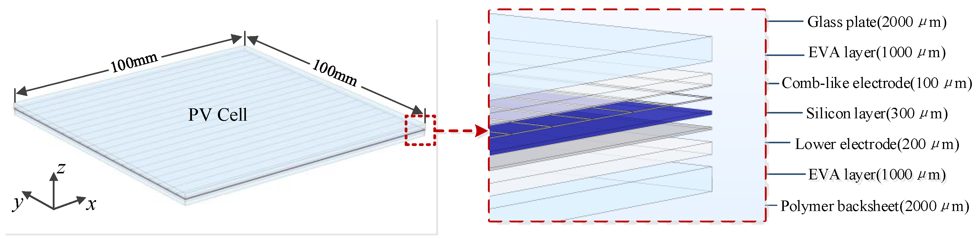
Figure 1. 3D model of a PV cell with protective layers (Colors are used to distinguish different layers).
Inventions 11 00014 g001
Figure 2. Low-resistance defect equivalent volume heat source diagram.
Inventions 11 00014 g002
Figure 3. Silicon-based deep scratch equivalent volume heat source diagram.
Inventions 11 00014 g003
Figure 4. Schematic diagram of precast thermal defect location (a1) low-resistance defect (b1) silicon based deep scratch; surface temperature distribution of defect simulation model (a2) low-resistance defect (b2) silicon based deep scratch. (H1–H5 and L1–L4 indicate heat sources with increasing power levels).
Inventions 11 00014 g004
Figure 5. PV cell infrared image experiment platform and introduction of experimental platform.((a) Schematic diagram of the infrared imaging experimental setup. (b) PV cell sample with artificial low-resistance defects (S1–S5). (c) Photograph of the experimental platform. (d) Infrared thermal image of the PV cell during operation.).
Inventions 11 00014 g005
Figure 6. Comparison of surface transversal temperature between simulation and experiment.
Inventions 11 00014 g006
Figure 7. Multilayer media equivalent model.
Inventions 11 00014 g007
Figure 8. Analysis outputs of the single-layer simulation model: (a) surface temperature distribution, (b) result of the second-order derivative, (c) result of the fourth-order derivative, and (d) result of the sixth-order derivative.
Inventions 11 00014 g008
Figure 9. Extraction of principal side peak characteristics of surface transversal D of a single layer simulation model.
Inventions 11 00014 g009
Figure 10. The original infrared image of simulation model and the result of differential processing. (a) Original infrared image, (b) Second-order derivative, (c) Fourth-order derivative, (d) Sixth-order derivative.
Inventions 11 00014 g010
Figure 11. Higher-order derivative characteristics extracted at x = 0.
Inventions 11 00014 g011
Figure 12. Normalized-amplitude analysis for the experimental scenario: (a) defect-containing sample 2, (b) infrared reference image, (c) second-order differential imaging, (d) fourth-order differential imaging, and (e) sixth-order differential imaging.
Inventions 11 00014 g012
Figure 13. The derivative of a line y0 = 0 on an experimental sample.
Inventions 11 00014 g013
Table 1. Annual power generation and failure rate of PV cell plant [11].
LocationOperation PeriodSampleDefect in ModulePmax Total Degradation (%)
Seville (Spain)22 years56 PV modules
53 Wp, 36 cells.
Scratch: 89.29%
Hot spot: 3.57%
−30.9%
Porto Alegre (Brazil)15 years48 PV modules
100 Wp, 72 cells.
Scratch: 27%−11.5%
Malaga (Spain)12 years42 PV modules
53 Wp, 36 cells.
Scratch: 60%
Hot spot: 7%
−9.5%
Table 2. Thermal parameter of each layer.
MaterialGlassEVAAgSiPolymer Backsheet
λ [W/(m·K)]1.090.154301450.23
ρ [kg/m3]250094810,50023201180
CP [J/(kg·K)]75021002357031250
Table 3. Heat convection parameter.
Nuλa (W/(m·K))L (mm)Tamb (K)
550.025100293.15
Table 4. Interlayer material emissivity.
MaterialGlassEVAAgSiPolymer Backsheet
ε0.90.90.10.850.9
Table 5. Equivalent volumetric heat source with low-resistance defect in reverse bias state.
Vrev (v)σhole (S/m)r (mm)h (mm)
0.51020.10.3
Table 6. Solar band gap Eg = 1.11 eV incident energy distribution in ideal monocrystalline silicon (incident solar energy = 1000 W/m2).
Solar EnergyIntrinsic LossVariable Loss
QSQ0QTQJPOUT
1.8 W
10 W3.2 W3.75 W1.25 W
Table 7. Multi-thermal defect model simulation results.
Defect12345
QH (W)0.150.300.250.200.35
PH (x, y)0, 20−20, 00, 020, 00, −20
QL (W)0.10.150.20.25
PL (x, y)0, 1520, 0−20,−50, −20
Table 8. Error analysis of thermal defect information in single layer simulation model.
DefectsH1H2H3H4H5
ActualPosition (mm)0, 20−20, 00, 020, 00, −20
Intensity (W)0.150.300.250.200.35
SecondPosition (mm)0, 19.8−20.2, −0.3−0.3, −0.319.8, −0.2−0.1, −20.1
Error (mm)0, 0.20.2, 0.30.3, 0.30.2, 0.20.1, 0.1
Intensity (W)0.1690.3420.2890.2300.395
Error (%)11.212.313.513.011.4
FourthPosition (mm)0, 19.9−20.1, −0.2−0.2, −0.119.8, −0.1−0.1, −20
Error (mm)0, 0.10.1, 0.20.2, 0.10.2, 0.10.1, 0
Intensity (W)0.1600.3210.2700.2150.377
Error (%)6.256.547.406.987.16
SixthPosition (mm)0, 20−20, −0.1−0.1, −0.119.9, 00, −20
Error (mm)0, 00, 0.10.1, 0.10.1, 00, 0
Intensity (W)0.1560.3140.2620.2090.367
Error (%)3.854.464.584.304.63
Table 9. Uncertainty budget of infrared temperature measurement.
ComponentSymbolStandard Uncertainty (K)
Thermal sensitivity (NETD)uNETD0.02
Single-frame spatial noise (ROI-based)uspatial0.525
Random noise componenturand0.525
Combined temperature uncertaintyuT0.525
Table 10. Sensitivity of SEOD peak localization to noise level and filtering parameters.
Noise Standard Uncertainty uT (K)Filtering MethodDerivative OrderPeak Localization Uncertainty ux (Samples)
0.02S-G (W = 11, p = 3)2th2.66
0.02S-G (W = 11, p = 3)4th78.45
0.02S-G (W = 11, p = 3)6th81.14
0.02Gaussian (σg = 2)2th0.72
0.02Gaussian (σg = 2)4th57.17
0.02Gaussian (σg = 2)6th80.22
0.04S-G (W = 11, p = 3)2th6.56
0.04S-G (W = 11, p = 3)4th83.62
0.04S-G (W = 11, p = 3)6th85.31
0.1S-G (W = 11, p = 3)2th42.78
0.1S-G (W = 11, p = 3)4th85.87
0.1S-G (W = 11, p = 3)6th87.01
0.525S-G (W = 11, p = 3)2th82.36
0.525S-G (W = 11, p = 3)4th87.92
0.525S-G (W = 11, p = 3)6th88.65
Table 11. Deviation between SEOD-inverted and actual source intensity.
DefectActual Source Intensity Qactual (W)2th-Order SEOD (W)Error (%)4th-Order SEOD (W)Error (%)6th-Order SEOD (W)Error (%)
H10.150.16911.20.166.250.1563.85
H20.30.34212.30.3216.540.3144.46
H30.250.28913.50.277.40.2624.58
H40.20.23130.2156.980.2094.3
H50.350.39511.40.3777.160.3674.63
Disclaimer/Publisher’s Note: The statements, opinions and data contained in all publications are solely those of the individual author(s) and contributor(s) and not of MDPI and/or the editor(s). MDPI and/or the editor(s) disclaim responsibility for any injury to people or property resulting from any ideas, methods, instructions or products referred to in the content.