A Procedure for Performing Reproducibility Assessment of the Accuracy of Impact Area Classification for Structural Health Monitoring in Aerospace Structures ^†

Abstract

The principal objective of this work is to develop an optimized procedure that guarantees the reproducibility of results across different applications and laboratories, facilitating potential field applications of methodologies for Structural Health Monitoring in aerospace structures. The focus is to accurately detect and localize impact areas on planar structures using in situ transducers and Machine Learning (ML) techniques. The research concentrates on an aluminum plate where impacts are generated by metal spheres of different masses dropped from a fixed height. The resulting Lamb waves are detected by PZT sensors glued on the surface. Various data processing and feature extraction algorithms are implemented and compared to extract the differences in Time of Flight (ΔToF). The obtained features are used for training ML classification models. Then, the influence of various parameters in signal acquisition and data processing are assessed along with the reproducibility of the results. For this reason, an interlaboratory comparison is conducted in which the trained models are applied to data collected under varying conditions. The experimental results show that the most influencing factors for impact area classification are the algorithm for ΔToF estimation, the number of training points used in ML models, the type of classification model, the distribution of the impact points on the component, and their balance in the classification area. This evidence suggests approaches for reducing both issues, therefore improving the reproducibility of results.

1. Introduction

In the aerospace industry, ensuring structural integrity and early detection of defects is of paramount importance for several reasons. For example, structure monitoring improves safety, reduces unnecessary inspection and maintenance costs, and minimizes the weight of aircraft components during the design phase. To achieve these aims, non-destructive testing (NDT) techniques are commonly employed for structural assessments, often alongside theoretical models and simulations [1,2,3,4,5,6].

In recent decades, Structural Health Monitoring (SHM) has gained a lot of attention as its significance has become increasingly apparent. SHM involves a range of techniques that use sensor networks and sophisticated algorithms to provide real-time evaluations of structural reliability [7]. An SHM system is designed to detect structural damage in order to formulate a potential intervention plan. The damage identification process can be delineated into three primary stages: detection, diagnosis, and prognosis [8].

The first SHM phase is damage detection. This includes changes to the material and/or geometric properties of these structures which adversely affect the system’s performance [9].

Diagnosis is an ongoing process throughout the structure’s lifecycle. This stage aims to monitor its operational condition and identify any damage resulting from various factors such as material stress, collisions, or aging. This phase is further divided into passive and active diagnosis [10]. Passive diagnosis relies on sensors that capture any changes in the structure during normal use. In contrast, active diagnosis uses an actuator to apply stress, generating a response that is measured by receiving sensors, thus enabling assessment of the structure’s condition.

The prognosis phase focuses on assessing the severity of any identified damage and estimating the remaining lifespan of the structure.

One of the key concepts of SHM is online monitoring, allowing all of the previously described phases to be carried out in embedded systems. These “smart” structures overcome several problems of traditional inspection methods. In fact, manual inspections, NDT, and model-based techniques are often labor-intensive, time-consuming, and may be inadequate for detecting hidden or developing damage [11]. This approach has several potential benefits:

• Facilitates condition-based maintenance.
• Prevents catastrophic damage.
• Reduces machine downtime.
• Eliminates human error.
• Monitors inaccessible components.

In the aerospace sector, the integrity and longevity of structures are significantly influenced by the frequency and intensity of impacts from orbiting objects, space debris, or, for aircraft, bird strikes [12].

One subset of SHM methods used for examining the impacts of external objects on a thin planar plate uses a passive diagnosis system in conjunction with the analysis of Lamb waves. Lamb waves represent an acoustic emission (AE) phenomenon and are a combination of longitudinal and transverse modes. The propagation properties of these waves depend on the excitation source and the structural geometry. Another important aspect of Lamb waves is their dispersive behavior. This means that propagation speed is frequency-dependent. A significant advantage of these waves is their ability to travel over long distances, thereby eliminating the need to access the structure using local detection methods [1,13].

To identify the impact damage, several studies have used Machine Learning (ML) techniques applied on AE signals. In [14], the authors developed an SHM system that identifies the source of an AE, allowing them to study the A0 mode of Lamb waves in a composite structure using PZT (Pb[Zr_xTi_1−x]O₃) sensors. The signals are analyzed by means of Continuous Wavelet Transform (CWT) and then the impact coordinates are determined by solving a set of non-linear equations using a combination of a local Newton iterative method and global unconstrained optimization. Other impact point localization algorithms are presented in the literature [15,16]. These methods do not use ML techniques and focus on the use of analytical techniques like FEM models combined with specific experimental setups. In all of these cases, the authors use closed-form mathematical solutions. Other approaches used for localizing impacts take advantage of ML techniques, as in [17]. Here, the authors used pre-trained stacked autoencoders in a two-step approach that first localizes AE sources and then characterizes them. Another method is presented in [18] and is based on the time reversal technique and ML approaches. This algorithm consists of two steps: The first involves a training process, where a baseline of structural responses from impact tests is computed. The second step assesses the impact location by utilizing the highest cross-correlation coefficient, derived from interpolating the impact response baseline. Other approaches are based on different models, as presented in [19]. In that study, automatic impact detection and localization use Random Forest and Stacked Autoencoder (SAE) techniques. A steel ball is dropped on a composite aircraft elevator to collect AE signals. The Random Forest algorithm is trained on 3600 AE samples with 15 features to identify impact zones, while the SAE utilizes both raw AE signals and their fast Fourier Transform (FFT) for impact localization. All of these studies demonstrate the potential of applying signal processing and ML techniques in SHM based on AEs with reference to specific cases and applications. Nevertheless, an important requirement to be discussed concerns the reproducibility of each approach, as experimental methods must be able to achieve accurate results even when used in different situations. Accurate bias and uncertainty analysis mitigates the effect of systematic and random errors. It is essential to quantitively estimate those effects to support interlaboratory comparisons, which are useful for assessing the effects of the such improvements [20]. This is more relevant when ML methods are used.

Based on the above considerations, this paper aims to assess the effects of many aspects of the procedure, from the measurement phase to data processing, on the final reproducibility of the data, including a comparison of results with measurements carried out in different laboratories. This paper is an extension of a preliminary work presented by the authors at the IEEE MetroInd 2025 conference [21]. The present study aims to evaluate the accuracy of different methods that use ML algorithms for identifying the area of impact of metal spheres of different masses. These are dropped on the surface of an aluminum plate in different locations, therefore generating elastic waves that propagate through the component and are measured by Piezo Wafer Active sensors (PWASs). The feature of interest for impact localization is the difference between the Times of Flight (ΔToFs) of two vibration signals. The content presented in [21] is expanded here, as we assess the influence of different parameters on the variability of the results and the possible systematic effects that influence the localization capabilities and variability of the trained models. In particular, the aspects examined are the number of impact points of each area of interest, its layout, and the strategy for generating and analyzing the impacts. With reference to this, the parameters evaluated are the type and material of spheres, the number of repeated impacts on the same point used for building the training dataset for the ML models, the algorithm used for ΔToF evaluation, and the frequency of acquisition of the acoustic signal. Moreover, different classification algorithms are compared for localizing the impacts areas. To assess the reproducibility of the methods and results, an interlaboratory comparison is performed where the trained models are used on data acquired in different test and laboratory conditions.

In Section 2, the test bench and the data acquisition and processing techniques are described, highlighting the parameters that influence the variability of results, which are theoretically and experimentally analyzed. In Section 3, the results of the parametric analysis are described and discussed to evaluate the most important parameters to be kept under control. Finally, an interlaboratory comparison is presented to assess the reproducibility of the experimental information.

The final section of this paper presents the conclusions.

2. Materials and Methods

2.1. Experimental Setup and Measurement Chain

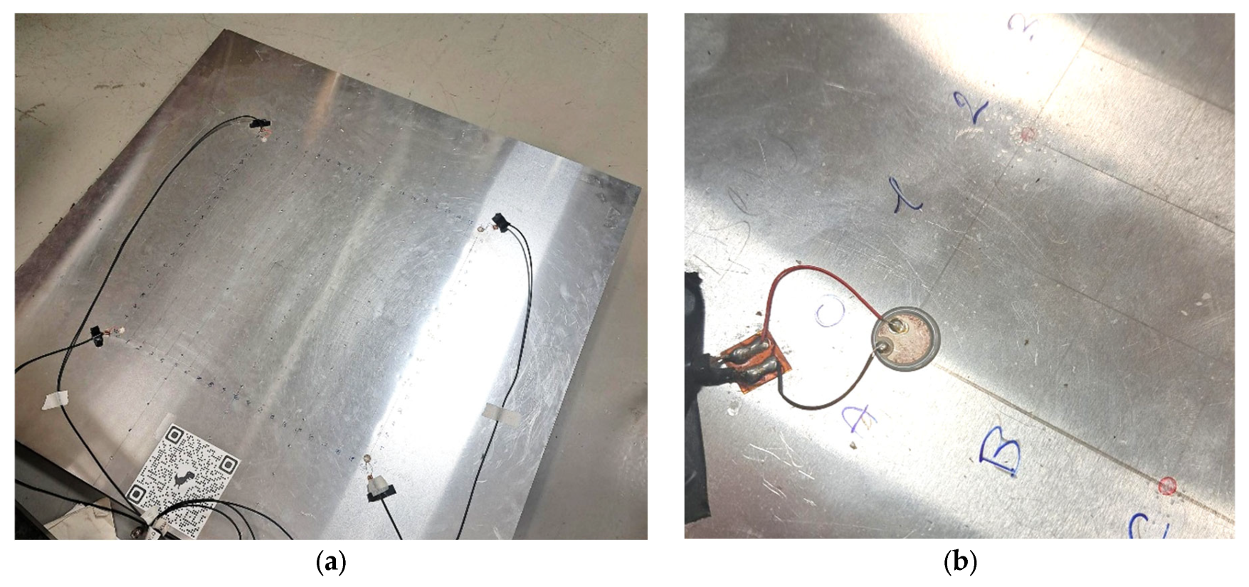
The experimental setup centers on an aluminum alloy plate, which is a component of a complex structure, such as fuselage skin or wing surfaces, in a real-world context. The experimental setup used in this work is presented in Figure 1.

As shown in Figure 1a, the aluminum alloy plate utilized in the experiment is representative of a portion of a panel used in the aerospace sector. It is 1000 mm in both length and width, with a thickness of 1.5 mm. It has an elastic modulus of 72 GPa, a Poisson’s ratio of 0.33, and a density of 2700 kg/m³. This plate is positioned on a foam rubber mattress that dampens its movements. This setup avoids unwanted vibrations and facilitates the detection of acoustic waves that propagate solely within the plate’s thickness as Lamb waves.

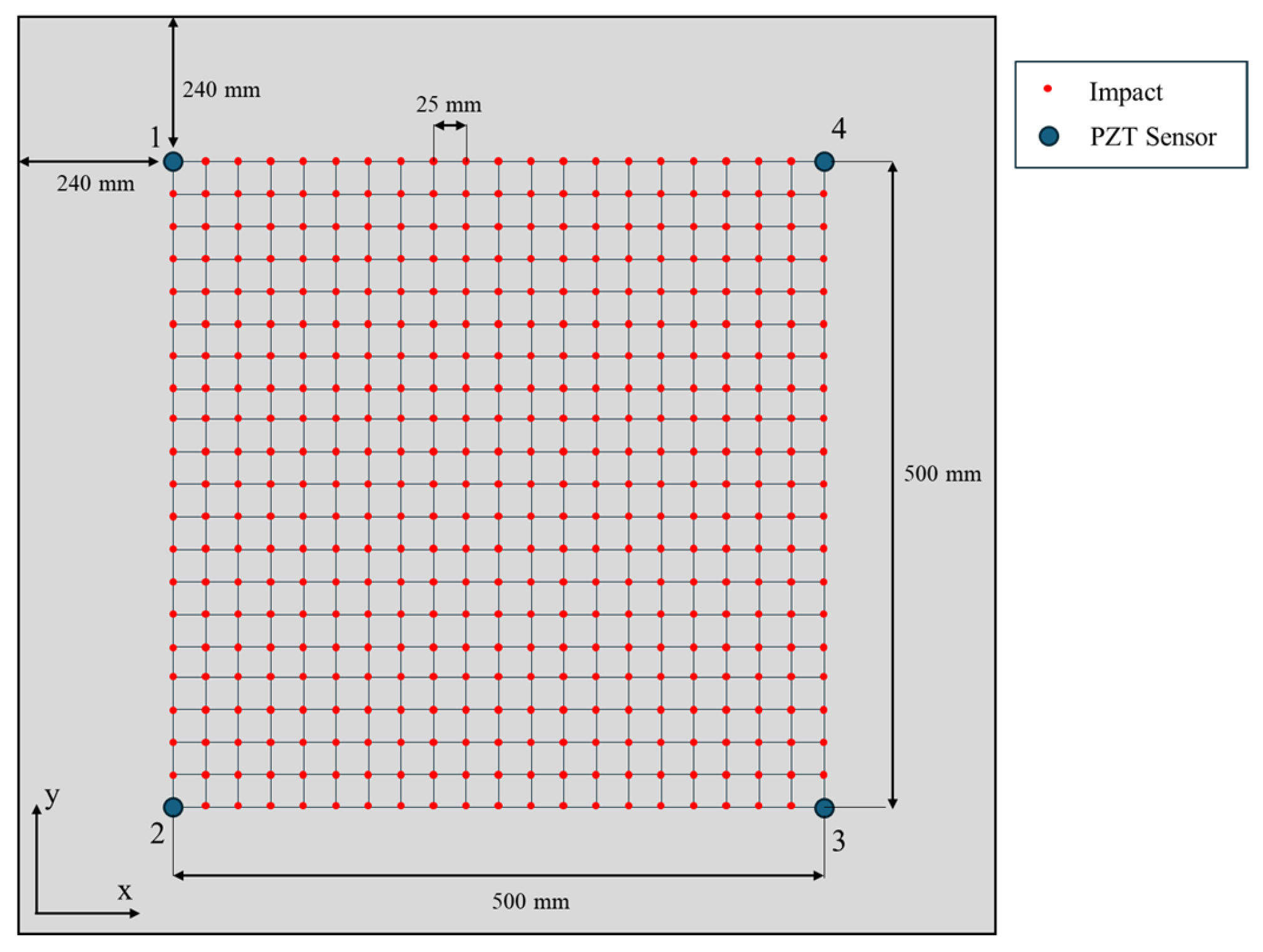
As shown in Figure 1b, for detecting the impacts, four PZT (Pb[Zr_xTi_1−x]O₃) piezoelectric ceramic sensors are secured to the plate surface using bicomponent epoxy glue. The sensor model is PIC255 by Physik Instrumente (Physik Instrumente, Karlsruhe, Germany) [22], characterized by a diameter of 10 mm. The PZT sensors are positioned at the corners of a square with a side length of 500 mm. The sensors are placed 240 mm from the edges of the plate. This placement helps to ensure a cleaner initial impact signal. The reverberations due to the edges are delayed since the impact wave travels 240 mm + 240 mm before being registered by the sensor.

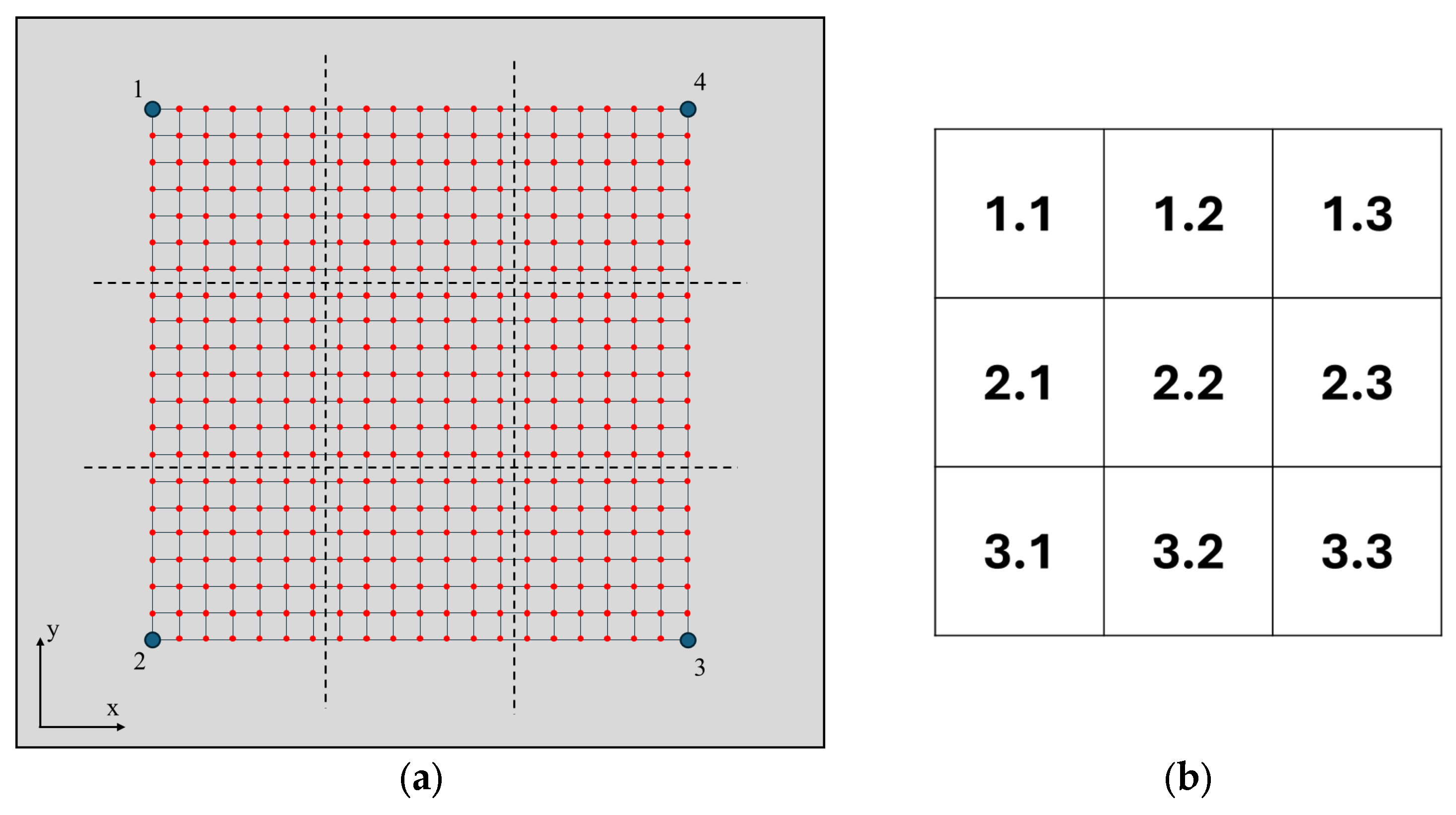
As depicted in Figure 2, a regular grid of 21 × 21 points defines the impact locations on the aluminum plate in the experimental tests, where the four positions (positions 1, 2, 3, and 4) at the vertex of the squared grid are occupied by the sensors. In total, 441 − 4 (sensor positions) = 437 impact points are realized on the component surface, at 25.0 mm from each other.

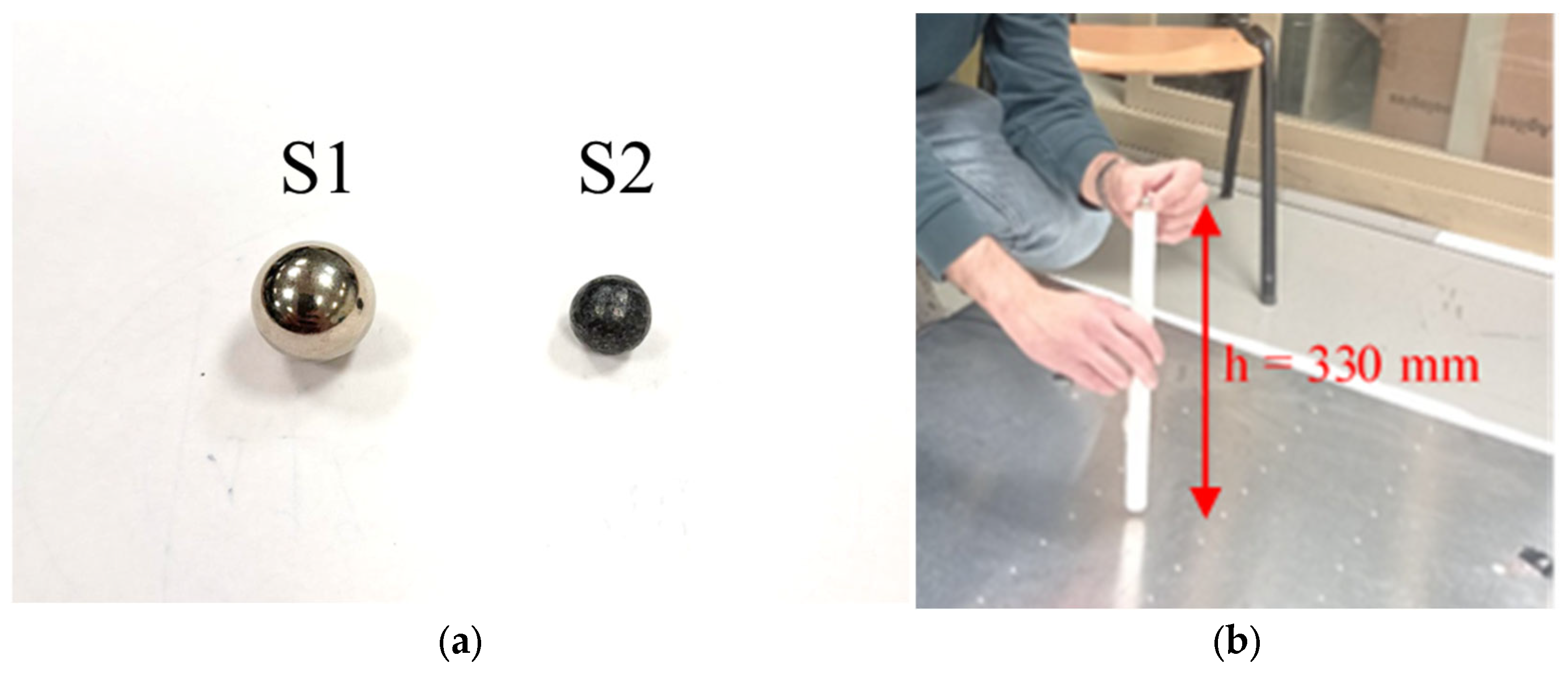
For generating the impacts, two spheres, namely S1 and S2, with different masses, are dropped on the plate surface. S1 is an 8.3 g stainless-steel sphere with a diameter of 12.6 mm, while S2 is a 3.6 g lead sphere with a diameter of 8.5 mm. As shown in Figure 3b, these are dropped from a fixed height of 330 mm using a tube for guiding the fall of the spheres at each impact point.

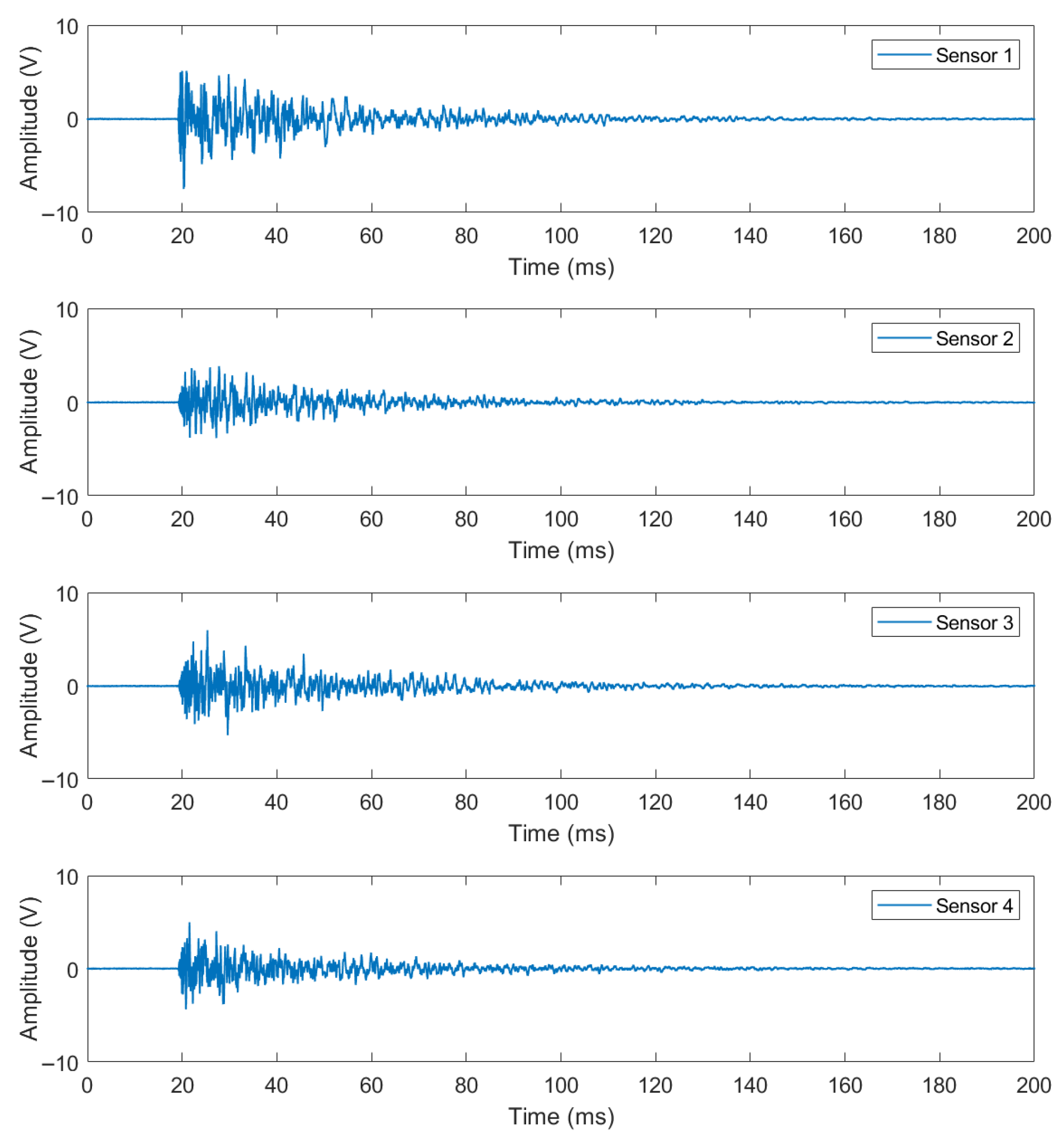
The data from the four PZT sensors are acquired using a Siglent (Siglent, Shenzhen China) SDS824X HD 4-channel oscilloscope, connected to a PC using an Ethernet cable to download the data. The sampling frequency of the signals is 5 MHz, and the resolution is 12 bit. The vertical scale of the oscilloscope is set to 10.0 V/div, allowing signals in range ± 40.0 V. To start the sampling, the acquisition channels of the oscilloscope are triggered with a threshold equal to 1.0 V. The total recording length is set to 200 ms including a pre-trigger of 20 ms. In this manner, in each signal, the whole impact phenomenon is acquired. It represents the impact event itself and the subsequent vibrations on the plate until it returns to a steady state. Even though the above-mentioned reverberations are not the object of this study, some considerations are added in the following paragraphs.

The test campaign includes 437 impacts repeated two times using sphere S1 and 437 impacts repeated two times using sphere S2. In total, 1748 impact signals are acquired from each PZT sensor.

2.2. Data Processing

In thin aluminum plates, only the zero-modes of Lamb waves, specifically the symmetric (S0) and antisymmetric (A0) mode, can be activated, and consequently, the acoustic emission frequency spectrum is predominantly concentrated below 100 kHz [21].

Previous research by the authors revealed that the signal’s arrival time, or Time of Flight (ToF), is primarily attributed to the A0 antisymmetric mode [10]. This is because the symmetric mode S0 exhibits negligible amplitudes within this frequency range. For this reason, the following analysis considers the Lamb waves in A0 mode at the specific frequency of 40 kHz.

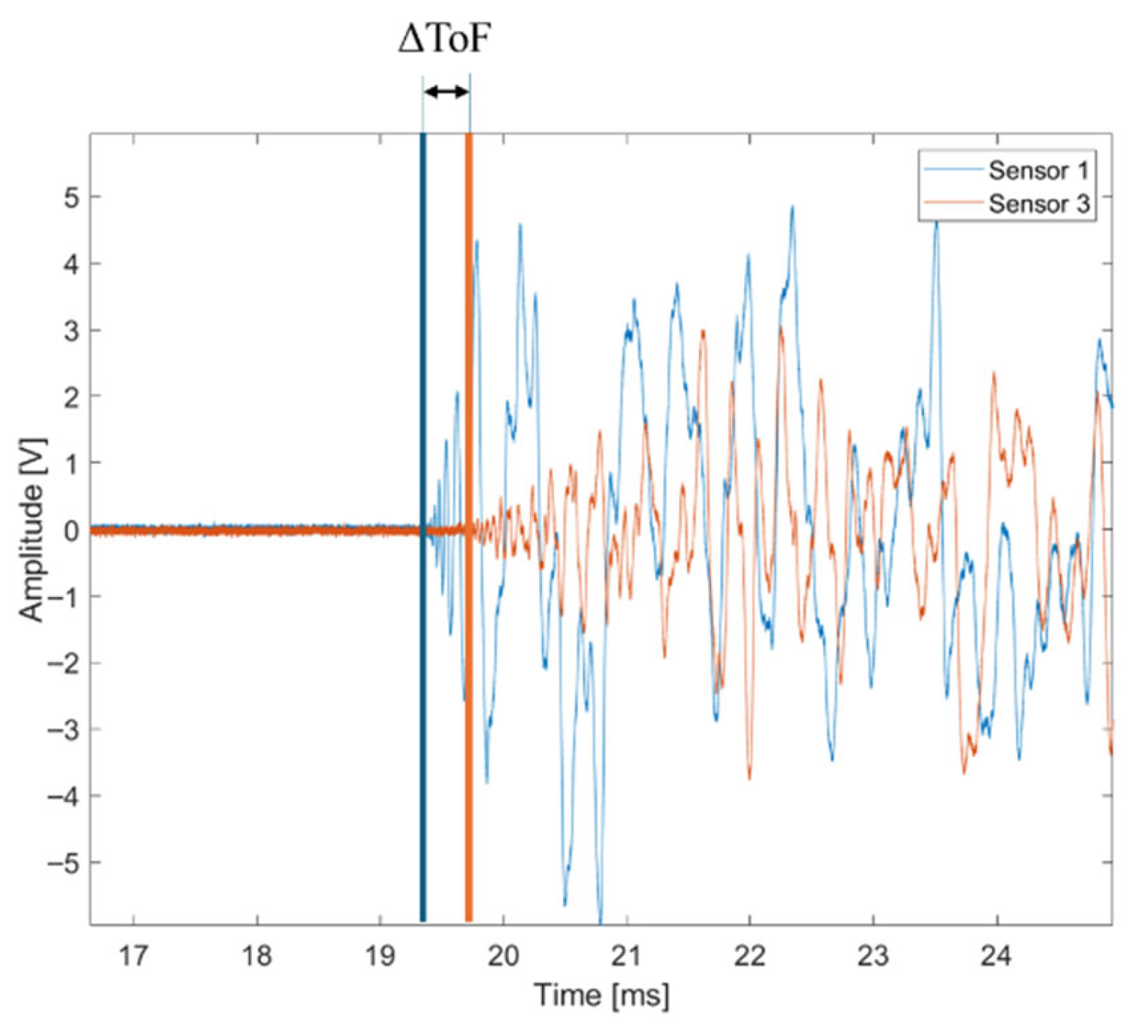
Since the exact time instant of impact cannot be determined, the ToF is assessed from the start of acquisition. To determine the impact location, the key parameter is the difference in ToFs (ΔToF) recorded by the PZT sensors. The ΔToFs are estimated using Cross Correlation (CC), Continuous Wavelet Transform (CWT), and Short-Time Fourier Transform (STFT). All of the data processing algorithms are implemented in MATLAB 2023b.

Figure 4 shows the impact signals measured by two sensors, demonstrating the ΔToF concept when sensor 1 (blue) and sensor 3 (orange) are considered. In this case, for instance, the two vertical lines indicate the temporal instance when the signals start changing from a steady state. It can also be noted that a pre-trigger condition is set on the oscilloscope, as already stated in Section 2.1. Measuring the difference in Time of Flight at the very beginning of the signal was found to be the most repeatable way; setting a threshold caused higher variability, probably since the starting slope at the beginning is not uniform depending on position.

2.2.1. Cross Correlation

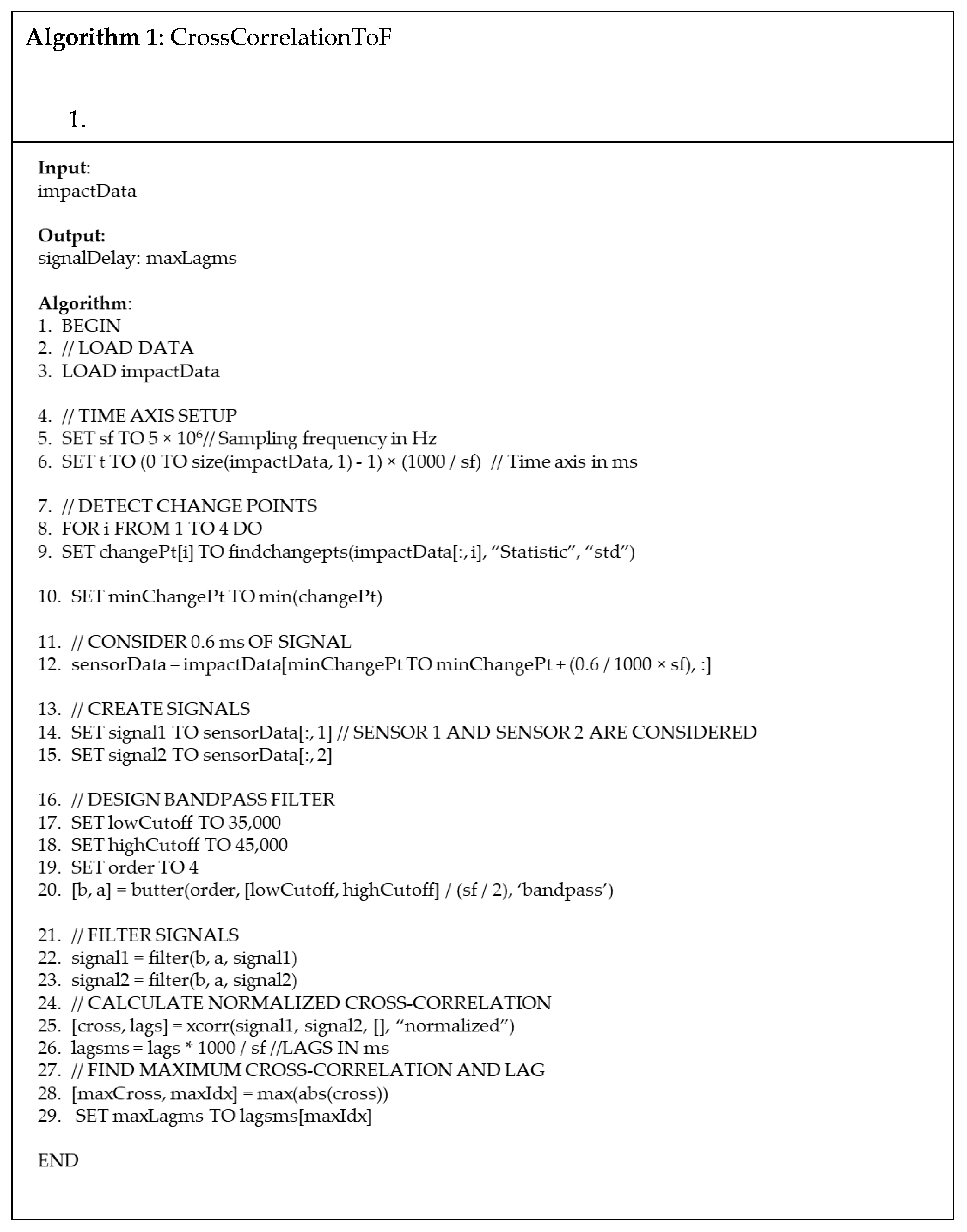
The oscilloscope signal is filtered using a bandpass Butterworth’s filter of order 4. The selected cutoff frequencies are 35 kHz and 45 kHz, enabling us to analyze only the 40 kHz signal component. This is the frequency at which a 1.5 mm thick aluminum plate has the maximum A0 mode amplitude [10]. Then, using the MATLAB built-in function findchangepts() [23], the data index where the signal changes most significantly is identified. The option used in this function is “std”, detecting changes in the standard deviation. The first instant of arrival of the wave at the four sensors is identified, and starting from this time point, considering the duration of the phenomenon, a time interval of 0.6 ms for all four acquired signals is selected for analysis. Considering an impact close to a sensor, 0.6 ms is the minimum time that it takes for the impact wave to travel from that point to the most distant sensor without introducing many reverberations in the first signal. The maximum distance found on the plate is 700 mm and the corresponding wave velocity is about 1135 m/s [10].

Successive waves are due to reflections and reverberations of the impact inside the plate. However, the selected signal length reduces unwanted vibrations. These signals are compared in pairs by calculating the CC coefficient [24]. The Cross Correlation coefficient peak corresponds to the associated delay between the two signals, which is the ΔToF. This procedure is repeated for all six sensor pairs.

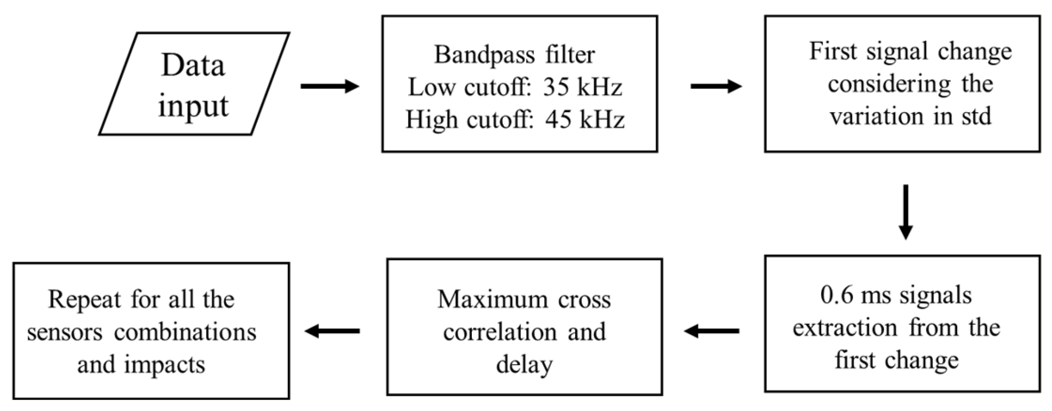
The flowchart of this procedure is represented in Figure 5.

2.2.2. Continuous Wavelet Transform

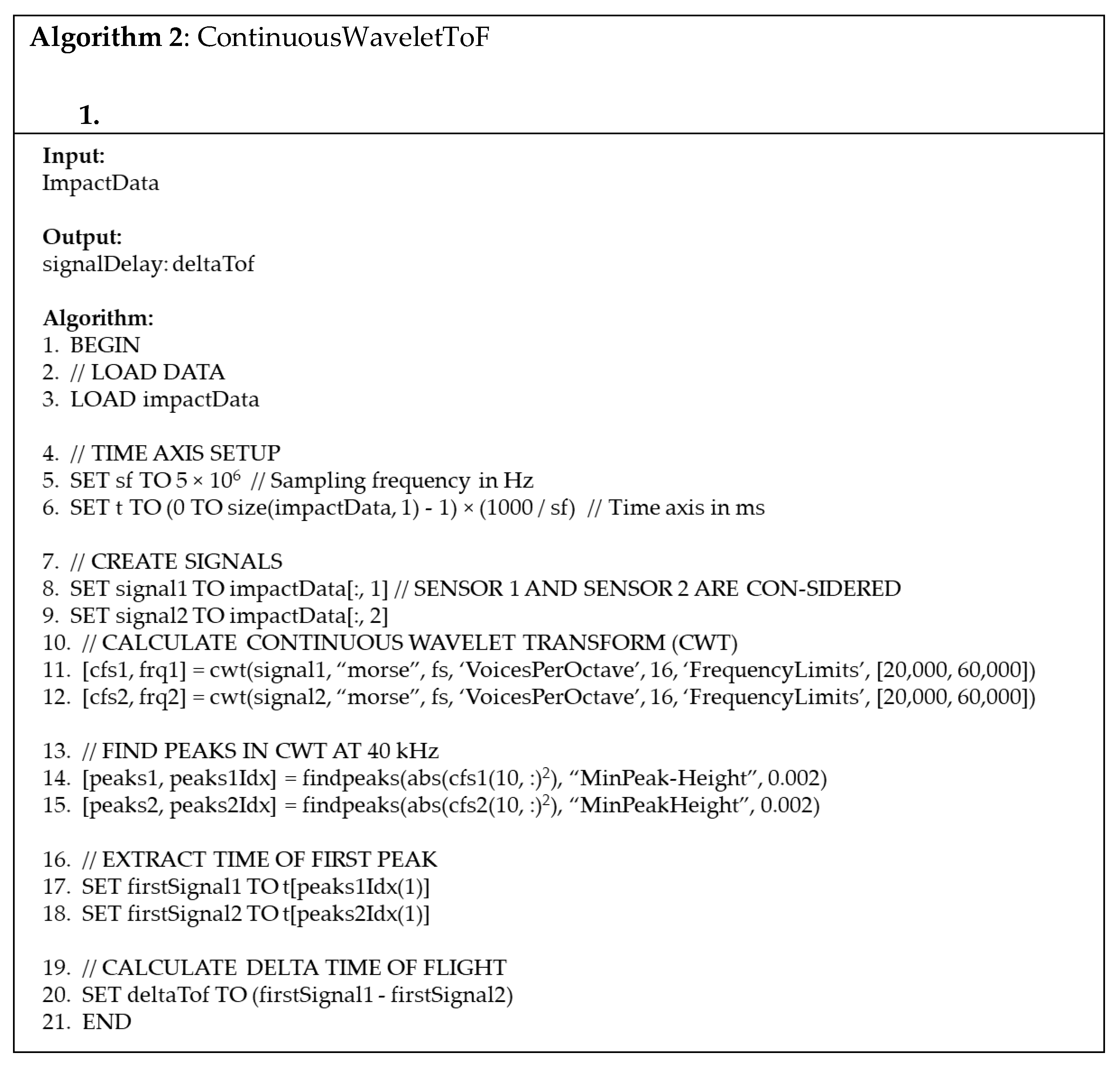
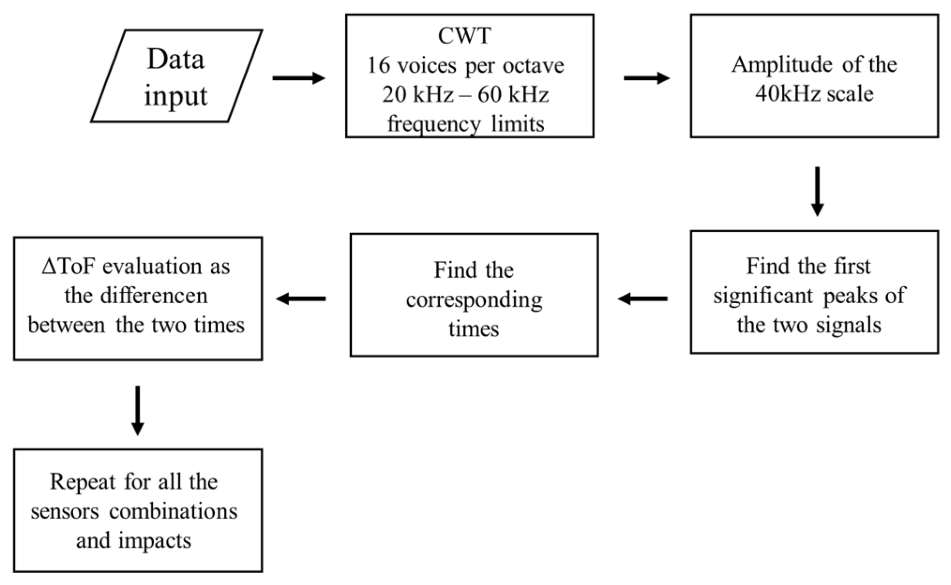
The impact signal for each sensor is analyzed using CWT to extract both time and frequency information. CWT uses a mother wavelet that is scaled and shifted to provide different window sizes for different frequencies. In this case, the CWT of the signal is computed in frequencies starting from 20 kHz to 60 kHz using Morse wavelets with a symmetry parameter equal to 3 and a time-bandwidth product equal to 60. This type of wavelet is considered useful in localizing discontinuities in signals [25]. To better represent the signal, the wavelet is computed using 16 voices per octave. The amplitude of the scale closer to the target frequency is considered, and its squared modulus is calculated. The impact instant is the time that corresponds to the first significant peak in the scalogram. The ΔToFs are the differences between the time instants identified for each sensor. All of these steps are summarized in Figure 6.

2.2.3. Short-Time Fourier Transform

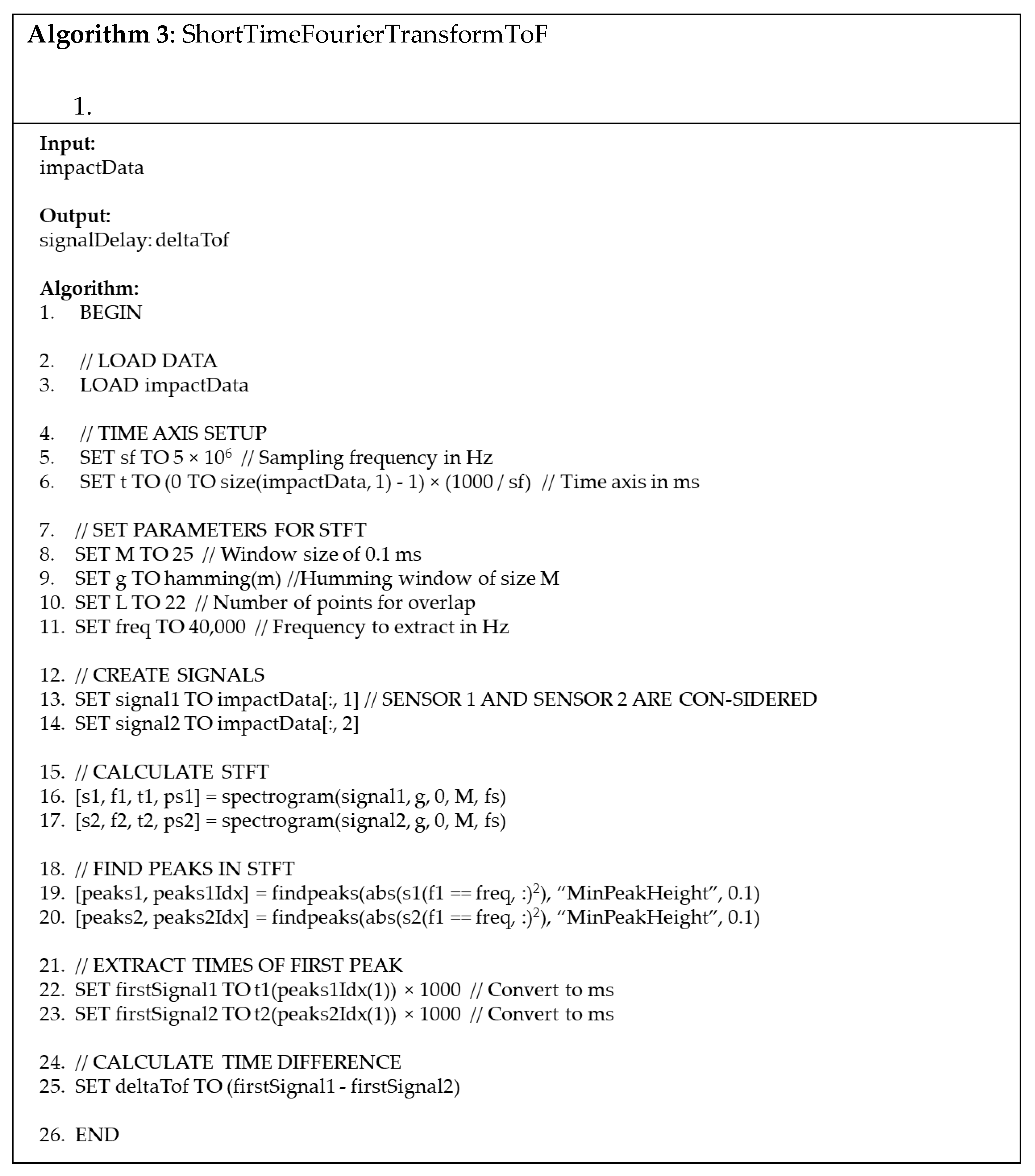
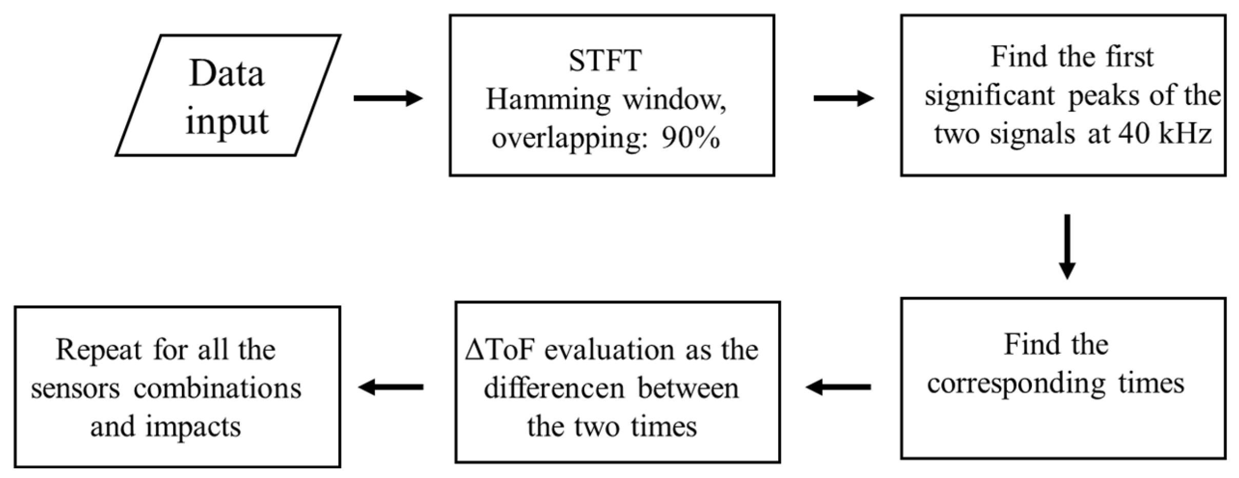
Calculating STFT, the signal is analyzed both in time and frequency domains. In this case, the window length is 0.1 ms and the corresponding frequency resolution is equal to 10 kHz. In STFT, the window length is fixed for all frequencies. Selection of the window length must balance the necessity of frequency and time resolution. To reduce leakage, hamming windows are used with 90% overlapping. The ToF is calculated considering the amplitude of the signal corresponding to 40 kHz. Then, the local peaks of the energy at this frequency are identified using the built-in Matlab function findpeaks() [26]. This function identifies local maxima in a signal vector depending on the option ‘MinPeakHeight’, which is employed for refining the findings of the peaks. In this case, this option is activated to reduce the effect of initial noise on the measured signal. The first notable peak in the signal is recognized as the impact instant. Therefore, its time of occurrence indicates the ToF for each sensor, and the ΔToFs are determined considering all sensor pairs for each impact point.

The variability in each ΔToF estimation is calculated with reference to each sensor pair considering four repeated impacts and assuming a uniform distribution [27].

The calculated ΔToFs considering all points and all repetitions represent the predictors for localizing impacts using Machine Learning approaches.

Figure 7 illustrates ΔToF estimation using the STFT methodology.

2.3. Machine Learning Models

This work focuses on using classification algorithms applied to the impact ΔToFs for identifying the regions of the plate where impacts occurred.

Since there are many possible classification models for this task and it is not possible to identify the best one a priori, multiple models are trained and compared in terms of classification accuracy.

2.3.1. Definition of Classification Zones

The definition of the plate zones is based on geometrical considerations to avoid biases in classification using ML algorithms. In this case, the impact point distribution is uniform on the surface; so, in each sub-area, there is the same number of points. This aspect is important for generating a training dataset that does not present class imbalances.

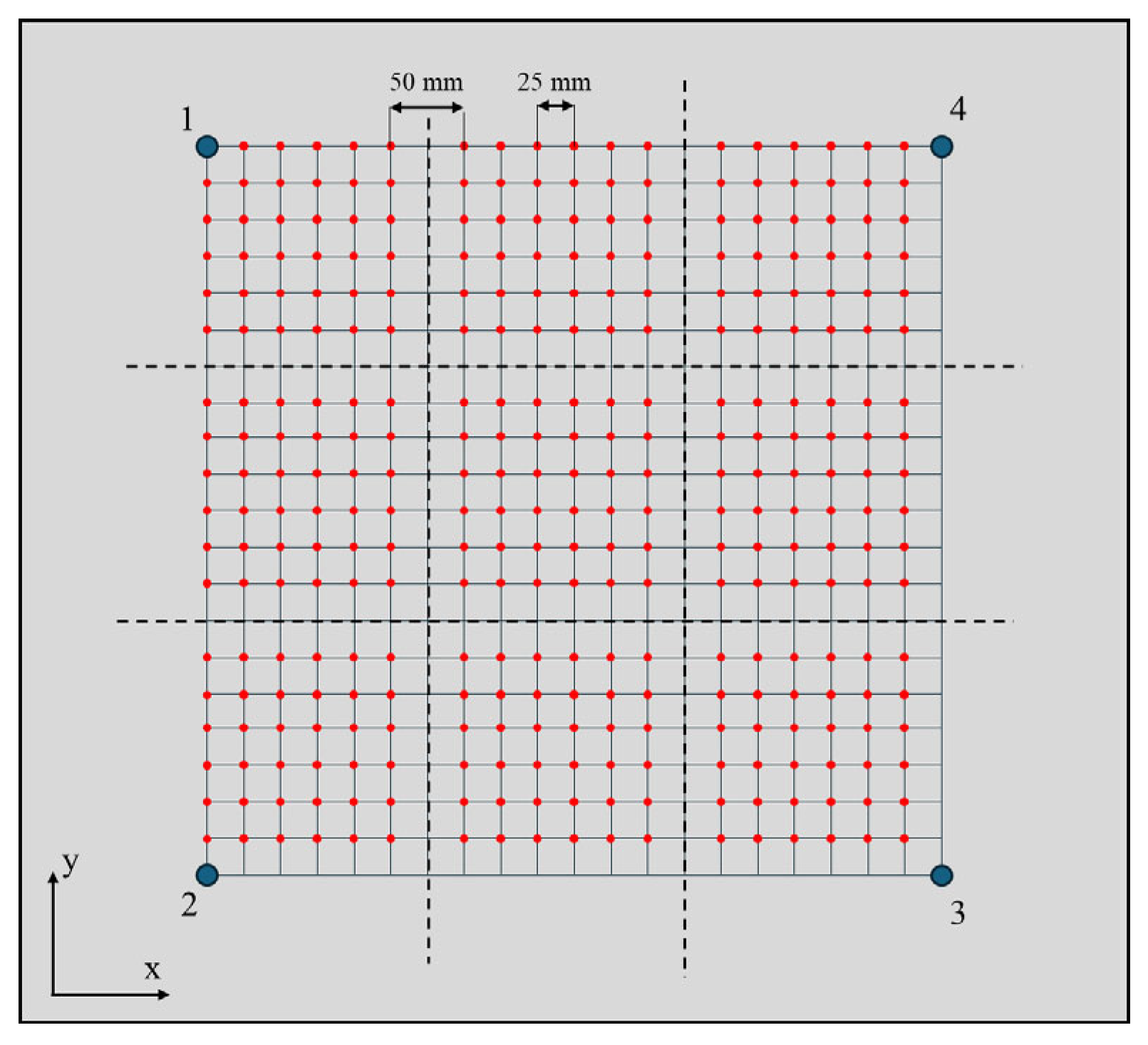
The aluminum plate surface is subdivided considering a matrix of 3 × 3 elements, resulting in 9 impact zones. Figure 8 shows the subdivision of components.

The impact points are in a square measuring 150 × 150 mm. Using this subdivision, the number of impact points is balanced for each zone and equal to 49, or 48 for areas positioned at the edges, where a position is occupied by the PZT sensor. A representation of the zone nomenclature is reported in Figure 8b.

2.3.2. Effect of Impact Points Configuration

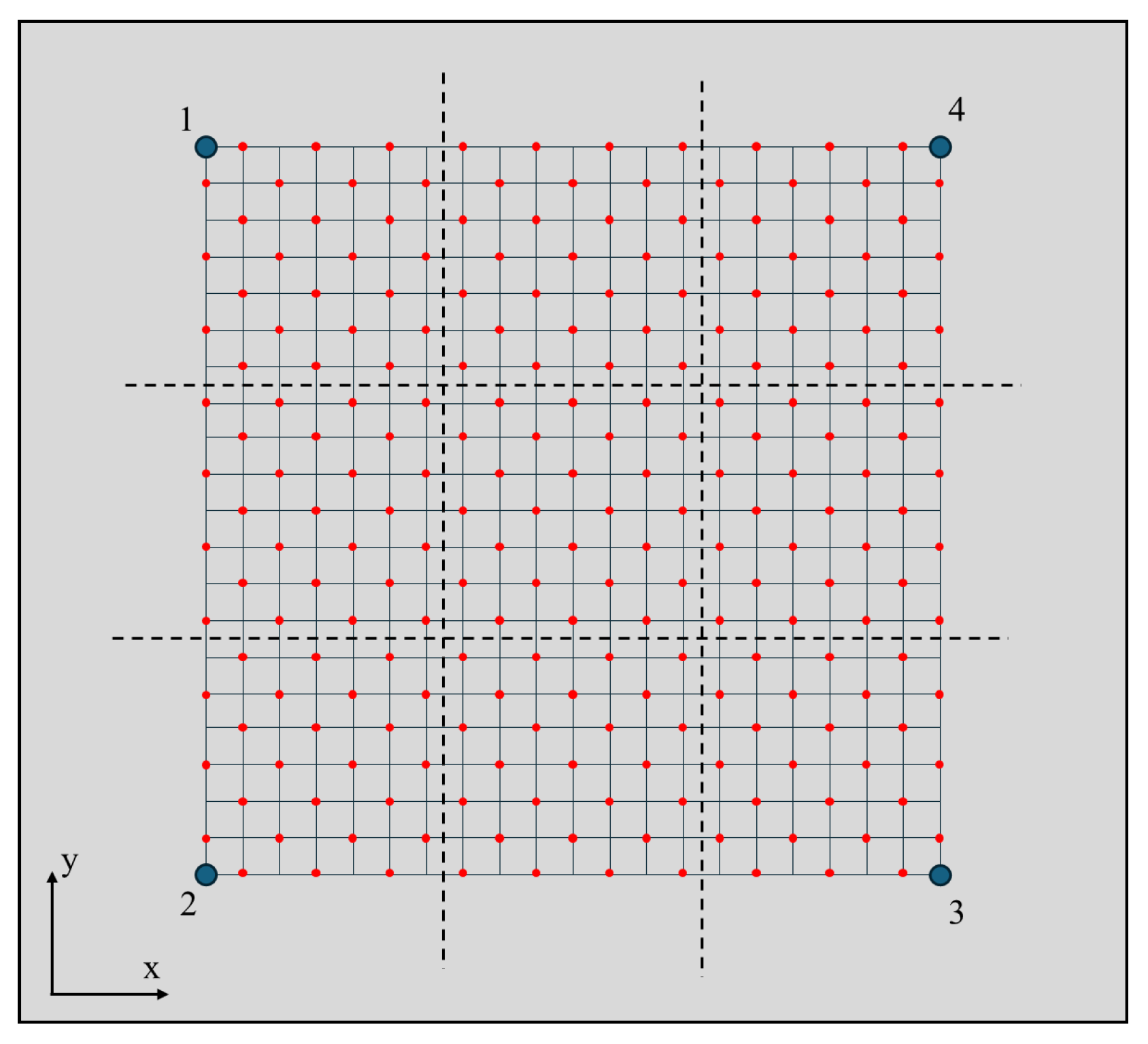
The points near the borders are the most critical. To evaluate their effect, a different point configuration is considered that excludes them. Each zone is redefined as shown in Figure 9.

In this configuration, points that are located less than 25 mm from the border are not considered. Compared to the previous case, the dataset is 70% of the original one.

2.3.3. Effect of Number of Points

The effect of the amount of data used for training on classification performance is assessed by considering half impact points. Figure 10 represents the distribution of the impact points used in this analysis.

With the impact points distributed as shown in Figure 10, along with data reduction, the minimum distance between two points is equal to ~35.4 mm, i.e., the diagonal of the square with dimensions of 25.0 mm.

2.3.4. Effect of Signal Sampling Frequency

Signal sampling frequency is important for several aspects of this analysis. First, it defines the maximum frequency that could be analyzed, according to the Nyquist theorem. Secondly, it influences the number of data points recorded and the further computational cost for ΔToF estimation. To evaluate the effect of the sampling frequency, the original 5.00 MHz signal is resampled to 1.00 MHz and 500 kHz. To perform signal resampling, the MATLAB resample() [28] function is used, allowing the input signal to be resampled with a pre-defined ratio between positive integers. This means that not only the input signal but also the constants ‘p’ and ‘q’ are provided; so, the function resamples the input sequence at p/q times the original sample rate.

2.3.5. Reproducibility of Results

To verify the robustness of the classification methods developed in this work with the aim of assessing the reproducibility of the results obtained, the impact signals acquired using a different experimental setup are analyzed. In particular, the same aluminum plate along with the PZT sensors is used for recording 167 impact signals. In this case, the data are sampled at 3.96 MHz using a different instrument [10] and the impacts are generated with bodies of different masses. To maintain the vibrational behavior of the plate, it is put on the same foam material.

The provided impact signals are then analyzed using the three developed methods and the corresponding ΔToFs are classified using the trained models.

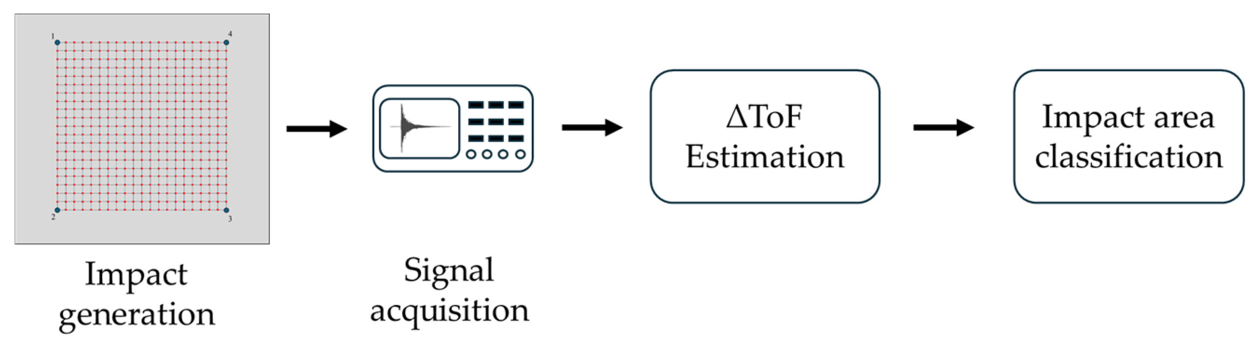
Figure 11 shows a reference scheme of the general flowchart described in this paper. Regarding the ΔToF estimation methods, these are better described in Appendix A, where the pseudocodes are provided for each technique.

3. Results

Using the experimental setup outlined in the previous section, an example of the temporal signals acquired during a single impact is presented in Figure 12.

In this section, the results of the ΔToF estimation methods and the training of classification models are presented. As stated in Section 2, the influencing factors analyzed are as follows:

• ΔToF estimation method.
• Classification model.
• Layout of impact points.
• Sampling frequency of signals.

3.1. Differences Among ΔToF Estimation Methods

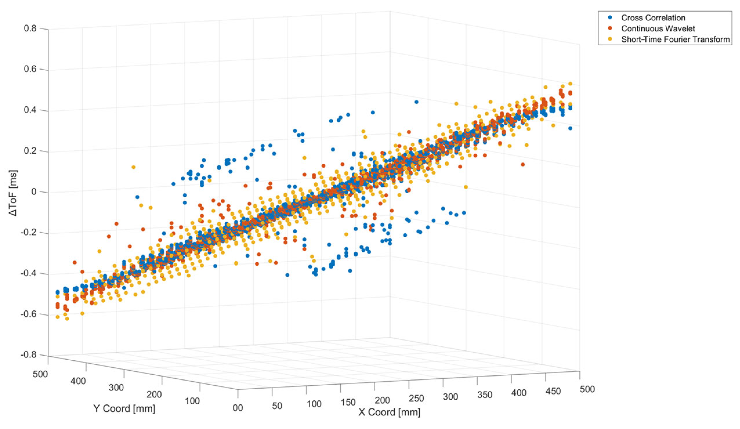
Figure 13 shows the estimations of the ΔToFs of a pair of sensors using the three different methods and considering both spheres for generating the impacts. The impact point coordinates as defined on the aluminum plate are represented on the X and Y axes, while the ΔToFs are reported on the Z axis.

In this case, the ΔToFs of sensor 1 and sensor 3 in a pair are reported, placed on the diagonal of the regular grid. Sensor 1 is the reference and has coordinates (0, 500) while sensor 3 is placed at (500, 0). Since the plate material is homogeneous with no discontinuities, the wave velocity inside it is constant. Consequently, the ΔToFs of the sensors placed on the diagonal are distributed on a plane, as can be seen in Figure 10.

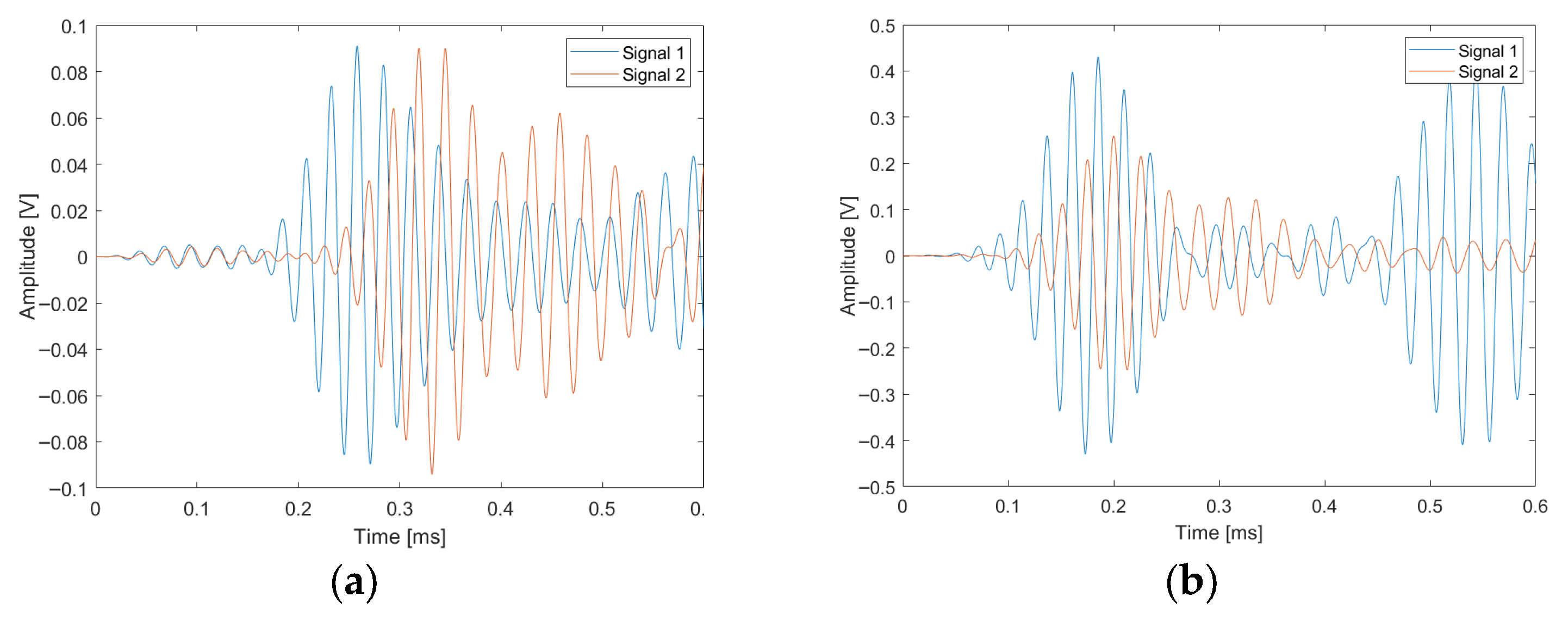
CC is the method that presents more points that deviate more from the ideal behavior, clearly visible in Figure 10. This result is due to the method used for extracting the initial part of the signal. In some cases, in fact, the selected signal length also includes reverberations that affect the analysis. Figure 14 reports examples of different signals analyzed using the CC method. Figure 14a shows a signal where only the initial part of the impact is extracted, while Figure 14b represents a case where there are also some reverberations. It has to be noted that the represented signals are from two different impacts.

Considering the ΔToFs estimated using STFT, the values are more diffused along the ideal fitting plane of the points shown in Figure 13. This is due to the temporal resolution linked to the selected window length.

For CWT, the points are closer and less diffused near the ideal plane due to the better temporal resolution of this method.

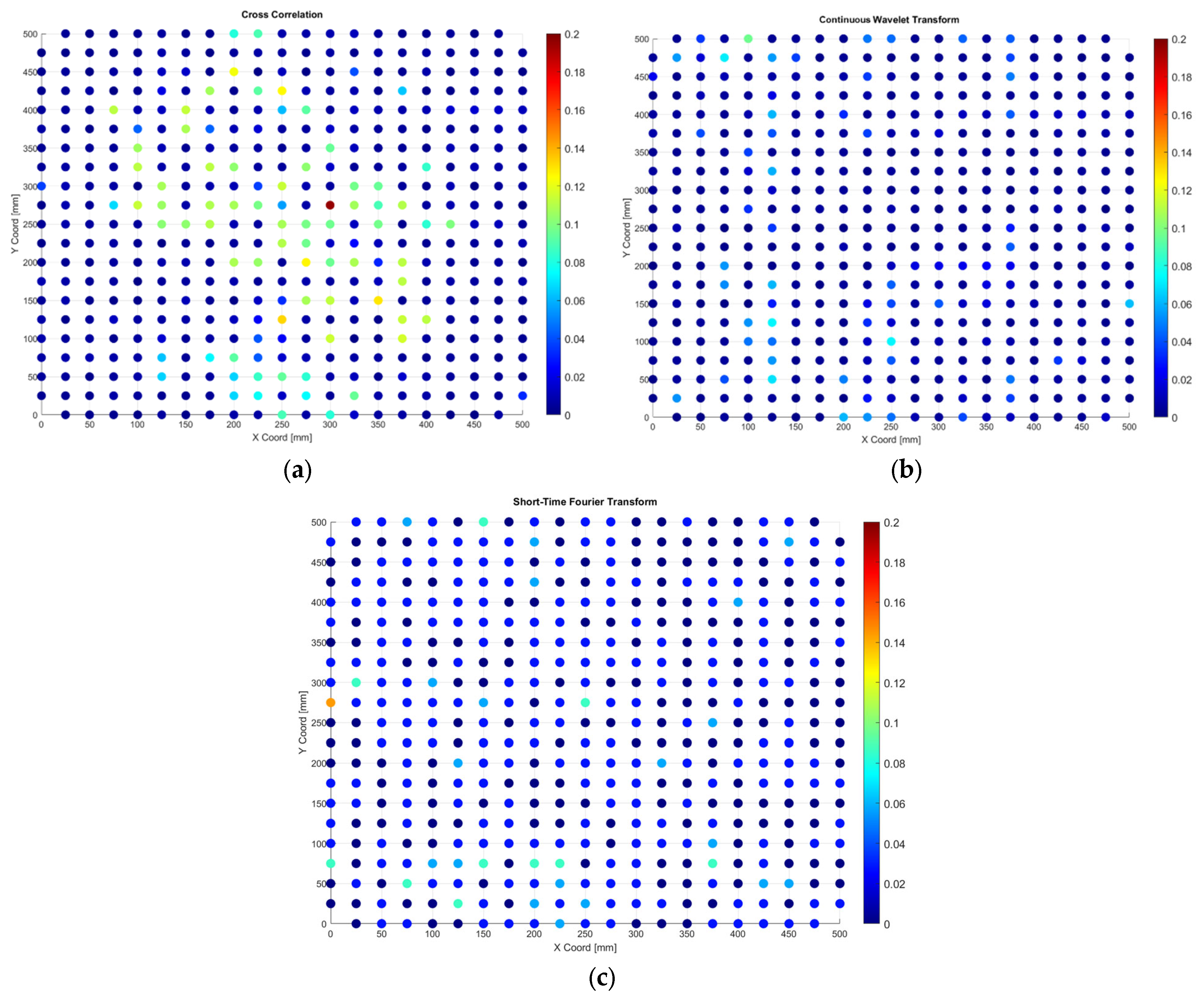
The variabilities of the ΔToFs are evaluated across four repeated impacts in all locations. In Figure 13, as an example, the ΔToF variability of sensor pair 1–3 is reported for each estimation method.

For CC in Figure 15a, ΔToF variability values are in the range from 0.0004 ms to 0.20 ms. The greater variability is acknowledged in the direction of the line connecting the two sensors, along the diagonal of the grid. The same behavior occurs considering the other pairs of sensors. This appears to be a consequence of the signal extraction method used for selecting which part to analyze, as described in Section 2.

The ΔToFs estimated using the CWT method have a minimum variability of 0.0002 ms and a maximum value of 0.0974 ms. The impacts with greater variability appear to be randomly distributed on the grid.

Finally, the minimum variability of STFT is equal to zero while the maximum value is 0.14 ms. Also, in this case, point variability distribution does not present a regular pattern.

The mean ΔToF variability of the different estimation methods is summarized in

Table 1. Mean variability of different ΔToF estimation methods.

ΔToF Estimation Method	Mean Variability [ms]
CC	0.012
CWT	0.008
STFT	0.019

.

As reported in Table 1, CWT presents less variability compared to the other two approaches.

A repeatability test is performed, repeating 20 impacts on one location and considering the signals from sensor 1 and sensor 3. The ΔToFs are calculated using the three estimation methods and the repeatability is calculated considering the standard deviation. The repeatability of the ΔToFs estimated using CC is equal to 0.009 ms, while with CWT it is 0.002 ms and using STFT it is 0.030 ms. These results are satisfactory and prove that the handheld tube with careful positioning ensures the repeatability of the impacts within a maximum variability of 4–6%.

3.2. Classification Models

As described in the previous section, the dataset is composed of 1748 impact signals, of which 80% are used for training while 20% are for model testing. To avoid overfitting, a k-fold cross-validation scheme is employed, partitioning the training dataset into five subfolders.

The features used as input of the classification models are the six ΔToFs from all sensor pairs, while the output is the impact zone.

A classification model is trained for each ΔToF estimation method, and different ML models are trained to find the best one. Testing accuracy is used as the first comparison metric of the different classifiers.

Table 2. Performance of trained classification models.

ΔToF Data	Model	Validation Accuracy [%]	Testing Accuracy [%]
CC	Ensemble Subspace KNN	94.3	93.7
CWT	Ensemble Boosted Trees	97.2	98.0
STFT	Weighted KNN	85.6	85.7

summarizes the performance of the trained classification models.

The performance of the models varies depending on the ΔToF estimation method. For CC data, the best performing model is an Ensemble Subspace KNN, which utilizes K-Nearest Neighbors (KNNs) enhanced by subspace and ensemble learning. It trains 30 KNN classifiers on different subsets of data with fewer features to improve performance. Considering CWT data, an Ensemble Boosted Trees model is used. This is composed of 30 decision trees trained using the AdaBoost algorithm. Finally, for STFT ΔToFs, the selected model is a Weighted KNN trained with 10 nearest neighbors. The weights for each of them are the squared inverse of the Euclidean distance.

Comparing the different ΔToF estimation methods, the model trained on the CWT data provides the best results with a classification accuracy of 98%. This is a consequence of the reduced variability of the ΔToFs, as shown in the previous section. For all trained models, the 5-fold cross-validation scheme avoids overfitting since the validation and testing accuracies are similar.

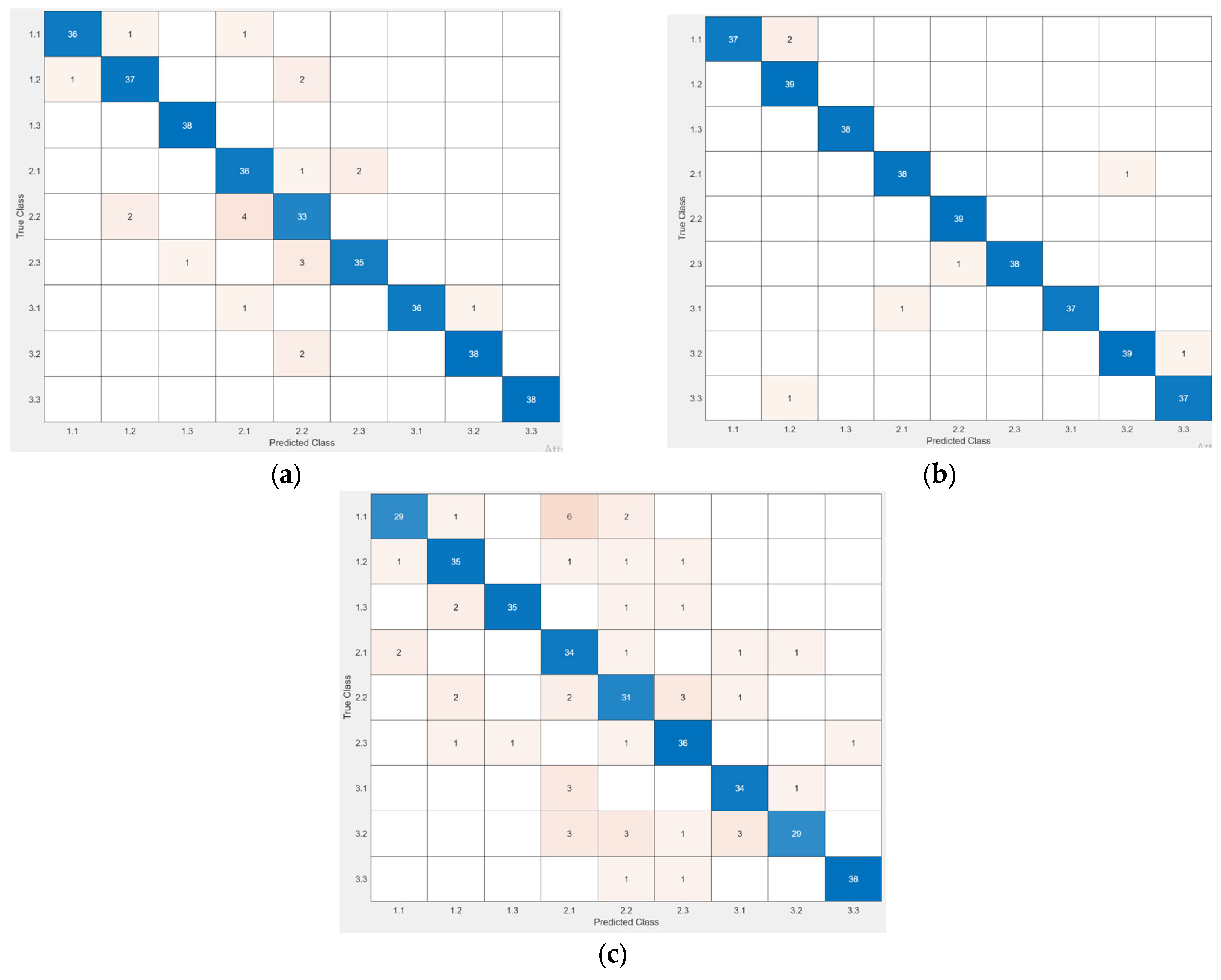
Figure 16 represents the confusion matrixes of the trained models in the testing phase, enabling us to better understand the classification capabilities of each trained model.

From the confusion matrixes reported in Figure 16, for CC- and CWT-trained models, wrongly classified impacts are mostly localized in zones adjacent to the real one. The zone that is affected the most by this effect is 2.2, since it borders all the others. Considering the model trained using ΔToFs estimated with STFT (Figure 16c), there are several classification errors and many of them are not localized in nearby zones due to STFT frequency and time resolution.

3.2.1. Effect of Impact Point Layout

The effect of impact point layout is evaluated by removing the points on the borders of each zone. With this arrangement, errors due to the misclassification of impacts in zones close to each other are reduced.

Table 3. A summary of the accuracy of the classification models trained using all impact points and removing the points on borders.

	All Points		No Points on Borders
ΔToF Data	Validation Accuracy [%]	Testing Accuracy [%]	Validation Accuracy [%]	Testing Accuracy [%]
CC	94.3	93.7	97.0	95.7
CWT	97.2	98.0	97.6	98.8
STFT	85.6	85.7	90.8	89.5

summarizes the accuracy of the trained models using all impact points and the dataset without data on the borders.

As reported in Table 3, by removing the points on the borders, an increment in validation and testing accuracy is observed for all classification models. This is due to the reduction in misclassification errors in contiguous zones.

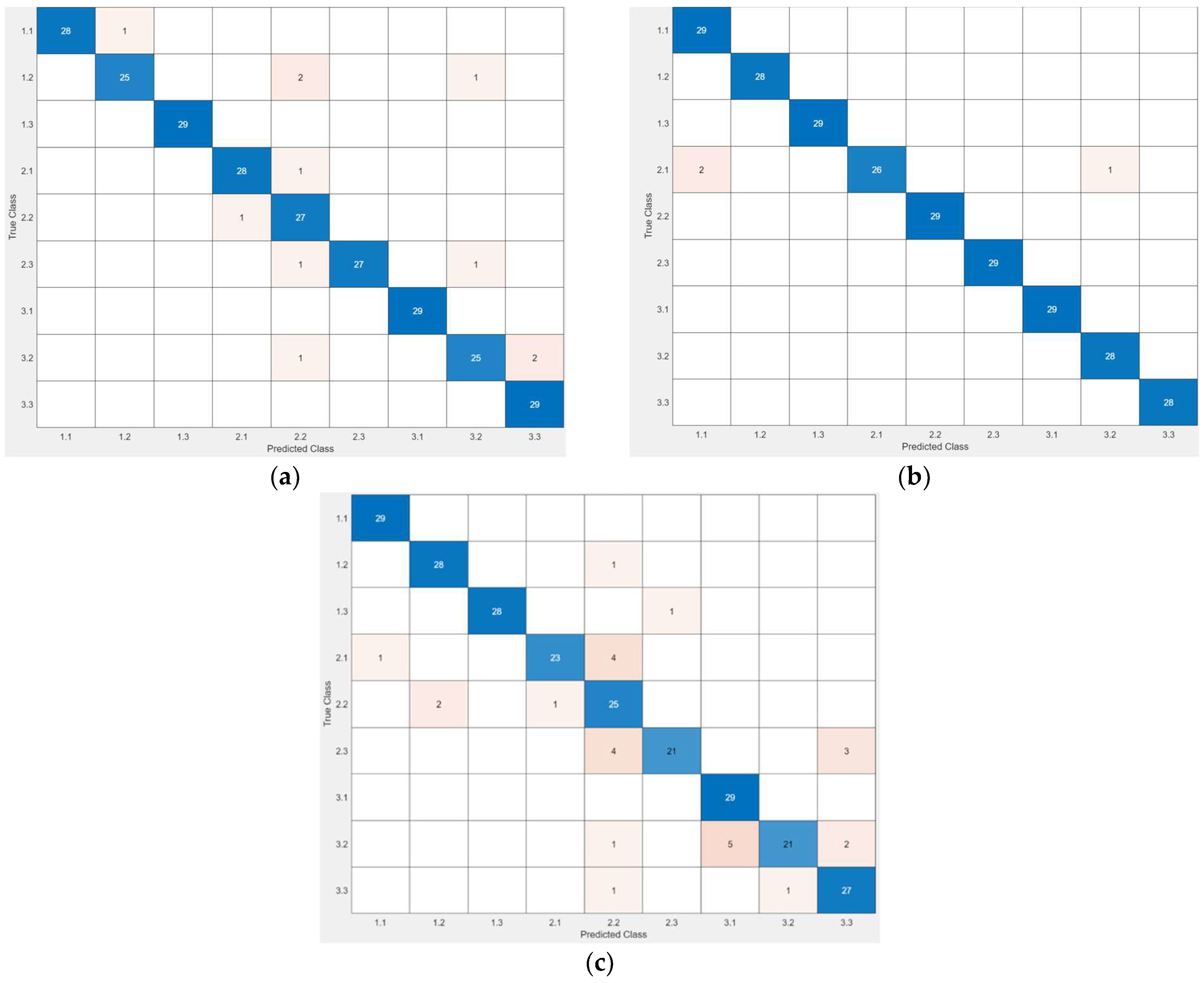
In Figure 17, the confusion matrixes of the models are reported.

As shown in Figure 17, there is a reduction in errors in contiguous zones for all models. However, as shown in Figure 17a, zone 2.2 still has different impacts classified in zones next to it. As shown in Figure 17c, eliminating the points on the border also improves the performance of the STFT model.

3.2.2. Effect of Number of Impact Points

The effect of the number of points used for training is evaluated by considering half impacts and a minimum distance between points of 35.35 mm.

Table 4. A summary of the accuracy of the classification models trained using all impact points and only half of the dataset.

	ALL POINTS		HALF POINTS
ΔToF Data	Validation Accuracy [%]	Testing Accuracy [%]	Validation Accuracy [%]	Testing Accuracy [%]
CC	94.3	93.7	93.0	94.3
CWT	97.2	98.0	95.9	96.6
STFT	85.6	85.7	83.9	88.1

reports the comparison between the accuracies of the classification models trained using all impact points and using only half of the dataset.

As shown in Table 4, no significative effects are observed due to the reduction in impact points.

3.2.3. Effect of Sampling Frequency

In

Table 5. A summary of the accuracy of the classification models trained using a dataset with different sampling frequencies.

	5 MHz		1 MHz		0.5 MHz
ΔToF Data	Validation Accuracy [%]	Testing Accuracy [%]	Validation Accuracy [%]	Testing Accuracy [%]	Validation Accuracy [%]	Testing Accuracy [%]
CC	94.3	93.7	94.1	93.4	94.0	93.1
CWT	97.2	98.0	96.9	95.7	97.7	97.7
STFT	85.6	85.7	86.2	85.7	86.8	82.5

, a summary of the accuracies of the models trained using subsampled signals is reported.

For all of the trained classification models, no significant variations are observed in the accuracy of the classification models. This is aspect is of great interest in terms of reducing the computational cost of the analysis, which required further analysis compared to previous works [10]. A previous study focused on a regression analysis for impact localization, which exploited the maximum sampling frequency of 5.0 MHz provided by the oscilloscope. Identification of the impacted area with lower acquisition and computational costs was confirmed. This represents a promising result for the optimization of the overall procedure, since the accuracy of classification is a global indicator, accounting for sampling frequency effects as well as the other effects analyzed.

3.2.4. Reproducibility Assessment

To verify the reproducibility of the analysis and further test the classification models, the above trained classification models are used with a different ΔToF dataset, obtained by means of tests carried out in a different laboratory under similar but not identical conditions; the models were trained with three datasets: one considering the total number of points, one excluding the points near the borders, and one using half of the points.

The results in terms of the accuracy of this analysis are summarized in

Table 6. Classification accuracies using trained models on different datasets.

Model	TRAINING DATASET
	All Points	No Borders	Half Points
CC	94.6	91.0	79.6
CWT	94.6	95.2	86.2
STFT	79.6	77.2	80.2

.

The models trained with the ΔToFs estimated with CWT proved to be the most accurate with respect to changes in the experimental setup. They showed satisfactory reproducibility even when challenged by a reduction in the number of training points. In the case of CC, a high sensitivity to the reduction in the number of points was highlighted. On the other hand, the STFT model showed less reproducibility when different experimental setup datasets were used as input. This outcome is probably due to the worse temporal resolution of the method.

Our results show that the models trained using CWT as the ΔToF estimator are more robust to reductions in training data and can classify impact signals acquired with a different setup while providing satisfactory accuracy. This promising outcome regarding the reproducibility of data processing and analysis is a relevant result for in-field implementation.

Therefore, as a final consideration, the aspects with the greatest impact on classification accuracy are the algorithm used to estimate the ToFs, the number of points used to train the ML models, the classification model chosen, the geometry of impact point distribution, and the balance of points across the classification areas; instead, a negligible effect was observed for acquisition frequency.

4. Conclusions

In this paper, the effects of different parameters were studied for classifying the localization of an impact on an aerospace component. The analysis of variability in different aspects of the methodology provides suggestions for improving the reproducibility of results. The main aspects that influence variability and bias errors in the results have been studied. These are related to the experimental procedure, such as the layout of the impact grid and its density, the shape of the impact areas to be classified, and the frequency of acquisition of data, and to the data processing technique, such as algorithms for estimating the differences in Times of Flight (ΔToFs) as well as ML classifiers and their parameters. Tests were carried out on an aluminum plate with four PZT sensors to acquire impact signals. Among CC, CWT, and STFT, it was found that CWT estimations of ΔToFs have the lowest mean variability, which is equal to 0.008 ms, and can be used as training features for different classification models. The optimized classification method shows a testing classification accuracy of 98%. Finally, these trained and improved models have been applied to datasets obtained in a different laboratory with the aim of studying the reproducibility of the results as well as the potential for an in-field transfer of the developed techniques. Our results show that the trained models exhibited an accuracy in the order of 95%, even though many testing conditions were changed such as the data acquisition system and the algorithm used to estimate ΔToFs, the data acquisition frequency, the operators, the impact spheres, and the laboratory environmental conditions. These results demonstrate the potential of the procedure not only for use with homogeneous materials but also for cases where more complex materials are such as in aerospace applications. Having quantitively assessed a possible benchmark for a data-driven ML approach for SHM application, the next step is to integrate it with advanced analytical models. This step is necessary for analyzing more complex components, such as composite plates made of carbon fiber or wing-shaped parts and reinforced components with screw holes. Indeed, the application of this procedure to more complex materials will be a further step in this project’s work.