Characterization of the Extraction System of Supersonic Gas Curtain-Based Ionization Profile Monitor for FLASH Proton Therapy

Abstract

FLASH radiotherapy requires real-time, non-invasive beam monitoring systems capable of operating under ultra-high dose rate (UHDR) conditions without perturbing the therapeutic beam. In this work, we characterized the extraction system of Supersonic Gas Curtain-based Ionization Profile Monitor (SGC-IPM) for its capabilities as a transverse beam profile and position monitor for FLASH protons. The monitor utilizes a tilted gas curtain intersected by the incident beam, leading to the generation of ions that are extracted through a tailored electrostatic field, and detected using a two stage microchannel plate (MCP) coupled to a phosphor screen and CMOS camera. CST Studio Suite was employed to conduct electrostatic and particle tracking simulations evaluating the ability of the extraction system to measure both beam profile and position. The ion interface, at the interaction region of proton beam and gas curtain, was modeled with realistic proton beam parameters and uniform gas curtain density distributions. The ion trajectory was tracked to evaluate the performance across multiple beam sizes. The simulations suggest that the extraction system can reconstruct transverse beam profiles for different proton beam sizes. Simulations also supported the system’s capability as a beam position monitor within the boundary defined by the beam size, the dimensions of the extraction system, and the height of the gas curtain. Some simulation results were benchmarked against experimental data of 28 MeV proton beam with 70 nA average beam current. This study will further help to optimize the design of the extraction system to facilitate the integration of SGC-IPM in medical accelerators.

1. Introduction

FLASH proton therapy promises radiotherapy with effective sparing of normal tissues while covering the tumor as efficient as in conventional proton therapy [1,2,3,4,5]. This treatment modality requires UHDR in the order of 40 Gy/s, which poses challenges in both accelerator technology and beam diagnostics. Laser-driven proton acceleration is one such accelerator technology capable of delivering FLASH protons, which can scale down the enormous infrastructure of existing medical proton accelerators [6,7,8]. Under FLASH conditions, real-time beam monitoring becomes essential for achieving precise dosimetry, due to the treatment delivery time of a few fraction of seconds [9,10]. Beam diagnostic tools, such as radiochromic films, Faraday cups, Ionization Chambers (ICs), and Secondary Emission Monitors (SEMs), present distinct advantages and limitations when applied to UHDR radiotherapy [11,12,13]. ICs, considered as the gold standard for dosimetry in conventional radiotherapy, face saturation and nonlinear responses under ultra-high dose rates due to ion recombination effects [14,15]. Radiochromic films offer dose rate independence and high spatial resolution, however, they lack real-time feedback capability, restricting their use during treatment delivery [16,17]. Secondary Emission Monitors (SEMs) provide real-time beam monitoring by detecting secondary electrons emitted from thin foils in the beam path, but their performance degrades at the high instantaneous currents typical of UHDR [18]. Faraday cups deliver accurate, dose rate-independent measurements of beam current but are inherently beam-destructive, as they physically intercept the particle beam, preventing simultaneous irradiation and monitoring [19]. Taking into account all these limitations, real-time monitoring becomes increasingly challenging at ultra-high dose rates. To overcome this limitation, it is imperative to develop a novel method that is independent of dose rate, enables facile readout, and allows for real-time data acquisition.

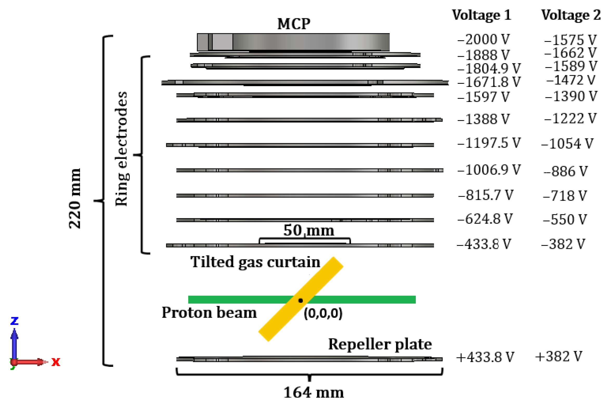
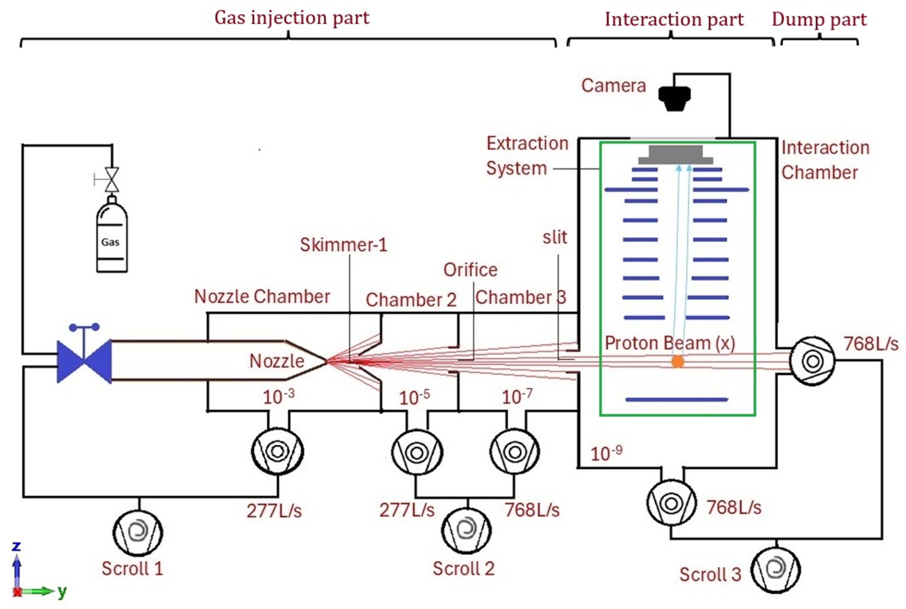
A novel beam monitoring technology, Supersonic Gas Curtain-based Ionization Profile Monitor (SGC-IPM), shown in Figure 1 capable of beam profile monitoring for charged particle beam, was initially developed at the Cockcroft Institute by the Quasar Group [20] and is being optimized for medical accelerators [21,22]. The SGC-IPM comprises the gas injection part, interaction part, and dump part. The injection part is capable of creating a supersonic gas jet, which is later introduced into the interaction chamber via a slit skimmer, oriented at 45° with respect to the gas jet direction. This will form a thin gas curtain, inclined at 45° with respect to the direction of the gas jet. In the interaction part, the incident beam ionizes the gas molecules of the gas curtain, the ions are then extracted with the extraction system composed of several electrodes and a MCP–phosphor screen assembly, and are captured with the help of a CMOS camera. The dump part includes a turbo molecular pump, to pump out the gas jet immediately after the interaction chamber, in order to avoid any impact on the background vacuum condition. The performance of the SGC-IPM is characterized using proton beams with the energy ranging from 4 MeV to 28 MeV with different beam currents from 1 to 100 nA at the MC40 Cyclotron Facility (University of Birmingham) and at the Dalton Cumbria Facility, Whitehaven in the United Kingdom [22]. This study indicates that the SGC IPM has the potential for real-time measurement of FLASH protons after further optimization.

In this study, the simulation of the extraction system of the SGC IPM is performed for a FLASH proton beam to verify its performance as a beam position and profile monitor. The simulations were performed in the CST studio suite [23] using a particle tracking solver and were benchmarked to the experimental results of the proton beam with a voltage of 28 MeV and a beam current of 70 nA. Various parameters affecting the profile reconstruction were discussed by Tzoganis V et al. in [20], such as camera resolution; MCP resolution; image broadening due to the gas jet curtain thickness; thermal velocity spread-induced image broadening; distortion caused by the space charge of the projectile beam; and a nonlinear external field. When it comes to the application in medical accelerators, where the beam size will depend on the tumor size, it is crucial to study the effect of different beam sizes on the beam profile and position measurement. The simulation results discussed in this work address this problem by studying the effect of different beam sizes on the profile measurement. Beam position monitoring using the extraction system, which is not explored before, is another important highlight of this work. Accounting for these two aspects in addition to the parameters and ideas explored in [20,22] will help to facilitate the clinical translation of the SGC-IPM as a unique solution for beam diagnostics for medical accelerators.

2. Methodology

The schematic of the SGC-IPM is given in Figure 1 where the interaction part houses the extraction system comprising a few ring electrodes, a repeller plate, and MCP. Electrostatic and particle tracking simulations were performed with the CST studio suite for the extraction system with proton beams of different beam sizes with practically possible potential conditions; this voltage configuration can be referred to as Voltage 1. Another set of simulations was performed to validate the beam profiles measured for the proton beam of 28 MeV energy and 70 nA beam current. Here the bias potentials of each plate and the MCP are slightly varied since we used a practical solution with two power supplies having two outputs each, where one output is fed into a voltage divider setup to distribute the potential across the plates, and the rest of the outputs were directly fed to the repeller plate, MCP, and phosphor screen. This potential configuration can be called Voltage 2. The details of the simulations carried out are explained in Section 2.1. The experimental studies with a 28 MeV proton beam having a 70 nA beam current are discussed in Section 2.2.

2.1. Simulation Studies of the Extraction System

The extraction system was modeled in CST with the bias voltages calculated for each ring electrode and repeller plate considering the voltage at the interaction point as 0 V and at the MCP as −2 kV. The voltage configuration, Voltage 1, is given in Figure 2, along with the dimensions of the extraction system, with (0, 0, 0) representing the center of the interaction region. In this study, the direction of the proton beam is considered along the X axis, the gas jet direction along the Y-axis, and the direction of extraction along the Z-axis. The crucial part of the simulation is creating the ion distribution considering the incident beam parameters, and the thickness and density of the gas curtain. A 100 MeV circular proton beam with a current of 600 nA and a Gaussian spatial distribution was considered for the simulation, as shown in Figure 3. This energy and beam current are relevant parameters for clinical FLASH protons [9]. A uniform density distribution of the gas curtain is assumed for the simulation and is modeled as a 1 mm thick planar sheet with uniform density of $3.9\times {10}^{16}$, particles/m³, which is measured using methods employed in the study within our group, presented in [24] and based on the studies reported in our earlier work [25].

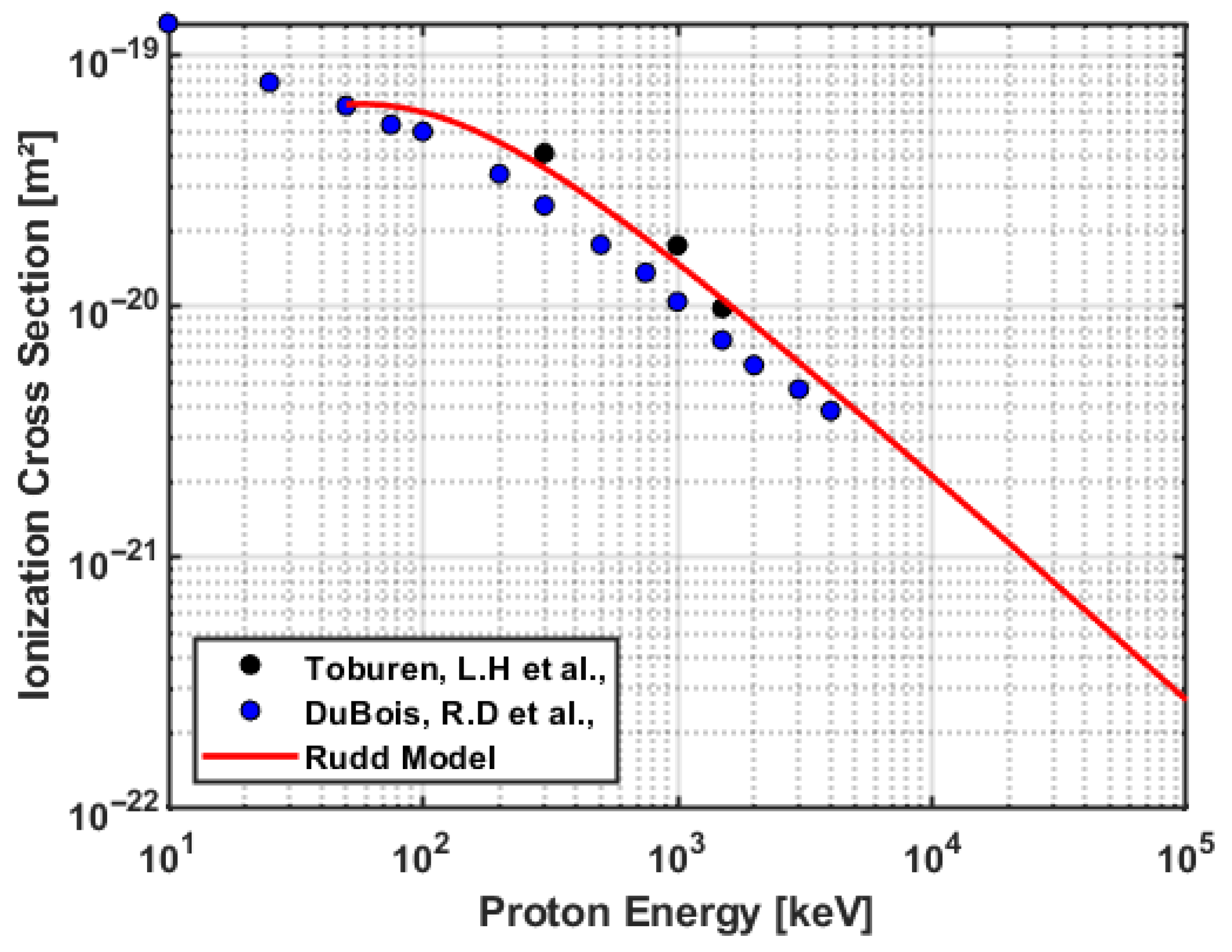
The next parameter that is to be considered for the simulation is the number of ions produced by the interaction of the proton beam with the gas curtain. The semi-empirical model proposed by Rudd et al. [26] was developed to describe total ionization cross-sections for proton impact on various gases, including argon, over a wide energy range (5–4000 keV). The model expresses the ionization cross-section as a sum over atomic subshells, each characterized by its binding energy $I_i$ and number of electrons $N_i$, with the energy dependence captured through the fitted parameters ${\sigma }_0$, A, B, C, and D:

$$\sigma =A{\sigma }_0\sum _i{N}_i{I}_i^{-2}{x}_i^B{\displaystyle \frac{ln(1+D{x}_i)}{C+x_i^{A+1}}},x_i={\displaystyle \frac{T}{I_i}},$$

(1)

where $T=E/m_p{m}_e^{-1}\approx E/1836$ represents the proton energy in electron units and E is the proton energy (eV). For argon, Rudd et al. determined $A=0.474$, $B=0.291$, $C=2.72$, and $D=94.4$, with an average deviation below 11% and ${\sigma }_0=6.51\times {10}^{-18}{\mathrm{m}}^2{\mathrm{eV}}^2$. This formulation reproduces the correct asymptotic limits, approaching the Bethe $E^{-1}lnE$ dependence at high energies and the $E^{1/2}$ scaling at low energies. In the present work, this model is employed to calculate the proton–argon ionization cross-section. The cross-section values calculated using the Rudd model exceed the experimental measurements by approximately 10–20%. The ionization cross-section is calculated using this model for proton energy up to 100 MeV. The experimental ionization cross-sections [27,28] up to 5 MeV available in the literature was used to cross-check the theoretical model. Based on this model, the number of ions ($2.84\times {10}^3$) produced for a proton beam of 100 MeV and 600 nA, for the given gas jet parameters, are then considered for the simulation. The extrapolation of the cross-section up to 100 MeV is shown in Figure 4.

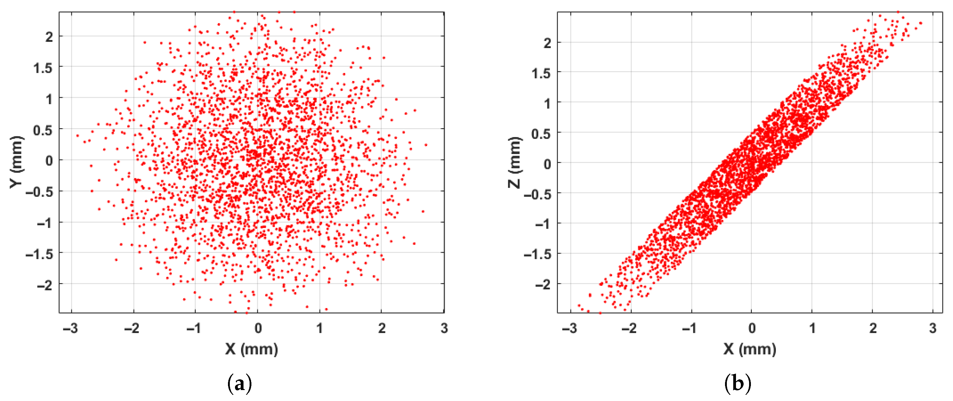
Given the 1 mm thickness of the gas curtain, the Gaussian proton beam with radius b generates a three-dimensional interaction region rather than a purely two-dimensional projection. When intersecting the curtain tilted at $45$°, the beam’s transverse Gaussian profile appears as a distorted circle with an elongated side $a=b/sin(45°)$ along the tilt. 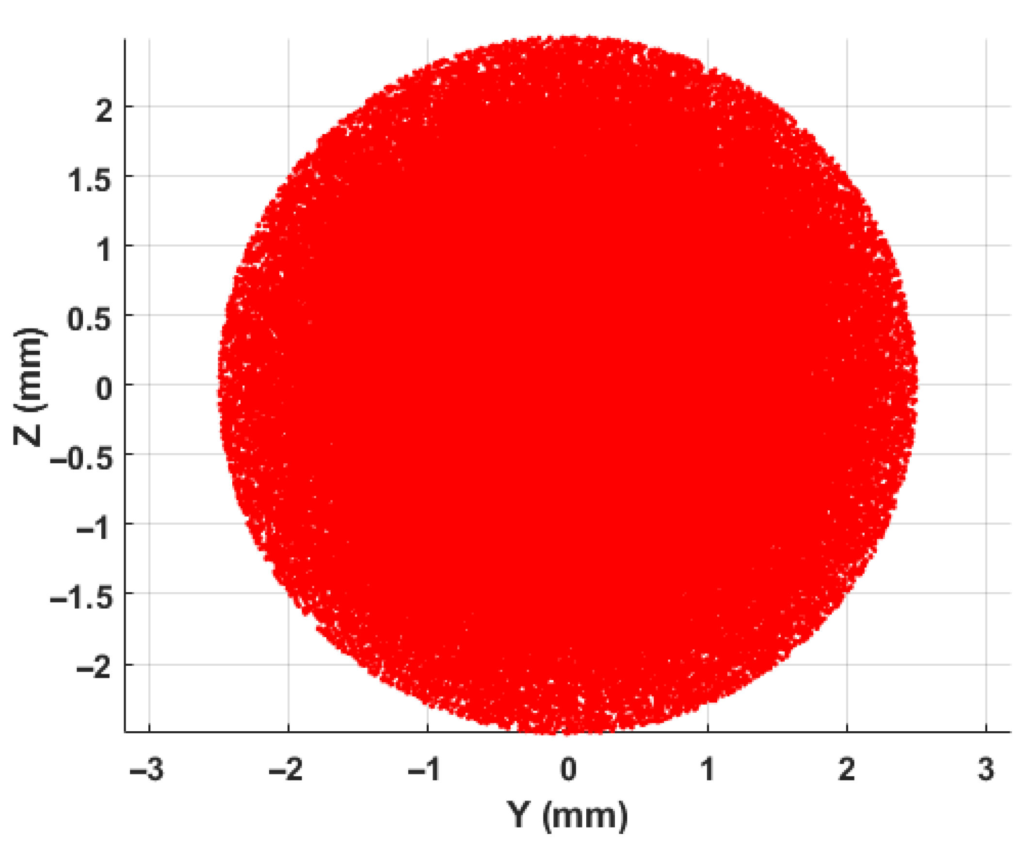Consequently, the ion distribution occupies a 1 mm thick volume normal to the curtain plane and exhibits an elliptically elongated shape consistent with the projected beam width b and the curtain orientation. The total ions thus calculated using the Rudd model are assigned a Gaussian distribution inside this volume. This distribution of particles represents the spatial density of ionized gas in the interaction region. In the detector perspective, the effect of the tilt will be canceled out as it will see the XY projection of this distribution. Figure 5 illustrates the resulting particle distribution projected in the XY plane and in the XZ plane, respectively, for a proton beam with a radius of 2.5 mm, highlighting the circular projection and spread along the X-direction, induced by the curtain thickness.

Each ion was assigned an initial terminal velocity of 587 m/s in the Y-direction, corresponding to the supersonic gas flow, where the gas is injected with 5 bar injection pressure at room temperature. The final dataset of the ion interface includes spatial coordinates, momentum vectors to include the velocity component, and intrinsic ion properties such as mass and charge. The momentum component in the rest of the directions was considered zero as the gas jet does not have any significant velocity components along these directions [24].

The ion trajectories were simulated using the particle tracking solver within CST Studio Suite. The input distribution, generated externally, was imported as the initial condition and electrostatic fields generated by the plates were considered in the simulation. The position and energy of ions were measured using a 2D particle monitor positioned near the MCP, in the drift region, through which the ions travel towards the MCP, to get the spatial and energy information of the particles passing though this monitor, which further provides information on the transverse beam profile, ion energy distribution, and spatial density at the detection plane. The ion profile recorded at the MCP plane is directly representative of the signal from the MCP expected on the upstream CMOS camera. The simulation is repeated for five beam radii of 0.5 mm , 2.5 mm, 5 mm, 10 mm, and 15 mm.

An additional set of simulation data with position offsets of ±1 mm and ±5 mm in Y and Z directions with reference to the interaction point for the incident proton beam was taken. These offsets represent position changes of the incident proton beam in the vertical (up/down) or horizontal (left/right) directions. The gas curtain will act as a screen for the proton beam, which will track any position changes of the proton beam hitting the screen. Consequently, the ion interface will have the corresponding position changes and this will be extracted further towards the MCP. For each beam shift, corresponding displacement in the centroid of the ion distribution at the MCP, with respect to the beam–gas curtain interaction point, is quantified. Ideally, the center of the MCP–phosphor screen assembly coincides with the interaction point, which will make it easy to measure the shift in the experimental scenarios.

2.1.1. Reconstruction of Beam Profile

For a uniform electric field distribution across the drift region, the true distribution of the proton beam is determined after the MCP is affected by several factors including the ones listed in the study by Tzoganis. V et al. in [20]. The current simulation accounts for the factors introduced by the gas curtain thickness, ionization, and the detection efficiency of the MCP. The incident proton beam can be considered as a function A(y, z) with n number of particles having Gaussian distribution. After interacting with the gas curtain, it undergoes transformation based on two factors such as the gas curtain thickness, T(x), and the number of ions $N\left(\sigma \left(E_{\mathrm{proton}}\right)\right)$ produced, where $E_{\mathrm{proton}}$ is the incident proton energy. The effect of ionization is straight forward without affecting the Gaussian distribution, but the thickness will have a greater impact on smaller beams with radii in the order of a few mms, and will reduce as the beam size increases, as the thickness becomes insignificant compared to the beam size. The next parameter is the detection efficiency of the MCP, Q(E), which depends on the energy, E, of each ion impinging on the MCP. Based on these factors, the final projected beam profile, O(x,y), after the MCP will be different with respect to the incident beam profile.

$$O(x,y)=N\left(\sigma \left(E_{proton}\right)\right)·Q\left(E\right)·G·A(y,z)+T\left(x\right)$$

(2)

The projected beam profile is reconstructed from simulation data consisting of x, y, and E, where x and y represent transverse positions and E is the corresponding particle energy. A two-dimensional spatial energy map is generated with this data. This spatial distribution of ions is weighted according to the energy-dependent detection efficiency of the MCP. Each particle’s contribution was scaled by the corresponding efficiency data taken from [29]. To simulate the finite resolution of the MCP, the weighted positions are bound according to the $25\mu \mathrm{m}$ channel size, generating a 2D map of normalized detected counts. The X and Y profiles are extracted from this distribution and Gaussian fits are applied to quantify the beam widths. This approach allows for visualization of the combined effects of the gas curtain thickness and energy-dependent detection efficiency on the measured beam profile. The true beam profile distribution can be obtained by reversely applying these impact factors by quantifying each.

2.2. Proton Beam Profile Measurement

Beam profile measurements were conducted by capturing the signal produced by the ions from the MCP–phosphor screen assembly on a CMOS camera [22]. A voltage divider set up was used to uniformly distribute the voltages across the plates from a single power supply unit, where the positive voltage was given to the repeller plate. MCP-phosphor screen assembly was biased with an additional power supply unit. The MCP was biased at −2.1 kV with an external power supply, and additionally a current-limiting resistor is connected in series with the MCP input. This causes a voltage drop across the resistor by which the actual voltage on the MCP is lower than the power supply output. The MCP therefore operates at this reduced voltage of −1.575 kV. The MCP is coupled to a phosphor screen, which is set to a positive potential of 3 kV, to convert the ion impacts into a visible light signal, which will represent the projected beam profile of the incident proton beam. During the experiment, two of the ring electrodes were shortened due to the vibrations from the transport, which was accounted for in the simulations conducted for the experimental conditions.

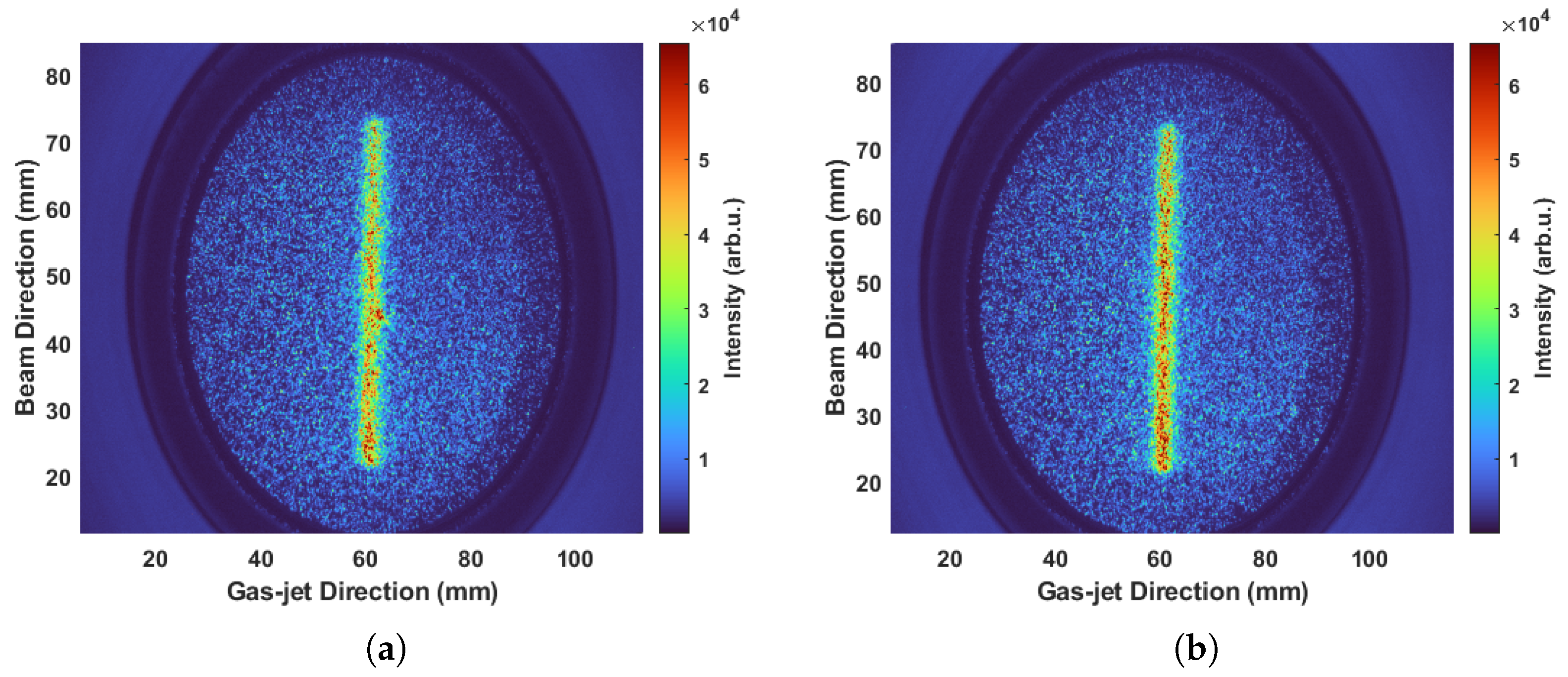
The camera was setup in a way that it ensures the capturing of the phosphor screen and the camera gain was set to a value of 240 to ensure a high dynamic range and to avoid signal saturation. The images were captured for different exposure times from 200 ms to 750 ms. The background image was acquired with the gas curtain turned off and subtracted from the image that is captured while the gas jet was turned on to suppress the contribution of beam-induced background ionization. The resulting 2D image represents the transverse profile distribution of the proton beam as mapped by the ion interface. Both the images with the gas jet on and off are given in Figure 6a,b; these images were used to reconstruct the vertical and horizontal beam profiles. Following this method, the beam profiles were measured for the 28 MeV proton beam with a 70 nA beam current.

As mentioned earlier in Section 2.1, the ions generated in the interaction region drift in the direction of the gas flow as they are extracted from this region. In contrast, ions produced by beam-induced background processes do not exhibit this drift during extraction. Consequently, the signal from the gas curtain ions shows a slight spatial offset relative to that from the beam-induced background ions as in Figure 6a. Although this offset is present for all beam sizes, it becomes more pronounced for smaller beams. When the beam size is smaller than the displacement caused by the drift, this effect aids in separating the image formed by the gas curtain ions from that produced by beam-induced background ionization. Because no independent measurement of the beam size was recorded during the experiment, the beam-size input for the CST simulation could not be constrained, and a direct comparison of the simulated and experimental beam profiles was therefore not possible. Instead, the drift-induced offset provides a beam size-independent observable for comparison. This drift will depend on the terminal velocity of the gas curtain and remains the same irrespective of the proton beam parameters. The simulations were performed for the experimental parameters and the shift in the center of the transverse beam profile and the diffused line due to the background were quantified and compared for both cases. The vertical and horizontal profiles were reconstructed using CST simulations with the experimental conditions. The shift observed in the experimental beam profiles and the simulation results were compared to validate the design and potential configuration of the extraction system and the effect of the directional velocity of the gas jet molecules.

3. Results and Discussion

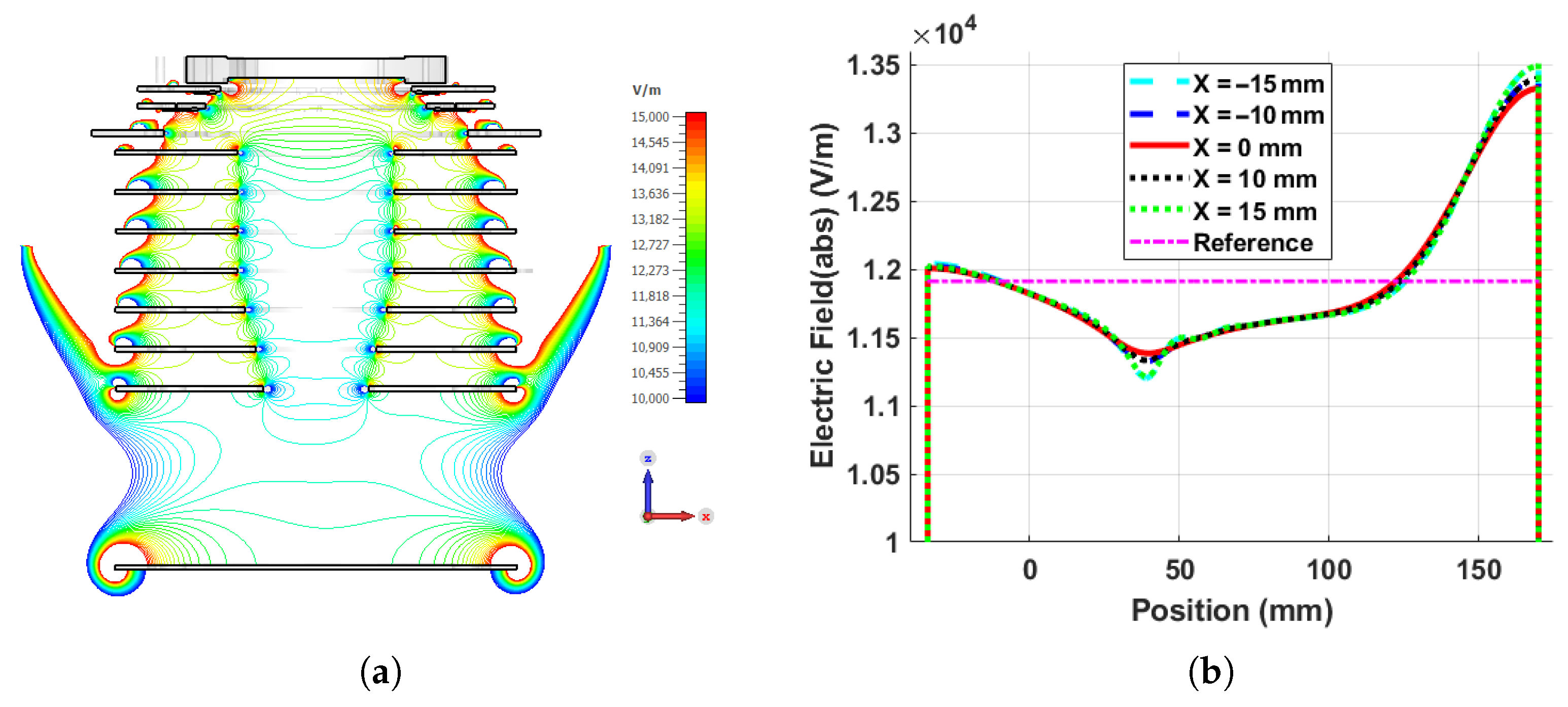
The simulated electric field distribution due to the Voltage 1 setup, along the drift region, through which the produced ions travel to the MCP, is shown in Figure 7a,b. A 1-D distribution of absolute electric field component in the drift region is shown along the center of the X-axis and at ±10 mm and ±15 mm offsets. Since the distribution is symmetrical around the drift region and corresponds to (X, Y) = (0, 0), the electric field distribution will be same for the Y offsets as well, which in turn shows the uniform ion trajectory throughout the extraction. The 1D distribution of the Z-component of the electric field presented in the figure ensures the minimally distorted spatial distribution of the ions throughout the extraction. A maximum inhomogeneity of ±11.87% relative to the mean value of the electric field along the drift region for X = 0 mm was found in the electric field. The error introduced by this field variation in the X and Y profiles was found to be ±3% for all the beam sizes considered.

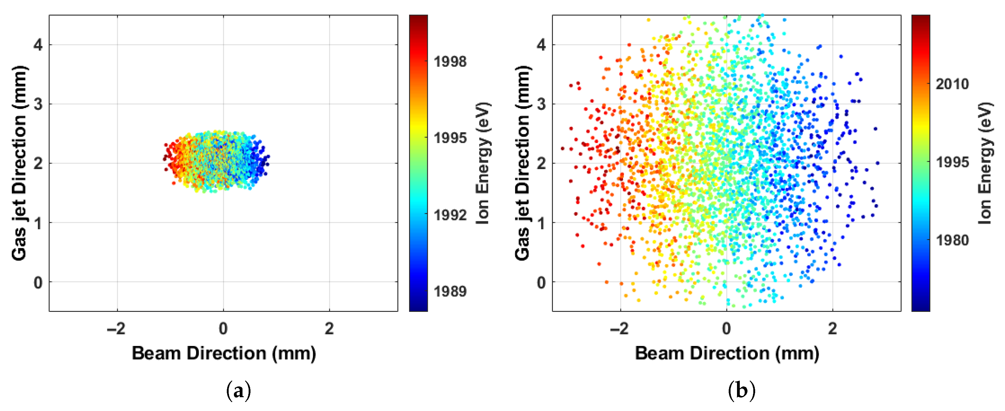
The spatial energy distributions of the ions accelerated towards the MCP through this uniform electric field are monitored before and after extraction. A non-uniform energy distribution was found for the ions reaching the MCP as expected because of the varying travel distance of the ions from the interaction points on the gas curtain due to the 45 degree inclination. Ions originating from the lower end of the tilted curtain travel a greater distance and consequently acquire higher energy upon reaching the MCP compared to ions created from the upper end of the curtain.

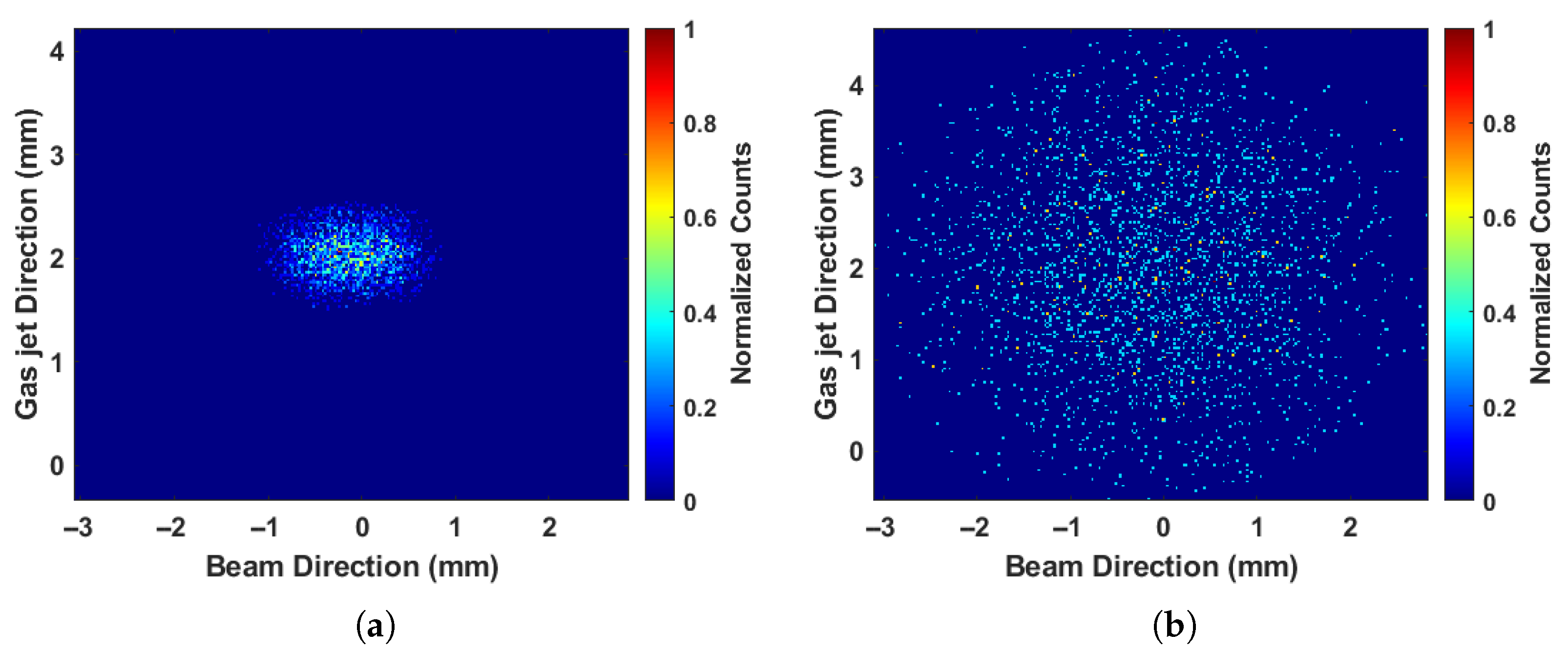
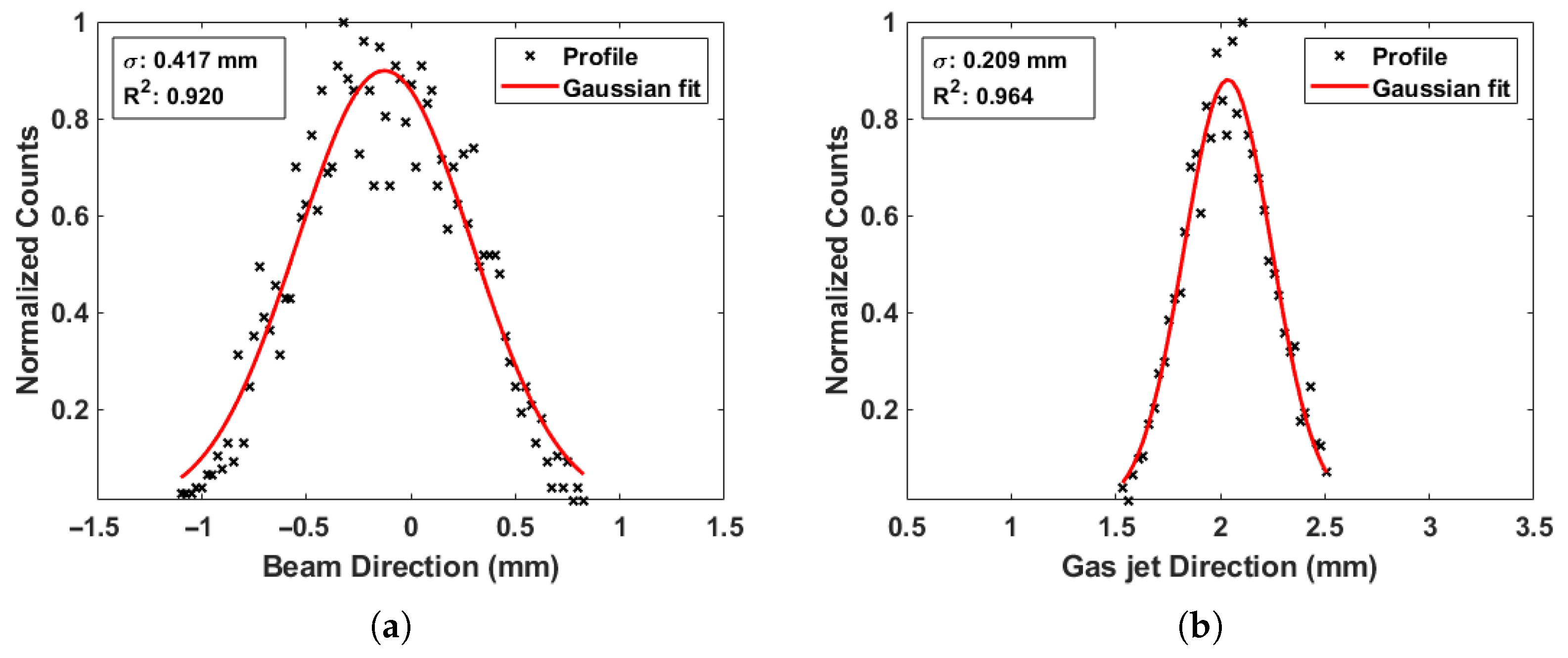
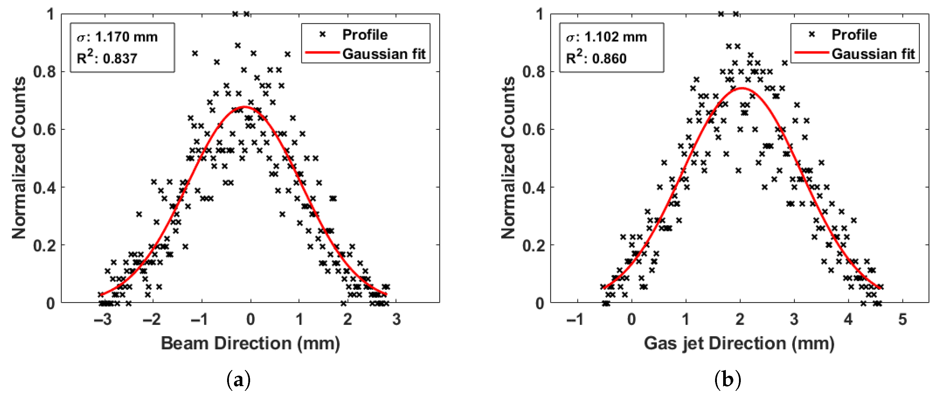
The two-dimensional spatial energy map of the ions generated for the incident proton beam radii of 0.5 mm (FWHM_y = 0.485 ± 0.013 mm, FWHM_z = 0.483 ± 0.012 mm) and 2.5 mm (FWHM_y = 2.420 ± 0.009 mm, FWHM_z = 2.412 ± 0.009 mm) are given in Figure 8a and Figure 8b, respectively. The resulting normalized distributions after introducing the detection efficiency are shown in Figure 9a,b for proton beam radii of 0.5 mm and 2.5 mm, respectively. The vertical and horizontal profiles were extracted from this distribution and Gaussian fits were applied to quantify the beam widths. The reconstructed beam profiles for 0.5 mm and 2.5 mm beam radii are shown in Figure 10 and Figure 11, respectively. The results reveal that the Y profile remains less distorted, reflecting the intrinsic gas curtain thickness, while the X profile is broadened, consistent with spatial distortion along that axis. The corresponding measured beam FWHMs were 0.982 ± 0.0751 mm (vertical) and 0.493 ± 0.0706 mm (horizontal) for the 0.5 mm beam, and 2.755 ± 0.0047 mm (vertical) and 2.595 ± 0.0039 mm (horizontal) for the 2.5 mm beam. The large deviation in the X profile of 0.5 mm beam is due to the 1 mm thickness of the gas curtain, which is significant compared to the beam radius, but for the 2.5 mm beam where the gas curtain thickness is less than the beam radius, it has less of an impact.

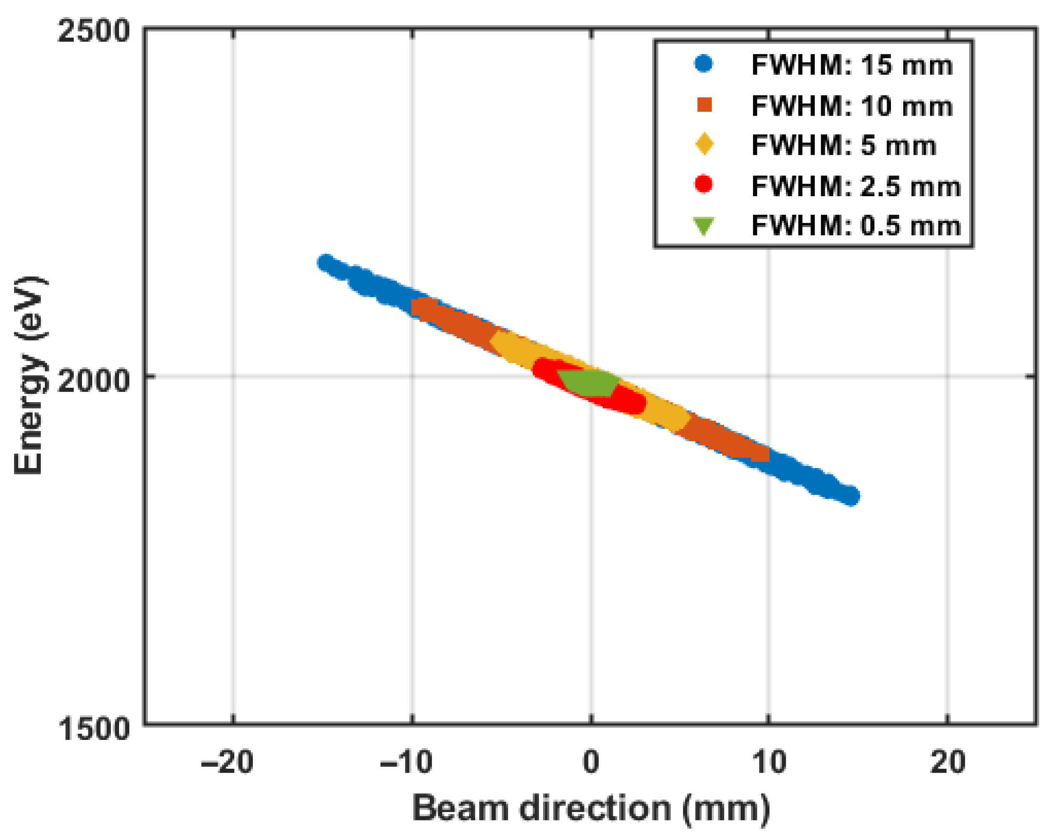
The evaluated energy distributions for the beams with radii of 0.5 mm, 2.5 mm, 5 mm, 10 mm, and 15 mm are given in Figure 12. The inhomogeneity in each case is quantified as the deviation from the average value of the energies and was found to be ±0.29%, ±1.42%, ±2.90%, ±5.45%, and ±8.48% for 1 mm, 5 mm, 10 mm, 20 mm, and 30 mm beams, respectively. This inhomogeneity will naturally increase as the beam size increases and is negligible for the beam with the 0.5 mm radius, as there will not be a significant effect in the detection efficiency of the MCP for ions with 1.9 keV to 2.1 keV [29,30]. The increased inhomogeneity for the larger beam sizes can further result in a distorted beam profile due to the distortion in the signal from MCP caused by the varied detection efficiency, which further effects the reconstruction of the beam profile from the phosphor screen images. This should be resolved to obtain the true beam profile distribution, as discussed in Section 2.1.1. This inhomogeneity does not affect the beam profile reconstruction in the Y-axis, since for a single X-component, the energy of the ions along the Y-axis was constant, as shown in Figure 8.

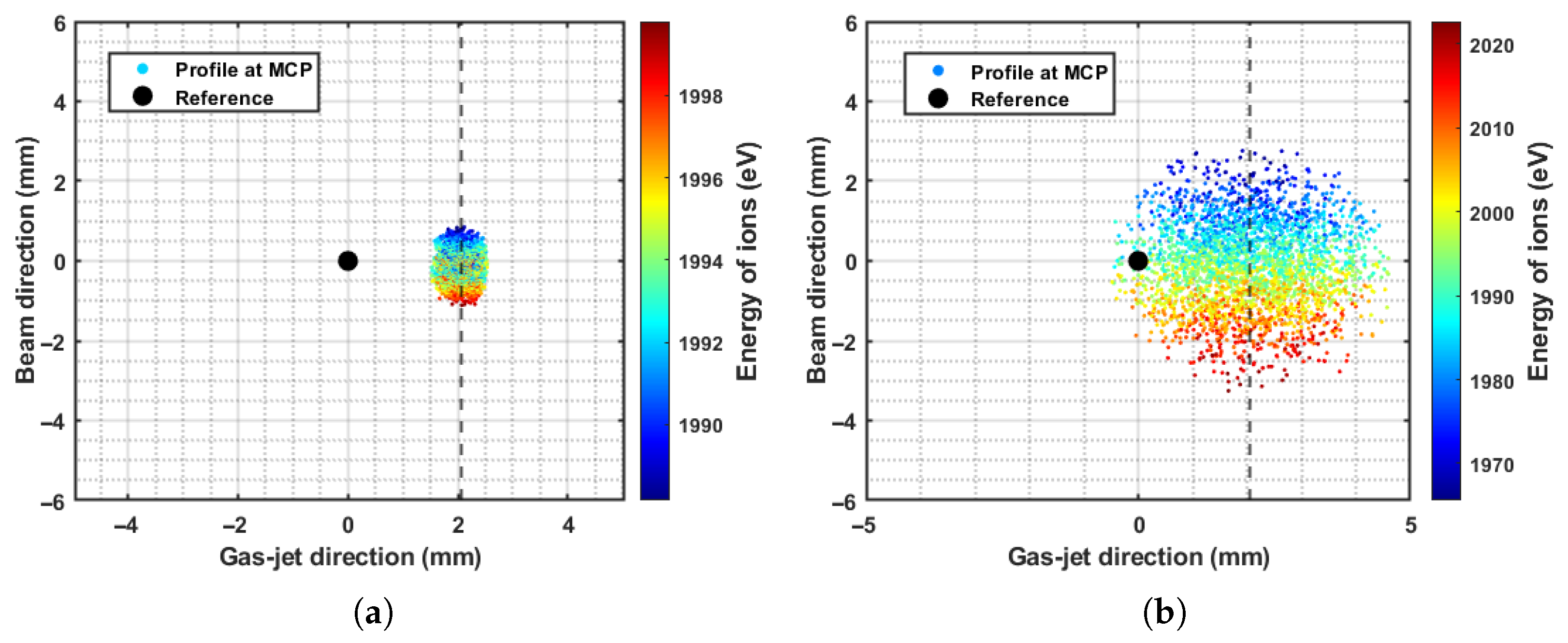
Another observation in the simulation, with the Voltage 1 setting, is the shift of 2.05 mm in the centroid of the spatial distribution of the ions, and further on the beam profile, from the central axis of the extraction system along the Y-direction. This shift helps to differentiate the beam profile due to the gas jet from that resulting from the background, regardless of the intensity difference between these two profile distributions. The shift is visible when it is comparable to the beam size, as given in Figure 13, for the 0.5 mm and 2.5 mm beam radii. As the beam sizes are increased further, the transverse beam profile and the background tend to overlap with each other and will make it difficult to identify this shift. As this shift is solely resulting from the supersonic gas jet flow, it is the same for all the other higher beam sizes as long as the gas jet properties are the same.

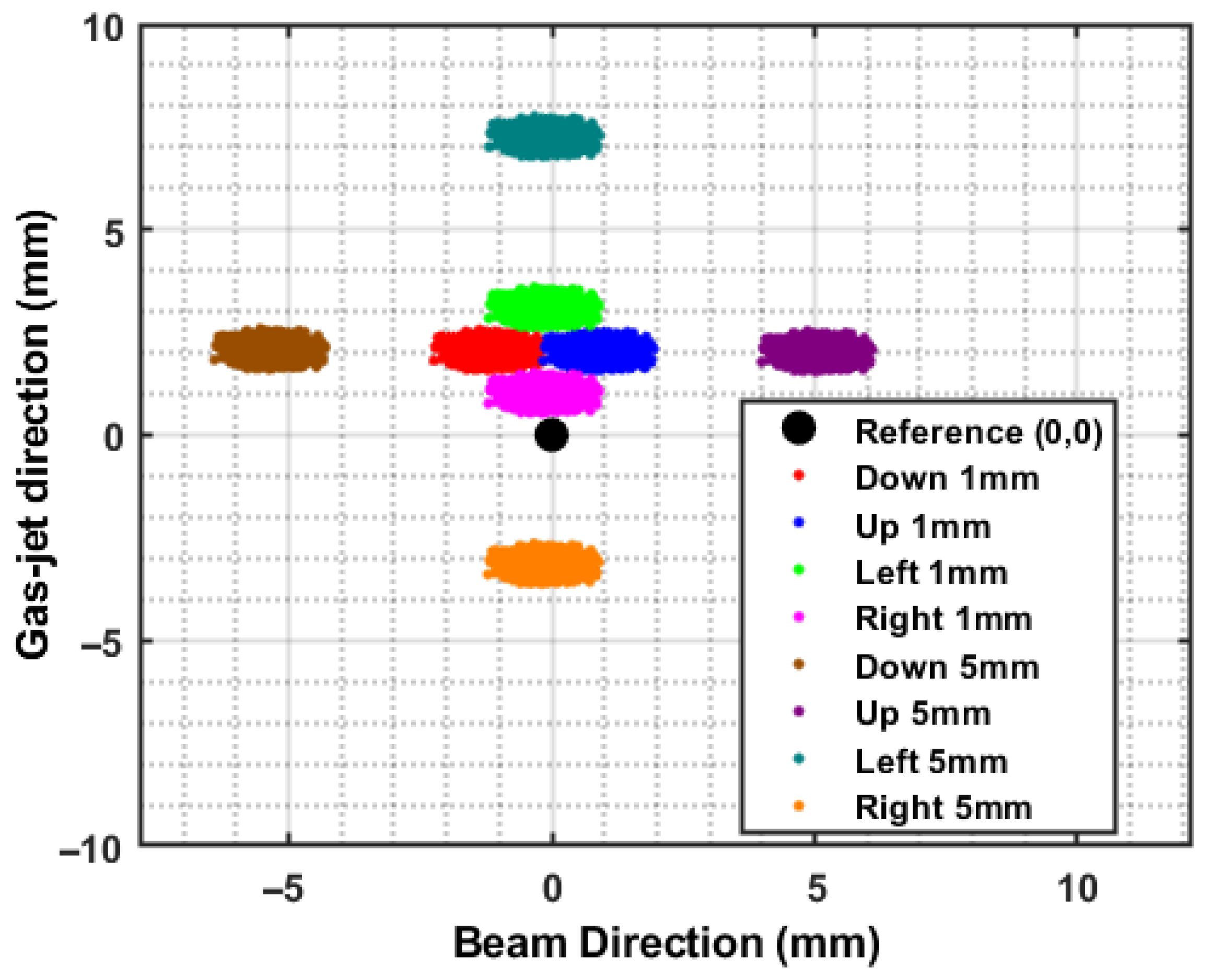
The simulations conducted to verify the beam position monitoring showed successful results, with the introduced offsets to the proton beam proportionally reflected in the beam profile measurements at the MCP. For the applied beam shifts of 1 mm and 5 mm, relative to the interaction region reference (0, 0, 0), in both the vertical (up/down) and horizontal (left/right) directions, the corresponding deviations of the beam profile centroid from the MCP center were quantified and are presented in Figure 14. Here, the interaction region reference $(0,0,0)$ and the geometric center of the MCP lie along the ion extraction axis. The MCP is positioned at $Z=Z_{\mathrm{MCP}}$, and measurements are performed in the transverse $(X,Y)$ plane relative to the MCP center $(X,Y)=(0,0)$. This allows for beam profile deviations at the detector to be quantified with respect to the interaction region reference. The linear response in the beam profile with the proton beam offsets supports the performance of the IPM for beam position monitoring. In the present extraction geometry, the measurable beam position range is constrained by three factors: (i) the projected height of the tilted gas curtain, (ii) the 50 mm inner diameter of the ring electrodes, and (iii) the transverse beam size. For a gas curtain of physical height h tilted by 45°, the effective height seen by the detector is $h_{\mathrm{gas}}=h/\sin 45°$ (projected gas curtain width), and this projected height must remain within the electrode aperture, i.e. $h_{\mathrm{gas}}\le 50\mathrm{mm}$. Denoting the electrode aperture by $D=50\mathrm{mm}$ (ring electrode inner diameter) and the beam radii in the x- and y-directions at the interaction point by $b_x$ and $b_y$, the measurable position ranges are $\Delta x_{\mathrm{mon}}=min(h_{\mathrm{gas}},D,b_x)$ (monitorable horizontal range) and $\Delta y_{\mathrm{mon}}=min(h_{\mathrm{gas}},D,b_y)$ (monitorable vertical range). Because the ion signal at the MCP is shifted by $\Delta y_0=2.05\mathrm{mm}$, due to the terminal velocity of the ionized gas particles, the accessible position monitoring window at the MCP becomes $x\in [-\Delta x_{\mathrm{mon}}/2,\Delta x_{\mathrm{mon}}/2]$ for horizontal monitoring and $y\in [-(\Delta y_{\mathrm{mon}}/2-\Delta y_0),\Delta y_{\mathrm{mon}}/2-\Delta y_0]$ for vertical monitoring. For example, a narrow beam (e.g., $b_x=b_y=1\mathrm{mm}$) can be displaced by almost the full electrode radius (±25 mm) while remaining detectable. However, for a wider beam (e.g., $b_x=b_y=15\mathrm{mm}$), the detectable offset range is smaller, since part of the ionization region reaches the acceptance limit sooner. The reference (0, 0) at the MCP can be marked at the geometrical center of the MCP. The extraction system can be calibrated using a reference measurement using any other established measurements such as scintillator screens or films.

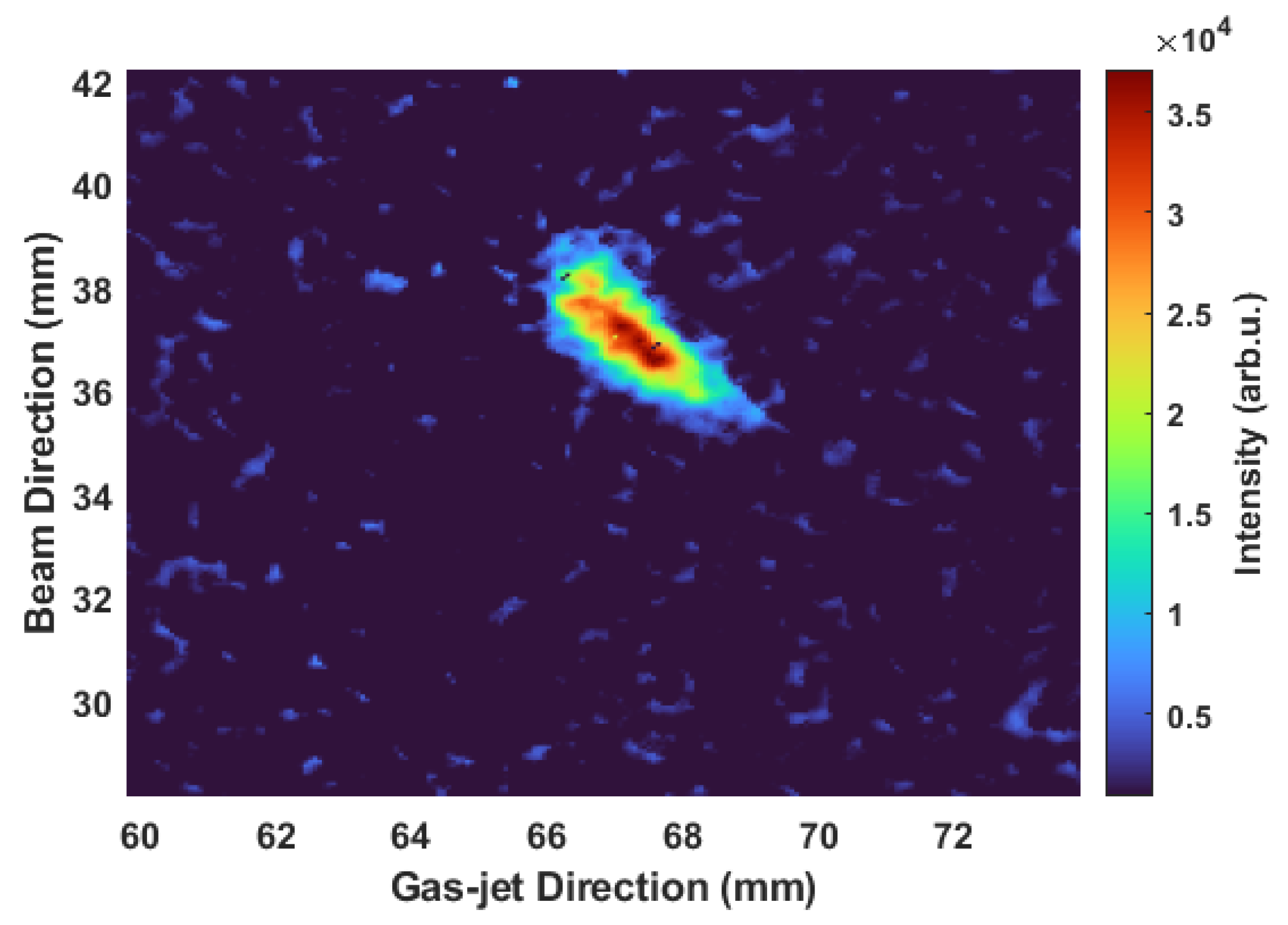
The 2D transverse intensity distribution of the beam, as captured by the CMOS camera, was further analyzed to extract its horizontal and vertical profiles. Figure 15 and Figure 16 present the measured 2D transverse distribution and its corresponding horizontal and vertical projections, respectively, which are reconstructed from the mean of 20 images of the phosphor screen with gas jet on and off conditions. A pixel-to-millimeter conversion factor of 0.07035 ± 0.002 mm/pixel was established for the experimental setup based on the distance of the camera from the MCP–phosphor screen assembly and the focal length of the camera, enabling the conversion of all pixel-based measurements into physical units. The beam profiles were recorded with an integration time of 500 ms for the 28 MeV proton beam at a beam current of 70 nA.

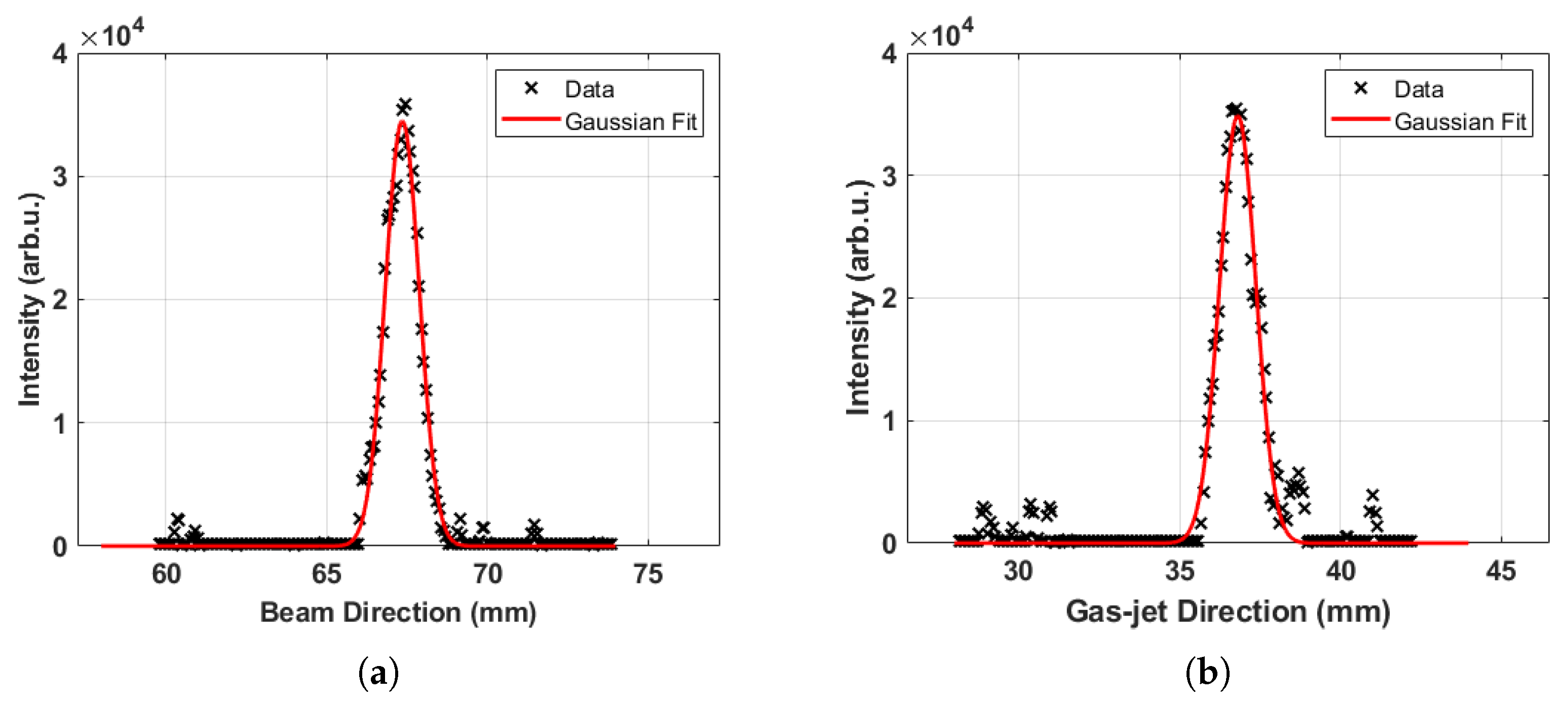
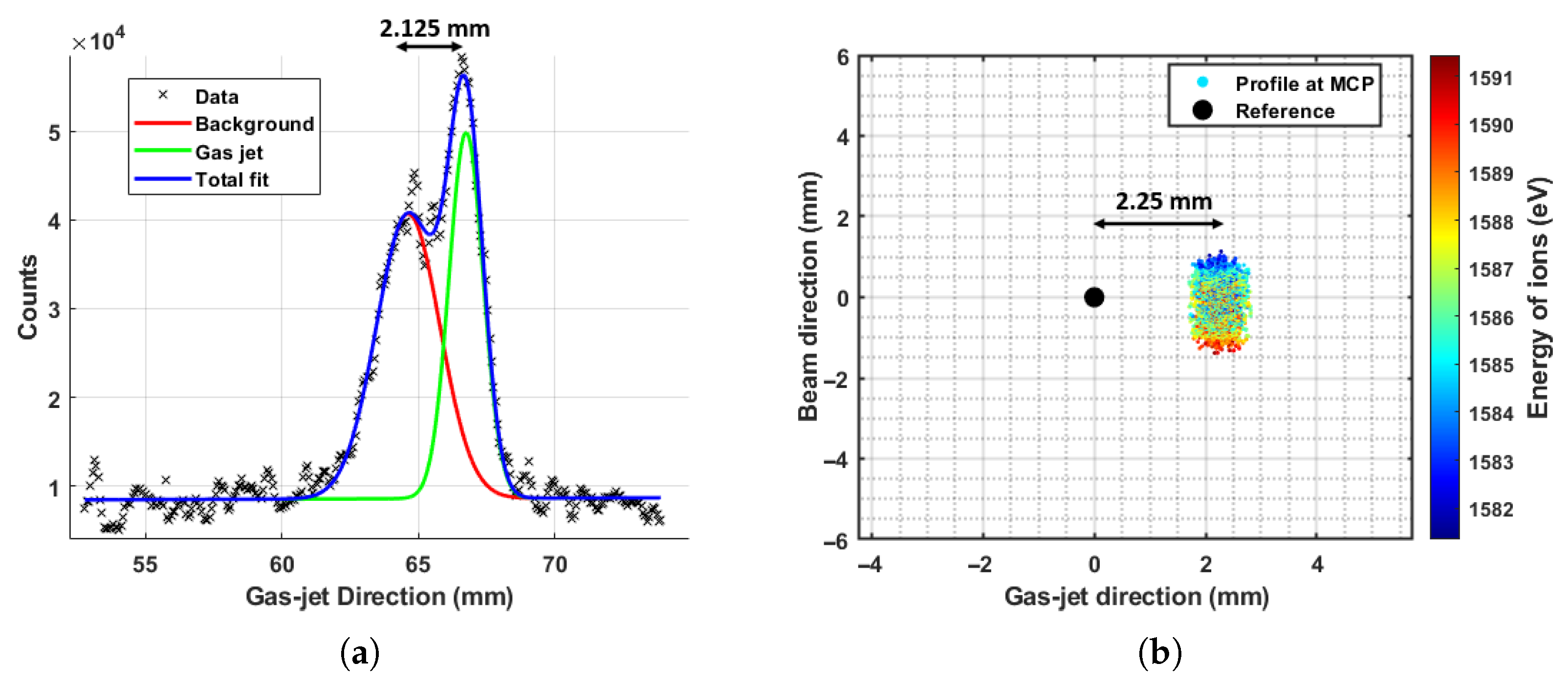
To quantify the shift in the experimental transverse profile induced by the directional velocity of the gas jet particles, a one-dimensional intensity distribution was extracted along a line intersecting both the diffused background beam profile and the localized gas jet-induced profile within the 2D spatial distribution. The extracted 1D distribution, presented in Figure 17, clearly reveals two distinct peaks corresponding to the background and gas jet profiles. The center of the background peak corresponds to interaction region reference (0, 0, 0). The separation between the Gaussian fits of the peaks is measured to be approximately 2.125 mm. This experimental result was compared with the simulation output, which was 2.25 mm, with the voltage setting, Voltage 2, while also accounting for the shorted plates. The minor deviation between the measured and simulated shifts primarily results in uncertainties in the gas molecules’ terminal velocity, which is sensitive to temperature uncertainties. The good agreement between the quantified shifts in the simulation and measurement further validates the accuracy of the simulation in capturing the beam profile from beam–gas interactions.

4. Conclusions

In this work, we evaluated the performance of the extraction system of a Supersonic Gas Curtain Ionization Profile Monitor (SGC-IPM) for transverse beam profile and position measurements of clinically relevant proton beams. Using CST particle tracking simulations benchmarked against low-energy experimental data, we demonstrated that the SGC-IPM can reconstruct transverse beam profiles for the small beam sizes studied and exhibited a linear response to intentional beam position offsets, confirming its capability as a position-sensitive diagnostic. This study introduces two key advances beyond previous work on gas jet-based IPMs developed within our group. First, the extraction system provides reliable beam position monitoring, with reconstructed centroid shifts showing a highly linear correspondence to intentional beam offsets. Second, we note that for larger beam sizes, ion distribution inhomogeneity caused by the 45° curtain tilt could affect profile reconstruction. This observation highlights a potential limitation and guides considerations for future design optimization. While the lack of an independent beam size measurement prevented a direct comparison of experimental and simulated beam profiles, the drift observed in the simulation, caused by the terminal velocity of the gas jet, matched that seen in the measurements. This agreement indicates that the ion interface model captures the relevant gas jet dynamics. Building on these results, efforts are underway to develop a compact variant of the SGC-IPM, enabling seamless integration into compact medical accelerator systems, such as laser-driven accelerators.