Abstract
The analysis of level statistics provides a primary method to detect signatures of chaos in the quantum domain. However, for experiments with ion traps and cold atoms, the energy levels are not as easily accessible as the dynamics. In this work, we discuss how properties of the spectrum that are usually associated with chaos can be directly detected from the evolution of the number operator in the one-dimensional, noninteracting Aubry-André model. Both the quantity and the model are studied in experiments with cold atoms. We consider a single-particle and system sizes experimentally reachable. By varying the disorder strength within values below the critical point of the model, level statistics similar to those found in random matrix theory are obtained. Dynamically, these properties of the spectrum are manifested in the form of a dip below the equilibration point of the number operator. This feature emerges at times that are experimentally accessible. This work is a contribution to a special issue dedicated to Shmuel Fishman.
1. Introduction
There has been a surprising revival of interest in quantum chaos, especially from a dynamical perspective, with the exponential growth of out-of-time ordered correlators (OTOC) taken as a main indication of chaotic behavior [1,2,3,4,5,6,7,8,9]. The more traditional approach to quantum chaos, however, focuses on the properties of the spectrum and uses level statistics as in random matrix theory (RMT) as its main signature [10,11,12,13]. There are several examples of cases where a correspondence between the exponential growth of the OTOC and level repulsion as in RMT has been found [14,15,16,17,18], but exceptions also exist [19,20,21]. In the present work, we propose a way to directly detect the effects of level repulsion in the evolution of a quantum system. The quantity and model that we consider, namely, the number operator and the Aubry-André model, are accessible to experiments with cold atoms [22].
The Aubry-André model has quasiperiodic disorder [23,24,25,26,27], so is contrary to the Anderson model where the disorder is random, in one-dimension (1D), and for a single particle, it can present both localized and delocalized regimes. All states in the Aubry-André model become localized only above a critical disorder strength, while in the one-particle 1D infinite Anderson model, all states are localized for any disorder strength [28,29,30,31]. Despite this difference, when the systems are finite and have small disorder strengths, they present similar level spacing distributions; namely, they show distributions as in RMT, the so-called Wigner–Dyson distributions [32,33]. This is a finite-size effect, not a signature of chaos. Wigner–Dyson distributions in these non-chaotic 1D models emerge when the localization length is larger than the system size. However, these models can still be used as a way to demonstrate how the properties of the spectrum get manifested in the dynamics of realistic quantum systems. Here, we show how the level repulsion present in the finite one-particle 1D Aubry-André model affects its dynamics.
In studies of many-body quantum systems, it has been shown that the survival probability, that is, the probability to find the system in its initial state later in time, decays below its saturation value in systems that present level repulsion [34,35,36,37,38,39,40,41,42,43]. This dip below saturation is commonly known as correlation hole [34,35,36,37,38,39,40,41]. In many-body quantum systems, the time for its appearance grows exponentially with system size [44], which makes its experimental observation very challenging even for relatively small systems. To circumvent this issue, one could employ systems with few-degrees of freedom [33,45]. However, two other problems remain: the correlation hole in systems with many particles emerges at extremely low values of the survival probability, and this quantity is non-local in real space, while experiments usually deal with local quantities (exceptions include [46]).
To solve these problems, we consider the one-particle 1D Aubry-André model and study the evolution of the number operator. This is a local quantity routinely measured in experiments with cold atoms. In the presence of level repulsion, a correlation hole develops at times that grow just sublinearly with the system size. In addition, for systems that are not too large, the minimum point of the hole occurs at values that are not very small, and therefore, do not require extraordinary precision for detection. All these factors should make the experimental observation of the correlation hole viable in this model.
Before proceeding with the presentation of our results, we note that this work is a contribution to a special issue dedicated to Shmuel Fishman. As such, we find it pertinent to mention that Griniasty and Fishman studied a generalization of the Aubry-André model in [47]. We expect our results to be valid in this broader picture also.
2. Finite One-Particle One-Dimension Aubry-André Model
We study the one-particle 1D Aubry-André model with open boundaries described by the following Hamiltonian,
Above, is the creation (annihilation) operator on site j. The first term defines the quasiperiodic onsite energies with disorder strength h; is a phase offset chosen randomly from a uniform distribution ; the second term is responsible for hopping the particle along the chain (we choose ), and L is the number of sites.
The basis vectors that we use to write the Hamiltonian matrix correspond to states that have the particle placed on a single site j, such as . The eigenvalues of the matrix are denoted by and the corresponding eigenstates are , where .
2.1. Level Statistics
To study the degree of short-range correlations between the eigenvalues, we consider the level spacing distribution , which requires unfolding the spectrum [11,48], and the ratio between neighboring levels [49,50], which does not require unfolding the spectrum. To detect long-range correlations, we look at the level number variance [11,48], which also requires unfolding the spectrum.
The unfolding procedure consists of locally rescaling the energies. The number of levels with energy less than or equal to a certain value E is given by the staircase function , where is the unit step function. has a smooth part , which is the cumulative mean level density, and a fluctuating part . By unfolding the spectrum, one maps the energies onto , where , so that the mean level density of the new energy sequence becomes one. Statistics that measure long-range correlations are more sensitive to the unfolding procedure than short-range correlations [51]. In this paper, we discard 20% of the energies from the edges of the spectrum, and obtain by fitting the staircase function with a polynomial of degree 7.
2.1.1. Short-Range Correlations
In the spectra of full random matrices, neighboring levels repel each other and follows the Wigner–Dyson distribution. The exact form of the distribution depends on the symmetries of the Hamiltonian.
has for the Gaussian orthogonal ensemble (GOE), where the full random matrices are real and symmetric; for the Gaussian unitary ensemble (GUE), where the full random matrices are Hermitian; and for the Gaussian symplectic ensemble (GSE), where the full random matrices are written in terms of quaternions. The values of the constants for and are found, for example, in [48]. The degree of correlation between the eigenvalues increases from GOE to GUE to GSE.
In contrast with the spectra of RMT, one may find systems with uncorrelated eigenvalues, where the level spacing distribution is Poissonian and systems with eigenvalues that are more correlated than in random matrices and nearly equidistant, as in the "picket-fence"-kind of spectra [52,53] and the Shnirelman’s peak [54].
The ratio between neighboring levels is defined as [49,50]
and is the spacing between neighboring levels. The average value over all eigenvalues varies as follows: for the Poissonian distribution, for the GOE, for the GUE, for the GSE, and for picket-fence-like spectra.
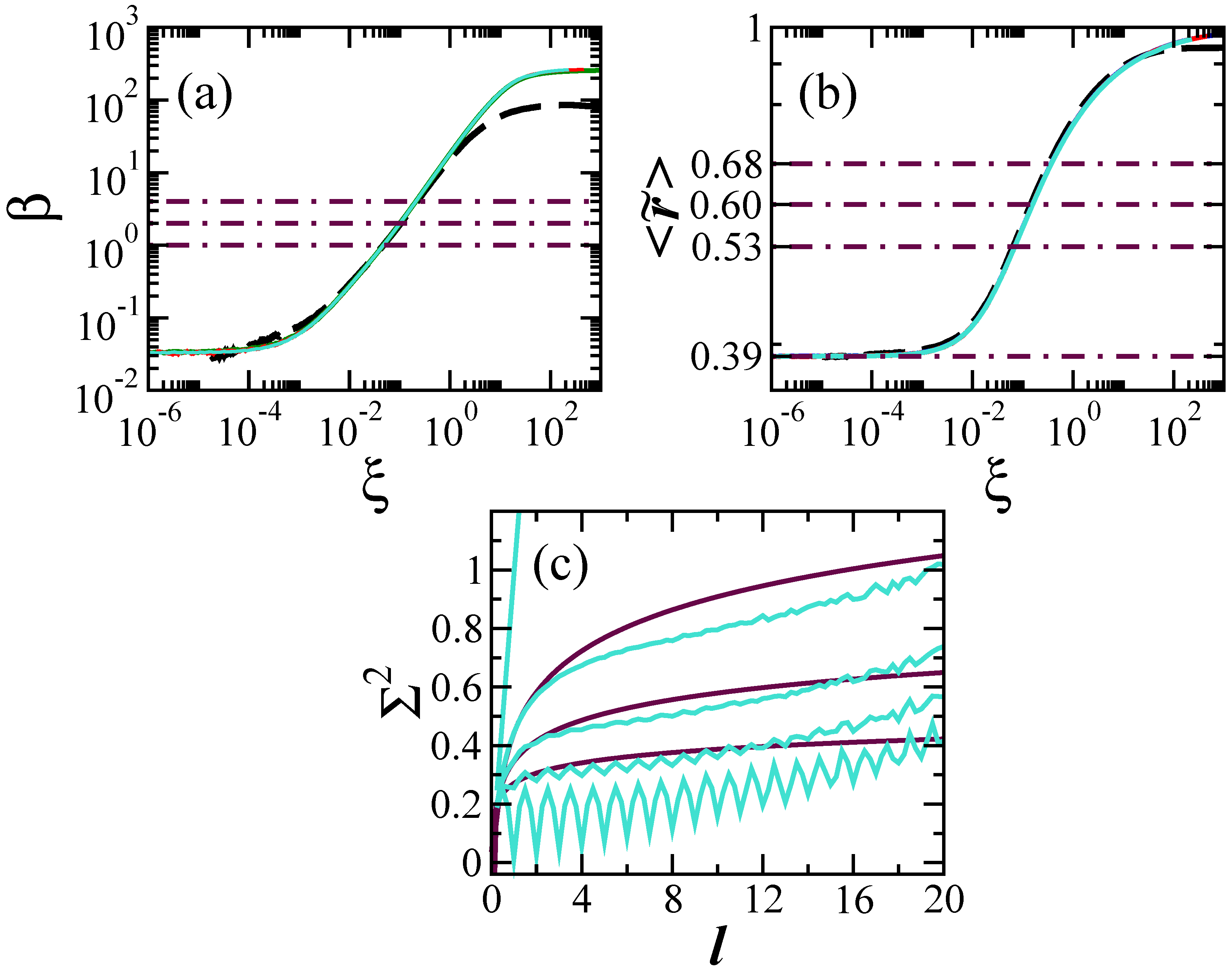
For the finite one-particle 1D Aubry-André model, the distribution is Poissonian when h is large. As the disorder strength decreases towards zero, where the eigenvalues become nearly equidistant, passes through all forms mentioned above, from Poisson to GOE-like, from GOE-like to GUE-like, from GUE-like to GSE-like, and finally from GSE-like to the picket-fence case, with all the intermediate distributions between each specific case. This is shown in Figure 1a,b.
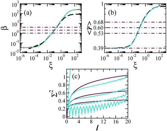
Figure 1.
Level repulsion parameter (a) and average ratio of spacings between consecutive levels as a function of , and level number variance (c). (a,b) Four system sizes are considered, and 4000. The four curves overlap, except for the smallest one in panel (a). The horizontal dot-dashed lines indicate the values for the Gaussian orthogonal ensemble (GOE), Gaussian unitary ensemble (GUE), and Gaussian symplectic ensemble (GSE) from top to bottom. (c) Numerical results for (light color) and analytical curves for GOE, GUE, and GSE (dark color). The numerical curves from top to bottom have values of that, according to , lead to the Poissonian distribution, GOE shape, GUE shape, GSE shape, and the picket-fence spectrum for . In all panels: averages over random realizations.
In Figure 1a, we show the values of obtained with the expression [55],
where A and B come from the normalization conditions
The values of are shown as a function of the ratio . This scaling factor collapses the curves for different system sizes on a single curve. In Figure 1b, we depict as a function of . While both and capture the crossovers from the Poissonian distribution up to the picket-fence spectrum as increases, it is evident that there is not an exact one-to-one correspondence between the two, but a more systematic comparison of the two quantities together with a careful unfolding procedure is worth doing. In this case, various different models should be taken into account, including true chaotic models.
It is important to emphasize that the different level spacing distributions obtained with the model are not linked with the symmetries of the Hamiltonian. The Hamiltonian matrix used here is real and symmetric for any value of . The different forms of the distributions are rather a consequence of the changes in the level of correlations as one goes from uncorrelated eigenvalues for large disorder to nearly equidistant levels for the clean chain.
There are other theoretical studies where level statistics as in RMT were generated [56,57,58]. Those approaches are different from the one taken in the present work, where we do not build the matrix elements with the purpose of generating specific level statistics; instead, they emerge due to finite size effects.
2.1.2. Long-Range Correlations
The analysis of long-range correlations can be done with the level number variance; that is, the variance of the unfolded levels in the interval ℓ. For uncorrelated eigenvalues, grows linearly with ℓ. In the case of full random matrices, we have for the GOE [11],
for the GUE,
and for the GSE,
where is Euler’s constant. For equidistant levels, as in the case of the harmonic oscillator, .
The plot of in Figure 1c makes it clear that the level of rigidity of the spectrum of the finite one-particle 1D Aubry-André model is not equivalent to that for full random matrices. There is agreement for very small ℓ, but then, for an interval of values of ℓ, the correlations are stronger in the Aubry-André model, until this behavior switches at large values of ℓ (compare the light and dark curves). As for the picket-fence spectrum for the clean chain (bottom light curve), we attribute the oscillations and the latter growth with ℓ to imperfections in the unfolding procedure and in the calculation of the level number variance, and to the fact that the eigenvalues are not exactly equidistant.
3. Evolution of the Number Operator
Let us prepare the system in a state , where the particle is either on the first site of the chain, , or on the middle one, . We then evolve it under H (1), . The quantity used in the analysis of the dynamics is the number operator,
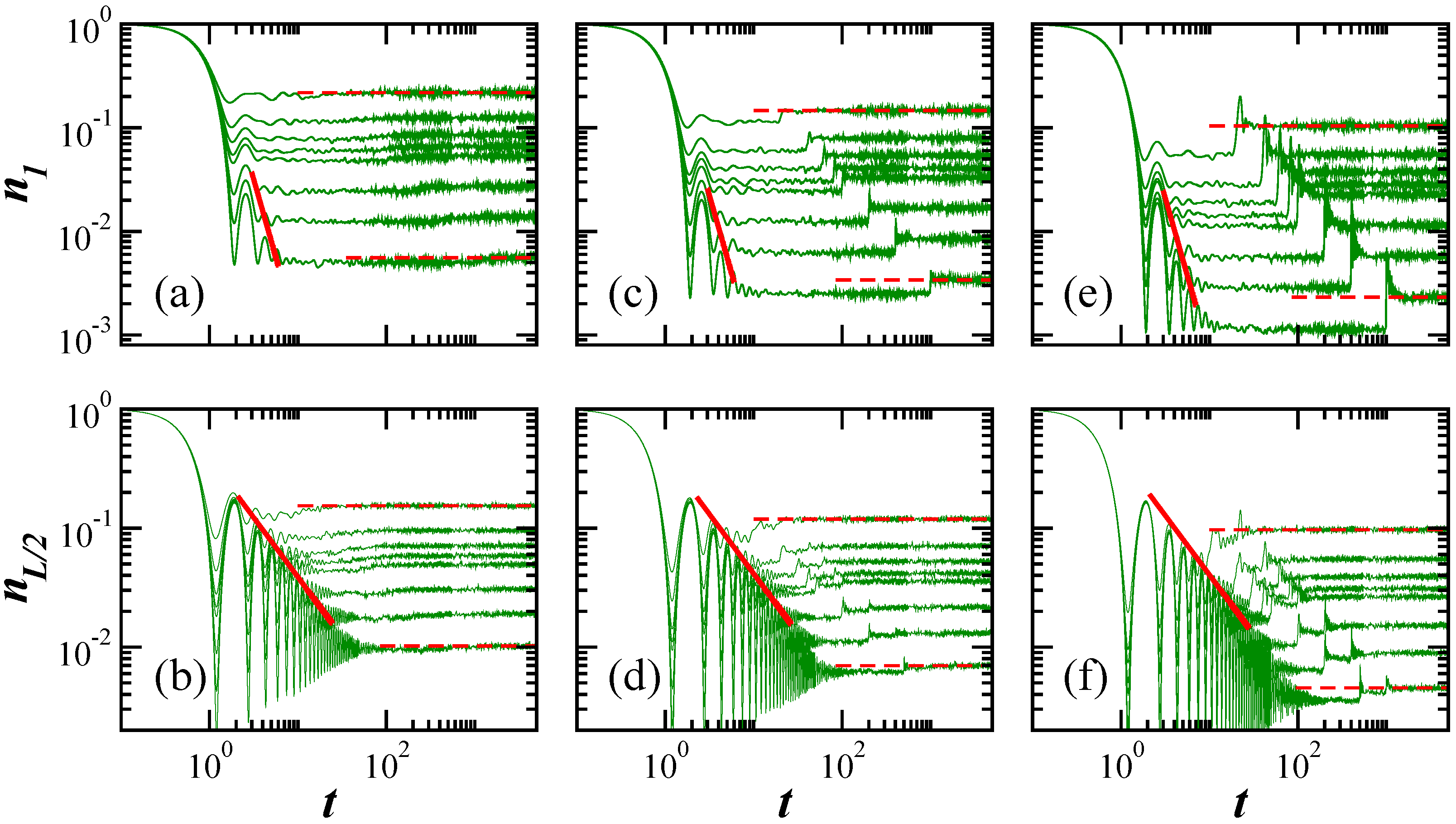
The results for and are shown in Figure 2 on the top [(a), (c), (e)] and bottom (b), (d), (f)] panels, respectively. In Figure 2a,b, the value of leads to the GOE-like level spacing distribution; in Figure 2c,d the distribution is GUE-like, and in Figure 2e,f is GSE-like.
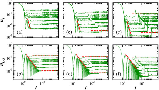
Figure 2.
Evolution of the number operator for a particle initially placed on Site 1 (a,c,e) and for one initially placed on Site (b,d,f) respectively, for spectra with GOE- (a,b), GUE- (c,d), and GSE-like (e,f) level spacing distributions. On each panel, the size L of the chain increases from top to bottom, . The red solid lines represent the power-law decays: for (a,c,e) and for (b,d,f). The horizontal dashed lines mark the saturation values for the smallest and largest L’s. In all panels: averages over random realizations.
The main result of Figure 2 is the fact that for experimental sizes (few dozens of sites), the correlation hole emerges at times () and values of the number operator () that are experimentally reachable. The correlation hole is the dip below the saturation point of the dynamics. In all panels of Figure 2, the saturation of the dynamics is marked with a red horizontal dashed line for the smallest and the largest system sizes. The correlation hole corresponds to the values of the numerical curves that are below this dashed line. The difference between saturation and minimum of the hole is most evident for the GSE-like spectrum in Figure 2e.
One can write the number operator in terms of the energy eigenstates and eigenvalues as
where is the lower bound of the spectrum and is the upper bound. In the equation above, the sum in parenthesis,
is the energy distribution of the initial state, often known as local density of states (LDOS) or strength function [59,60,61,62]. The number operator in Equation (10) is the square of the Fourier transform of the LDOS. We denote the variance of the LDOS by
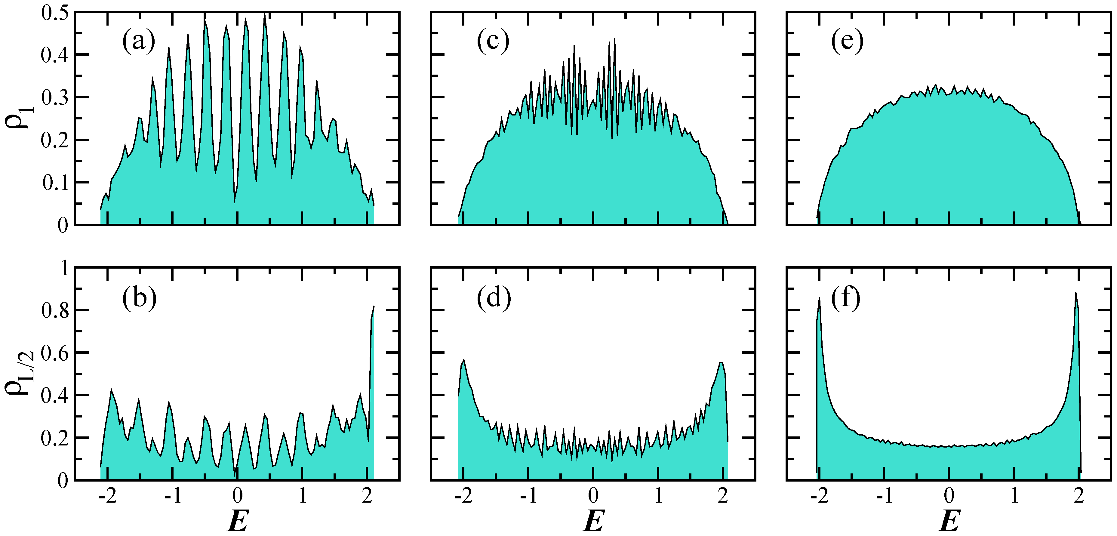
The envelope of the LDOS for the Hamiltonian with GOE-, GUE-, and GSE-like level spacing distributions is analogous to the shape obtained for the clean model [33]. It is a semicircle when and it has a U-shape when , as shown in Figure 3 for the GSE-like spectrum and three system sizes increasing from left to right, . For small sizes, such as , one sees approximately peaks in the middle of the LDOS. As L increases, the curves become smoother.
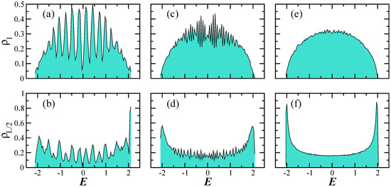
Figure 3.
Energy distribution of the initial state (LDOS) for a particle initially on Site 1 (a,c,e) and on Site (b,d,f) for spectra with GSE-like level spacing distribution. The sizes of the chain increase from left to right: (a,b); (c,d), (e,f). Average over random realizations.
The Fourier transform of the semicircle gives
and is the Bessel function of the first kind. For the U-shaped LDOS, we get
The equations above imply that the initial decay of is slower than for , which is noticeable by comparing the top and bottom panels of Figure 2 for . This is expected, since the particle on Site 1 can only hop to Site 2, while Site has two neighbors.
For , the picture changes and the dynamics become faster for than for . The quadratic decay is succeeded by a power-law decay that envelops the oscillations of the Bessel functions. This non-algebraic decay is caused by the bounds in the spectrum [63,64]. The exponent is for [65] and for [66].
The power-law decay is followed by a plateau that is below the saturation value,
of the number operator. This saturation point is marked with dashed horizontal lines in Figure 2. The plateau below this point corresponds to the correlation hole. It is related to the level number variance [11,37], which explains why it gets deeper as we move from the GOE- to the GUE- and to the GSE-like spectrum (compare Figure 1c and Figure 2). The hole does not develop in integrable models where the level spacing distribution is Poissonian and the eigenvalues are uncorrelated. But it does emerge in integrable models with a picket-fence spectrum.
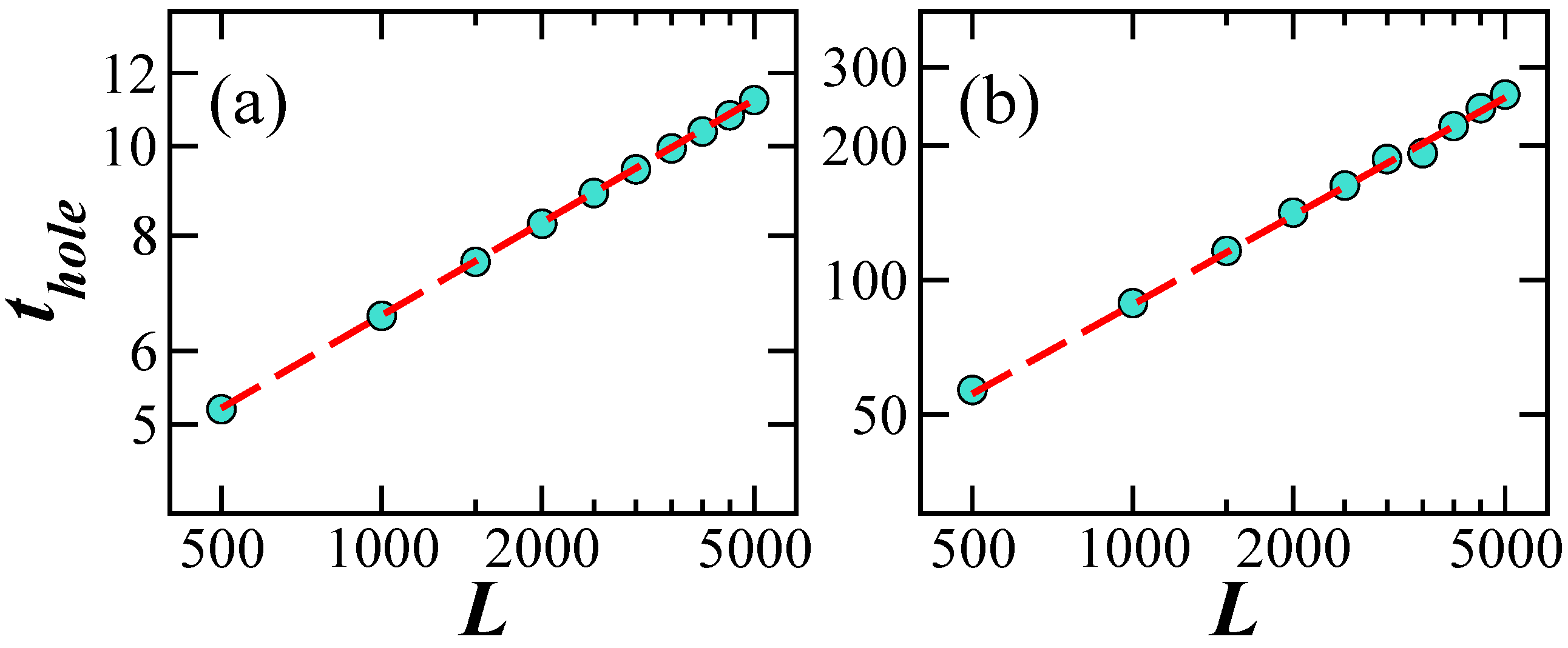
By checking where the curve of the power-law decay first crosses the plateau below , we estimate numerically, the time for the minimum of the correlation hole. As shown in Figure 4, we find that for and for . The first estimate can be derived from the fact that the power-law decay is and the minimum value of at the plateau is . The estimate for the for comes from the power-law decay and the minimum value of at the plateau, which is . Both times should be reachable by current experiments with cold atoms realized with few dozens of sites.
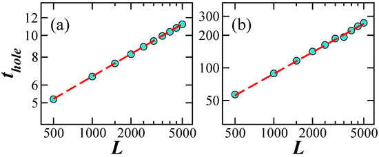
Figure 4.
Log–log plots for the time to reach the correlation hole for a particle initially placed on Site 1 (a) and a particle initially placed on Site (b) versus the system size for spectra with GSE-like level spacing distributions. (a) and (b) . Average over random realizations.
The correlation hole holds up to the revival of the dynamics, which first happens at for and at for , as seen in Figure 2. The revival is followed by another decay and a possible correlation hole, but at higher values. This behavior is better seen for the GSE-like spectrum in Figure 2f, where the correlation is deep. The revival repeats itself at for and at for with an yet larger value of the correlation hole. This second revival is better seen for larger L’s. We may expect subsequent revivals to become visible to even larger system sizes, although they should eventually become indistinguishable of the temporal fluctuations at the saturation point.
4. Conclusions
This work shows that the effects of level repulsion can be directly observed by studying the evolution of the number operator in the finite one-particle 1D Aubry-André model. Level repulsion is manifested in the form of the so-called correlation hole. The number operator, the Aubry-André model, the system sizes, and timescales studied here are accessible to experiments with cold atoms.
Author Contributions
All authors contributed equally. All authors have read and agreed to the published version of the manuscript.
Funding
E.J.T.-H. acknowledges funding from VIEP-BUAP (grant numbers MEBJ-EXC19-G and LUAG-EXC19-G). L.F.S. was supported by the NSF, grant number DMR-1936006.
Acknowledgments
E.J.T.H. is grateful to LNS-BUAP for allowing use of their supercomputing facility.
Conflicts of Interest
The authors declare no conflict of interest.
References
- Kitaev, A. Kitp Talk. 2015. Available online: http://online.kitp.ucsb.edu/online/entangled15/kitaev/ (accessed on 15 June 2016).
- Maldacena, J.; Stanford, D. Remarks on the Sachdev-Ye-Kitaev model. Phys. Rev. D 2016, 94, 106002. [Google Scholar] [CrossRef]
- Maldacena, J.; Shenker, S.H.; Stanford, D. A bound on chaos. J. High Energy Phys. 2016, 2016, 106. [Google Scholar] [CrossRef]
- Daniel, A. Roberts and Douglas Stanford. Diagnosing chaos using four-point functions in two-dimensional conformal field theory. Phys. Rev. Lett. 2015, 115, 131603. [Google Scholar]
- Fan, R.; Zhang, P.; Shen, H.; Zhai, H. Out-of-time-order correlation for many-body localization. Sci. Bull. 2017, 62, 707–711. [Google Scholar] [CrossRef]
- Luitz, D.J.; Lev, Y.B. Information propagation in isolated quantum systems. Phys. Rev. B 2017, 96, 020406. [Google Scholar] [CrossRef]
- Borgonovi, F.; Izrailev, F.M.; Santos, L.F. Timescales in the quench dynamics of many-body quantum systems: Participation ratio versus out-of-time ordered correlator. Phys. Rev. E 2019, 99, 052143. [Google Scholar] [CrossRef] [PubMed]
- Yan, H.; Wang, J.; Wang, W. Similar early growth of out-of-time-ordered correlators in quantum chaotic and integrable ising chains. arXiv 2019, arXiv:1906.11775. [Google Scholar] [CrossRef]
- García-Mata, I.; Saraceno, M.; Jalabert, R.A.; Roncaglia, A.J.; Wisniacki, D.A. Chaos signatures in the short and long time behavior of the out-of-time ordered correlator. arXiv 2018, arXiv:1806.04281. [Google Scholar]
- Bohigas, O.; Giannoni, M.; Schmit, C. Spectral fluctuations of classically chaotic quantum systems. Lect. Notes Phys. 1986, 263, 18. [Google Scholar]
- Guhr, T.; Mueller-Gröeling, A.; Weidenmüller, H.A. Random matrix theories in quantum physics: Common concepts. Phys. Rep. 1998, 299, 189. [Google Scholar] [CrossRef]
- Haake, F. Quantum Signatures of Chaos; Springe: Berlin, Gremany, 1991. [Google Scholar]
- Stöckmann, H.-J. Quantum Chaos: An Introduction; Cambridge University Press: Cambridge, UK, 2006. [Google Scholar]
- Rozenbaum, E.B.; Ganeshan, S.; Galitski, V. Lyapunov exponent and out-of-time-ordered correlator’s growth rate in a chaotic system. Phys. Rev. Lett. 2017, 118, 086801. [Google Scholar] [CrossRef] [PubMed]
- Jalabert, R.A.; García-Mata, I.; Wisniacki, D.A. Semiclassical theory of out-of-time-order correlators for low-dimensional classically chaotic systems. Phys. Rev. E 2018, 98, 062218. [Google Scholar] [CrossRef]
- Rozenbaum, E.B.; Ganeshan, S.; Galitski, V. Universal level statistics of the out-of-time-ordered operator. arXiv 2018, arXiv:1801.10591. [Google Scholar] [CrossRef]
- Chávez-Carlos, J.; López-del Carpio, B.; Bastarrachea-Magnani, M.A.; Stránský, P.; Lerma-Hernández, S.; Santos, L.F.; Hirsch, J.G. Quantum and classical Lyapunov exponents in atom-field interaction systems. Phys. Rev. Lett. 2019, 122, 024101. [Google Scholar] [CrossRef]
- Lewis-Swan, R.J.; Safavi-Naini, A.; Bollinger, J.J.; Rey, A.M. Unifying scrambling, thermalization and entanglement through measurement of fidelity out-of-time-order correlators in the Dicke model. Nat. Commun. 2019, 10, 1581. [Google Scholar] [CrossRef]
- Pappalardi, S.; Russomanno, A.; Zunkovic, B.; Iemini, F.; Silva, A.; Rosario, F. Scrambling and entanglement spreading in long-range spin chains. Phys. Rev. B 2018, 98, 134303. [Google Scholar] [CrossRef]
- Hummel, Q.; Geiger, B.; Urbina, J.D.; Richter, K. Reversible quantum information spreading in many-body systems near criticality. Phys. Rev. Lett. 2019, 123, 160401. [Google Scholar] [CrossRef]
- Pilatowsky-Cameo, S.; Chávez-Carlos, J.; Bastarrachea-Magnani, M.A.; Stránský, P.; Lerma-Hernández, S.; Santos, L.F.; Hirsch, J.G. Positive quantum Lyapunov exponents in classically regular systems. arXiv 2019, arXiv:1909.02578. [Google Scholar]
- Schreiber, M.; Hodgman, S.S.; Bordia, P.; Lüschen, H.P.; Fischer, M.H.; Vosk, R.; Altman, E.; Schneider, U.; Bloch, I. Observation of many-body localization of interacting fermions in a quasirandom optical lattice. Science 2015, 349, 842–845. [Google Scholar] [CrossRef]
- Harper, P.G. Single band motion of conduction electrons in a uniform magnetic field. Proc. Phys. Soc. A 1955, 68, 874–878. [Google Scholar] [CrossRef]
- Aubry, S.; André, G. Analyticity breaking and Anderson localization in incommensurate lattices. Ann. Isr. Phys. Soc. 1980, 3, 18. [Google Scholar]
- Sokoloff, J.B. Unusual band structure, wave functions and electrical conductance in crystals with incommensurate periodic potentials. Phys. Rep. 1985, 126, 189–244. [Google Scholar] [CrossRef]
- Domínguez-Castro, G.A.; Paredes, R. The Aubry-André model as the hobbyhorse for understanding localization phenomenon. arXiv 2018, arXiv:1812.06201. [Google Scholar] [CrossRef]
- Roy, N.; Sharma, A. Study of counterintuitive transport properties in the aubry-andré-harper model via entanglement entropy and persistent current. Phys. Rev. B 2019, 100, 195143. [Google Scholar] [CrossRef]
- Anderson, P.W. Absence of diffusion in certain random lattices. Phys. Rev. 1958, 109, 1492. [Google Scholar] [CrossRef]
- Lee, P.A.; Ramakrishnan, T.V. Disordered electronic systems. Rev. Mod. Phys. 1985, 57, 287–337. [Google Scholar] [CrossRef]
- Kramer, B.; MacKinnon, A. Localization: Theory and experiment. Rep. Prog. Phys. 1993, 56, 1469. [Google Scholar] [CrossRef]
- Lagendijk, A.; Van Tiggelen, B.; Wiersma, D.S. Fifty years of Anderson localization. Phys. Today 2009, 62, 24. [Google Scholar] [CrossRef]
- Sorathia, S.; Izrailev, F.M.; Zelevinsky, V.G.; Celardo, G.L. From closed to open one-dimensional Anderson model: Transport versus spectral statistics. Phys. Rev. E 2012, 86, 011142. [Google Scholar] [CrossRef]
- Torres-Herrera, E.J.; Méndez-Bermúdez, J.A.; Santos, L.F. Level repulsion and dynamics in the finite one-dimensional Anderson model. Phys. Rev. E 2019, 100, 022142. [Google Scholar] [CrossRef]
- Leviandier, L.; Lombardi, M.; Jost, R.; Pique, J.P. Fourier transform: A tool to measure statistical level properties in very complex spectra. Phys. Rev. Lett. 1986, 56, 2449–2452. [Google Scholar] [CrossRef]
- Guhr, T.; Weidenmüller, H.A. Correlations in anticrossing spectra and scattering theory. analytical aspects. Chem. Phys. 1990, 146, 21–38. [Google Scholar] [CrossRef]
- Wilkie, J.; Brumer, P. Time-dependent manifestations of quantum chaos. Phys. Rev. Lett. 1991, 67, 1185–1188. [Google Scholar] [CrossRef] [PubMed]
- Alhassid, Y.; Levine, R.D. Spectral autocorrelation function in the statistical theory of energy levels. Phys. Rev. A 1992, 46, 4650–4653. [Google Scholar] [CrossRef]
- Gorin, T.; Seligman, T.H. Signatures of the correlation hole in total and partial cross sections. Phys. Rev. E 2002, 65, 026214. [Google Scholar] [CrossRef] [PubMed]
- Torres-Herrera, E.J.; Santos, L.F. Extended nonergodic states in disordered many-body quantum systems. Ann. Phys. (Berlin) 2017, 529, 1600284. [Google Scholar] [CrossRef]
- Torres-Herrera, E.J.; Santos, L.F. Dynamical manifestations of quantum chaos: Correlation hole and bulge. Philos. Trans. Royal Soc. A 2017, 375, 20160434. [Google Scholar] [CrossRef]
- Torres-Herrera, E.J.; García-García, A.M.; Santos, L.F. Generic dynamical features of quenched interacting quantum systems: Survival probability, density imbalance, and out-of-time-ordered correlator. Phys. Rev. B 2018, 97, 060303. [Google Scholar] [CrossRef]
- Cotler, J.S.; Gur-Ari, G.; Hanada, M.; Polchinski, J.; Saad, P.; Shenker, S.H.; Stanford, D.; Streicher, A.; Tezuka, M. Black holes and random matrices. J. High Energy Phys. 2017, 2017, 118. [Google Scholar] [CrossRef]
- Numasawa, T. Late time quantum chaos of pure states in random matrices and in the sachdev-ye-kitaev model. Phys. Rev. D 2019, 100, 126017. [Google Scholar] [CrossRef]
- Schiulaz, M.; Torres-Herrera, E.J.; Santos, L.F. Thouless and relaxation time scales in many-body quantum systems. Phys. Rev. B 2019, 99, 174313. [Google Scholar] [CrossRef]
- Lerma-Hernández, S.; Villaseñor, D.; Bastarrachea-Magnani, M.A.; Torres-Herrera, E.J.; Santos, L.F.; Hirsch, J.G. Dynamical signatures of quantum chaos and relaxation time scales in a spin-boson system. Phys. Rev. E 2019, 100, 012218. [Google Scholar] [CrossRef] [PubMed]
- Singh, K.; Fujiwara, C.J.; Geiger, Z.A.; Simmons, E.Q.; Lipatov, M.; Cao, A.; Dotti, P.; Rajagopal, S.V.; Senaratne, R.; Shimasaki, T.; et al. Quantifying and controlling prethermal nonergodicity in interacting Floquet matter. arXiv 2018, arXiv:1809.05554. [Google Scholar] [CrossRef]
- Griniasty, M.; Fishman, S. Localization by pseudorandom potentials in one dimension. Phys. Rev. Lett. 1988, 60, 1334–1337. [Google Scholar] [CrossRef] [PubMed]
- Mehta, M.L. Random Matrices; Academic Press: Boston, MA, USA, 1991. [Google Scholar]
- Oganesyan, V.; Huse, D.A. Localization of interacting fermions at high temperature. Phys. Rev. B 2007, 75, 155111. [Google Scholar] [CrossRef]
- Atas, Y.Y.; Bogomolny, E.; Giraud, O.; Roux, G. Distribution of the ratio of consecutive level spacings in random matrix ensembles. Phys. Rev. Lett. 2013, 110, 084101. [Google Scholar] [CrossRef]
- Gómez, J.M.G.; Molina, R.A.; Relaño, A.; Retamosa, J. Misleading signatures of quantum chaos. Phys. Rev. E 2002, 66, 036209. [Google Scholar] [CrossRef]
- Berry, M.V.; Tabor, M. Level clustering in the regular spectrum. Proc. R. Soc. Lond. A 1997, 356, 375–394. [Google Scholar] [CrossRef]
- Pandey, A.; Ramaswamy, R. Level spacings for harmonic-oscillator systems. Phys. Rev. A 1991, 43, 4237–4243. [Google Scholar] [CrossRef]
- Chirikov, B.V.; Shepelyansky, D.L. Shnirelman peak in level spacing statistics. Phys. Rev. Lett. 1995, 74, 518–521. [Google Scholar] [CrossRef]
- Izrailev, F.M. Simple models of quantum chaos: Spectrum and eigenfunctions. Phys. Rep. 1990, 196, 299–392. [Google Scholar] [CrossRef]
- Wu, H.; Sprung, D.W.L.; Feng, D.H.; Vallières, M. Modeling chaotic quantum systems by tridiagonal random matrices. Phys. Rev. E 1993, 47, 4063–4066. [Google Scholar] [CrossRef] [PubMed]
- Zhang, W.-M.; Feng, D.H. Quantum nonintegrability in finite systems. Phys. Rep. 1995, 252, 1–100. [Google Scholar] [CrossRef]
- Relaño, A.; Dukelsky, J.; Gómez, J.M.G.; Retamosa, J. Stringent numerical test of the poisson distribution for finite quantum integrable hamiltonians. Phys. Rev. E 2004, 70, 026208. [Google Scholar] [CrossRef] [PubMed]
- Flambaum, V.V.; Gribakina, A.A.; Gribakin, G.F.; Kozlov, M.G. Structure of compound states in the chaotic spectrum of the ce atom: Localization properties, matrix elements, and enhancement of weak perturbations. Phys. Rev. A 1994, 50, 267–296. [Google Scholar] [CrossRef]
- Angom, D.; Ghosh, S.; Kota, V.K.B. Strength functions, entropies, and duality in weakly to strongly interacting fermionic systems. Phys. Rev. E 2004, 70, 016209. [Google Scholar] [CrossRef]
- Izrailev, F.M.; Castañeda-Mendoza, A. Return probability: Exponential versus Gaussian decay. Phys. Lett. A 2006, 350, 355–362. [Google Scholar] [CrossRef]
- Torres-Herrera, E.J.; Santos, L.F. Quench dynamics of isolated many-body quantum systems. Phys. Rev. A 2014, 89, 043620. [Google Scholar] [CrossRef]
- Távora, M.; Torres-Herrera, E.J.; Santos, L.F. Inevitable power-law behavior of isolated many-body quantum systems and how it anticipates thermalization. Phys. Rev. A 2016, 94, 041603. [Google Scholar] [CrossRef]
- Távora, M.; Torres-Herrera, E.J.; Santos, L.F. Power-law decay exponents: A dynamical criterion for predicting thermalization. Phys. Rev. A 2017, 95, 013604. [Google Scholar] [CrossRef]
- Torres-Herrera, E.J.; Kollmar, D.; Santos, L.F. Relaxation and thermalization of isolated many-body quantum systems. Phys. Scr. T 2015, 165, 014018. [Google Scholar] [CrossRef]
- Santos, L.F.; Távora, M.; Pérez-Bernal, F. Excited-state quantum phase transitions in many-body systems with infinite-range interaction: Localization, dynamics, and bifurcation. Phys. Rev. A 2016, 94, 012113. [Google Scholar] [CrossRef]
© 2020 by the authors. Licensee MDPI, Basel, Switzerland. This article is an open access article distributed under the terms and conditions of the Creative Commons Attribution (CC BY) license (http://creativecommons.org/licenses/by/4.0/).

