Article

Observing Dynamical Systems Using Magneto-Controlled Diffraction

1
Soft Matter Lab, School of Arts, Sciences and Humanities, University of São Paulo, São Paulo 03828-000, Brazil
2
Ferrocell USA, 739 Route 259, Ligonier, PA 15658, USA
3
Technical Space Science Center, 235, Martindale Drive, Morehead State University, Morehead, KY 40531, USA
*
Author to whom correspondence should be addressed.
Condens. Matter 2019, 4(2), 35; https://doi.org/10.3390/condmat4020035
Submission received: 26 February 2019 / Revised: 25 March 2019 / Accepted: 26 March 2019 / Published: 28 March 2019

Abstract

:
Observing the light passing through a thin layer of ferrofluid, we can see the occurrence of interesting effects, both in the formation patterns within the ferrofluid layer and in the dispersion of light outside that layer. This leads us to ask what the explanations associated with these effects are. In this paper, we analyze and explain the occurrence of these luminous patterns using a Ferrolens, commercially known as a Ferrocell. We present details of our experimental apparatus, followed by a discussion of some properties of light polarization and its relation to the formation of magnetic contours produced by a Ferrolens. In addition, we present the observation of a magnetochiral effect in this system. Next, we propose an application of this experiment in dynamical systems. The dynamical system is the direct observation of diffracted lines in Ferrolens, a special case of a Hele-Shaw cell containing a transparent ferrofluid subjected to various light sources.

1. Introduction

When the light passes through a thin layer of ferrofluid, we can observe directly with the naked eye the formation of interesting luminous patterns. A device created for observation of these patterns is the Ferrolens, invented by Timm A. Vanderelli, (a contributing author), as shown in Figure 1. We applied this device to study dynamical systems. Dynamical systems can be described in the abstract space known as phase space, which represents the evolution of the solutions of this system from quantities as a function of time. In such systems, we can explore the geometry of these solutions and the correlated changes, when some parameter controlling the dynamical system is varied. In this space, we can recognize a variety of points, called node, saddle, focus, vortex, and so on, formed by the set of solutions [1]. For example, the solutions of a pendulum with just two independent modes of oscillation can be represented in a surface of a torus anchored in two points, and the collection of solutions is called an “attractor.” The stability of different types of attractors is related to the distribution of singular points around them, as in the case of the mechanical stability, which is represented by the potential energy of some object disturbed by small displacements, with stable, unstable, and indifferent equilibrium, so that we can describe the motion of this object subjected to Newton’s law of mechanics. This work aims to present a similar task, by using light and magnetic fields, inspired by the observation of light patterns in the Ferrolens [2], a device based on a Hele-Shaw cell containing ferrofluid, which can control light, acting as a magnetic lens.
The potential applications for this kind of device is remarkable, for example the observation of light patterns in ferrofluids motivated some authors: to compare them with some atmospheric optics phenomena [2]; or to understand the cause behind the existence of light patterns [3], known as magnetic contours; or considering the ferrofluids as “smart nanofluid” [4], we can find some interesting studies of the optical properties controlled by an external magnetic field, such as the formation of ring structures of light in scattered patterns [5]; or in some exciting applications such as liquid robotics [6]. In addition to these cases, we have applications of nanoparticles in the medical field, because nanomaterials can offer a way to treat cancer without causing much damage to healthy tissue [7,8].
The paper is structured as follows: in Section 2, we present our experimental apparatus and some methods of analysis. In Section 3.1, we discuss some aspects of light polarization and the formation of magnetic contours in the Ferrolens, along with the effects of the magnetic field in the Ferrolens and related light patterns. In Section 3.2, we report the observation of a magnetochiral effect. The application of the Ferrolens in dynamical systems is explored in Section 4. Finally, our concluding remarks are presented in Section 5.

2. Materials and Methods

We have developed a magneto-optical system which simulates the stability of fixed points and the trajectory of the orbits present in a dynamical system, using the Ferrolens shown in Figure 2.
The light pattern observed in the Ferrolens is based on the idea that when the ferrofluid is placed in the presence of a magnetic field, it can interact with light. The ferrofluid is a stable colloidal dispersion using light mineral oil (EFH1, Ferrotec), with the response time around 200 ms, typically containing 5% of magnetic solid, 10% of surfactant and 85% carrier. The nanoparticles are spheres of the order of 10 nm in diameter, and the carrier being the mineral oil. The nominal saturation magnetization value is 440 G. The magnetic volume fraction of EFH1 is 6.5, and more information about this ferrofluid can be found on the manufacturer’s website. The magneto-optic effect existing in this device results in the change of some optical parameters of the ferrofluid, such as the retardance [9], related to the refraction index, which is shown graphically in an approximated function of the retardance (R(B)) in Figure 3, for different values of ferrofluid concentrations, showing the general behavior of a sigmoidal curve as a function of the magnetic field. The Ferrolens is a Hele-Shaw cell containing the transparent ferrofluid and when fully dispersed it is only a few microns in thickness.
The magnetic field is obtained by placing some neodymium magnets facing the Ferrolens. The values of the magnetic field were obtained with a gaussmeter (Lakeshore, model 475 DSP), at room temperature of 24 °C, using a Hall sensor. Considering the plane of the Ferrolens in the horizontal position, the magnets were placed at the center of this plane, on the top of it. In this way, the magnets can create different magnetic field configurations, depending on their orientation. The detailed explanation of the positioning and measurements of the Hall sensor for the magnetic field of the compound magnets can be found in Figure 2 of Ref. [10]. The magnetic field of a cylinder magnet is a vector in the three-dimensional space, as shown in Figure 2. For the same magnet, we can observe two configurations, polar and dipolar, depending on the direction of the measurement. In Figure 4, we used a gaussmeter to obtain the magnetic field of each configuration, and the magnetic field intensities are enough to cause changes in the magneto-optical properties of the Ferrolens, such as Faraday rotation, dichroism, or birefringence. For example, in Figure 3 we present the plot of birefringence in the ferrofluid for different values of the magnetic field. This magnetic field passes through the plane delimited by the Ferrolens; thus, we just visualize the effects of the magnetic field projected in this plane, like the two patterns in Figure 2. In this way, the image obtained from the Ferrolens in Figure 2a is related to the magnetic field obtained with the gaussmeter of Figure 4b, and the light pattern of Figure 2b is associated with the magnetic field of Figure 4d. One way to see directly what is happening inside the Ferrolens is by obtaining the polarimetry of the Ferrolens, see References [2,3,4,10] for more detailed discussions about the light polarization effects of this device. We observed that the nanoparticles create a diffracting grating following the orientation of the magnetic field, forming a needle-like structure locally.
The light is diffracted by these nanoparticles following perpendicular scattered lines to the nanoparticles array. The light source is the origin of the light line, and each diffracted line is perpendicular to the ferrofluid needle-like structure. We used three different types of light source configurations to explore the effects of the light scattering in the Ferrolens that was subjected to an external magnetic field: laser green (collimated light with λ = 532 nm), high-intensity LED’s (non-collimated light with colors red with λ = 612 nm, green with λ = 519 nm, and blue with λ = 483 nm), and polarized light obtained with a white LED panel light, with crossed polarizers.
To register the patterns obtained with the Ferrolens, we used a digital camera placed at different positions from the Ferrolens. These images were reconstructed and analyzed using some routines written in C++, or commercial software, such as OriginLab for the case of pattern simulations of light polarization, computing matrices with 1000 × 1000 elements, Pic2Mag, and Maple programs.

3. Discussion

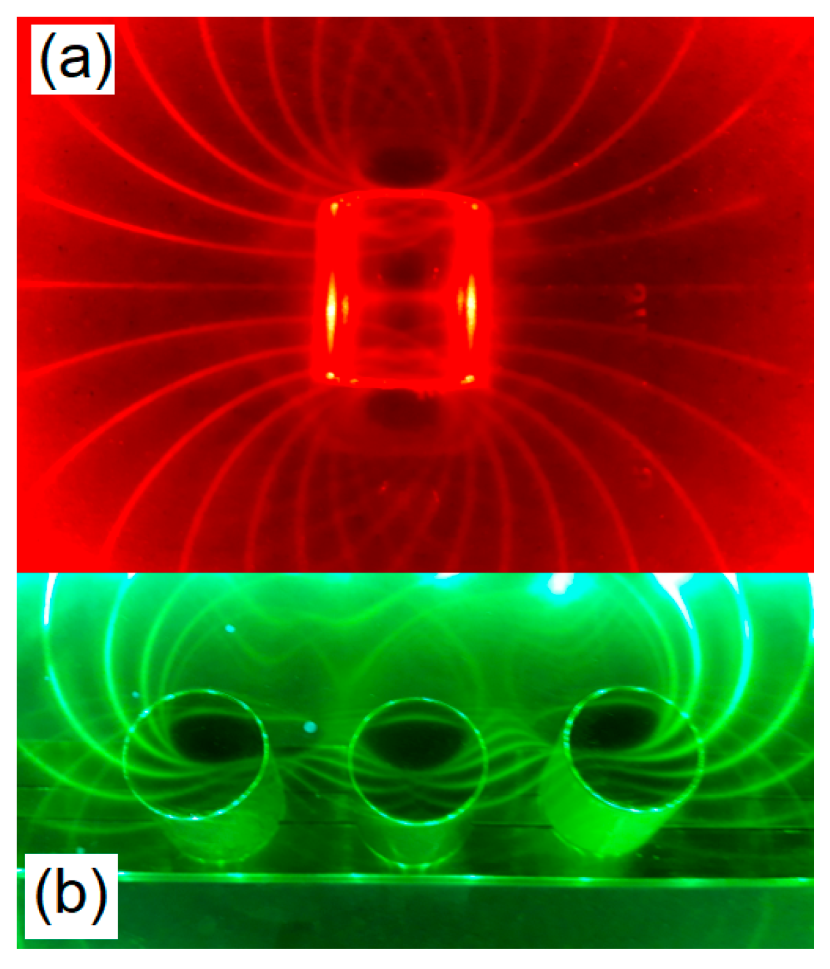
3.1. Light Polarization in Thin Film and Magnetic Contour Patterns

At very low fields (less than 1 G), the ferrofluids are isotropic, and light passes through the Ferrolens with almost no scattering because the magnetic nanoparticles behave as a single domain particle in a state of Brownian motion. Increasing the intensity of the magnetic field (around 500 G), approaching a magnet in the polar configuration 6 mm from the top of the Ferrolens, there are anisotropic effects, because aggregations of magnetic elongated particles along the field direction happen due to the strong interparticle interactions [10,11,12], like the macroscopic patterns of iron filings around a magnet. The light polarization patterns obtained from the experiment can be observed in Figure 5, Figure 6 and Figure 7 for some configurations of permanent magnets.
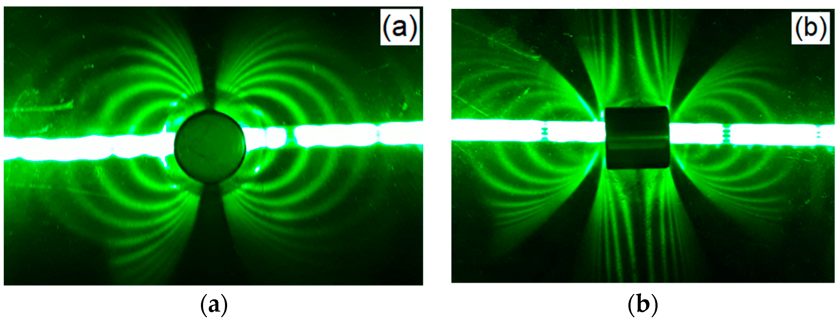
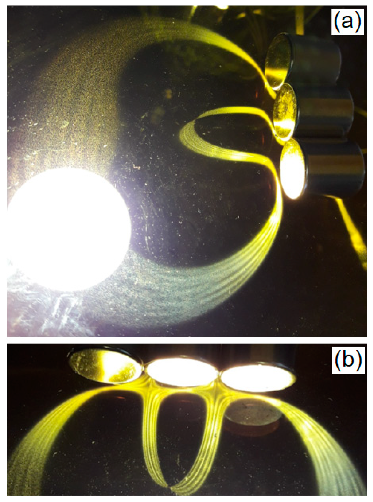
In Figure 5a, the Ferrolens is generating patterns for the case of polar configuration obtained from a magnet facing the Ferrolens, with the magnetic field represented previously in Figure 4b measuring the magnetic field in the plane X-Y. In Figure 6a there is the image of light polarization of the dipolar configuration of the magnetic field from Figure 4d. In Figure 7, we are presenting the case of the quadrupolar configuration, with the light pattern obtained without polarizers in Figure 7a with two magnets at the center of the figure. We can see the light polarization pattern in Figure 7b. In Figure 5b, Figure 6b and Figure 7c we are presenting the simulations of the light polarization of the Ferrolens in the presence of the respective magnetic field configurations. The main aspects of these simulations are discussed below.
By inspection, we have observed that some of these properties of light polarization are related to multiple diffraction problems and pattern formation. If U(x,y) and U′(x′,y′) represent the complex amplitudes of light over the surfaces of the Ferrolens, then by applying the Fresnel–Kirchhoff diffraction theory [13] we can write
U ( x , y ) = i k 4 π U ( x , y ) e i k r r ( 1 + c o s θ ) d x d y ,
in which r = [d2 + (x′-x)2 + (y′ − y)2]1/2 and cos θ = d/r. Without the ferrofluid, the two functions will become identical, but in the presence of the diffraction grating formed by the ferrofluid subjected to the magnetic field, there is a constant factor γ. In this case
γ U ( x , y ) = i k 4 π U ( x , y ) e i k r r ( 1 + c o s θ ) d x d y .
Although accurate solutions of this cavity problem are quite involved, it is possible to find a simple approximation by employing the same procedure as that of the Fraunhofer diffraction case, the function U(x,y) is its own Fourier transform. The simplest of such functions is the Gaussian, and the more general functions that are their own Fourier transforms are products of Hermite polynomials Hp and Hq:
U p q ( x , y ) = H p ( 2 x w ) H q ( 2 y w ) e ( x 2 + y 2 ) / w 2 .
In the presence of the external magnetic field configurations, we have observed the existence of some typical patterns. The observed pattern suggests a resemblance of the polarimetry of Ferrolens with the concept of spatial mode of Equation (3) and other hypergeometric polynomials empirically. We have approximated the intensity of light polarization I observed for magnetic field B [2,10] as
B ( x , y , z ) = B 0 H m ( x ) H n ( y ) e ( x 2 + y 2 ) / w 2 ( z ) e i φ ( z ) , I ( x , y , z ) = | B ( x , y , z ) | 2 ,
in which B0 is the maximal intensity of the magnetic field, Hm(x) and Hn(y) are the spatial derivatives of the magnetic field functions in the x-axis and y-axis respectively. I(x,y,z) is the light intensity directly observed from the Ferrolens with two crossed polarizers. These solutions are represented in the simulations of Figure 5b, Figure 6b and Figure 7c.
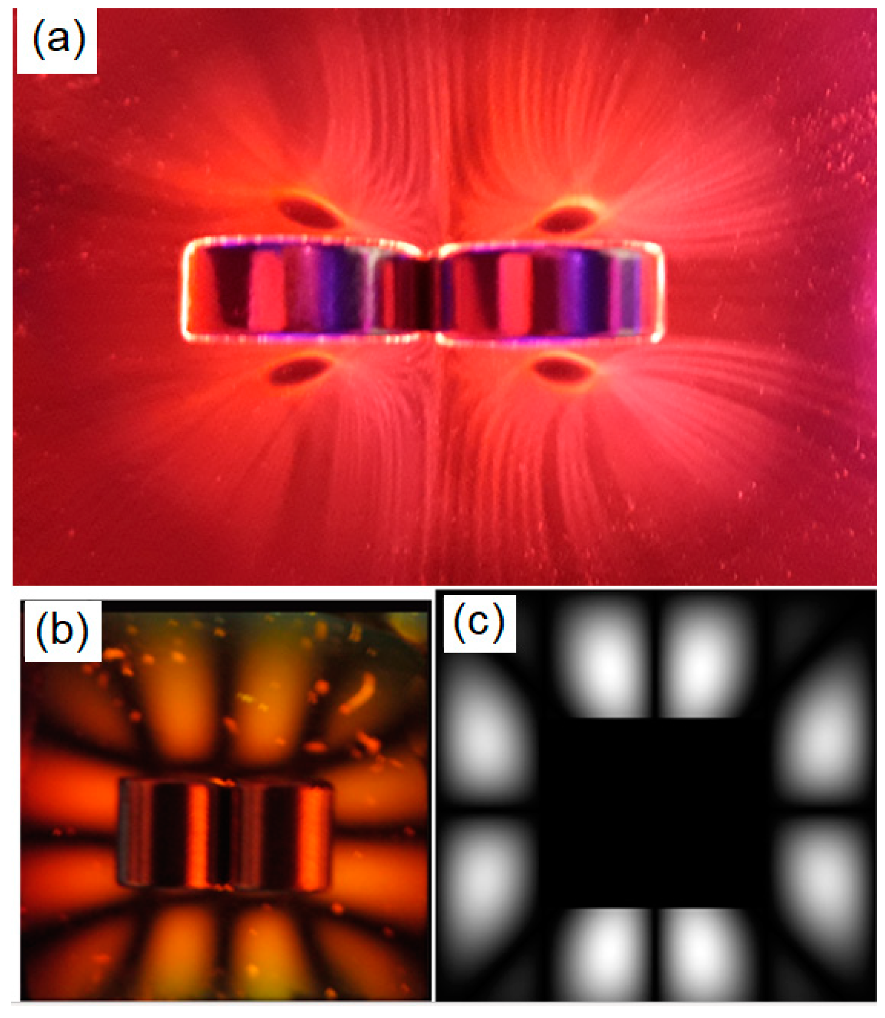
It is interesting to note the existence of the combination of diffraction and interference in this system. When a laser beam passes through this magnetic fluid placed in a magnetic field, it undergoes diffraction, producing characteristic patterns such as the jumping laser dogs [2]. The magneto-optical properties of this kind of combination of diffraction and interference was extensively studied by Philip et al. [4], summarized by the statement that the reason for the formation of curved light lines on the scattered pattern can be explained by considering scattering of light by cylinders and evaluating the scattered electromagnetic field from a cylindrical surface. The light diffracted by a spatial grating of magnetic chains is an integral sum of diffraction events from individual chains, and the observed patterns can be interpreted as a combination of diffraction and interference [10]. For magnetic fields intensities around 500 G, the formation of light patterns become sharper, and this behavior indicates the formation of smoothly surfaced columns. Some examples of these columns (nanoneedles) obtained from our experiment are given in Figure 8. For more details of this kind of agglomeration see Ref. [14].
The study of these agglomerates can be done in Ferrolens type devices to observe their evolution of biocompatible materials in the presence of magnetic fields, simulating the effects of these materials in conditions like those found in living tissues, where the flow is restricted due to the size of the vessels through which fluids flow, such as blood [7,8].
These concepts suggest a possible explanation for the magnetic contours observed in the Ferrolens based on the idea of magnetic potential. For the case of a magnetic scalar potential Vm, the magnets can be modeled as two magnetic charges Mc producing a magnetic dipole with [3]:
V m = μ M c 4 π [ 1 r n 1 r s ] ,
in which rn and rs is the position of poles north and south, respectively, and μ is the magnetic constant. The nanoparticles create a structure very similar to a diffracting grating from the influence of the orientation of a magnetic field. The light diffracted by the ferrofluids grating seemed to follow isopotential lines of this scalar field, having the light source as the origin of the light line, because each diffraction line is perpendicular to the scatterer. Starting with the case of the polar magnet configuration by considering (rs infinity), which reduces the magnetic potential to the case:
V m = μ M c 4 π 1 r n
This case gives us the representation of equipotential lines surrounding the pole of the magnet forming concentric circles. Since the magnitude of the magnetic potential decreases as 1/r with the distance from the source, lines representing equal jumps in potential are spaced closer together nearer to the north pole of the magnet and spaced farther apart away from this magnet pole. These concentric circles of the magnetic field form because of the symmetry of the magnetic pole, and hence the radial symmetry of the field suggested by the polar configuration of Equation (6).
The relationship between the diffracted lines and the magnetic potential is clear when considering a single dimension. In the one-dimensional case, r = x, so that Vm = constant/x. Hence the vector associated with light lines D and the magnetic scalar potential V is
D = d V d x î .
In other words, this relation means that the strength of the diffracted lines at any point in space is the rate of the change of the magnetic potential over space. If the magnetic potential changes significantly for a given distance, the diffracted line is strong, but if the magnetic potential changes only by a small amount at the same distance, the diffracted line is less intense. In addition to this, we have observed that these diffracted lines depend on the physical properties of the light source, such as polarization, states of collimation and intensity. Thus, we say that the diffracted lines mimic the gradient of the magnetic potential.
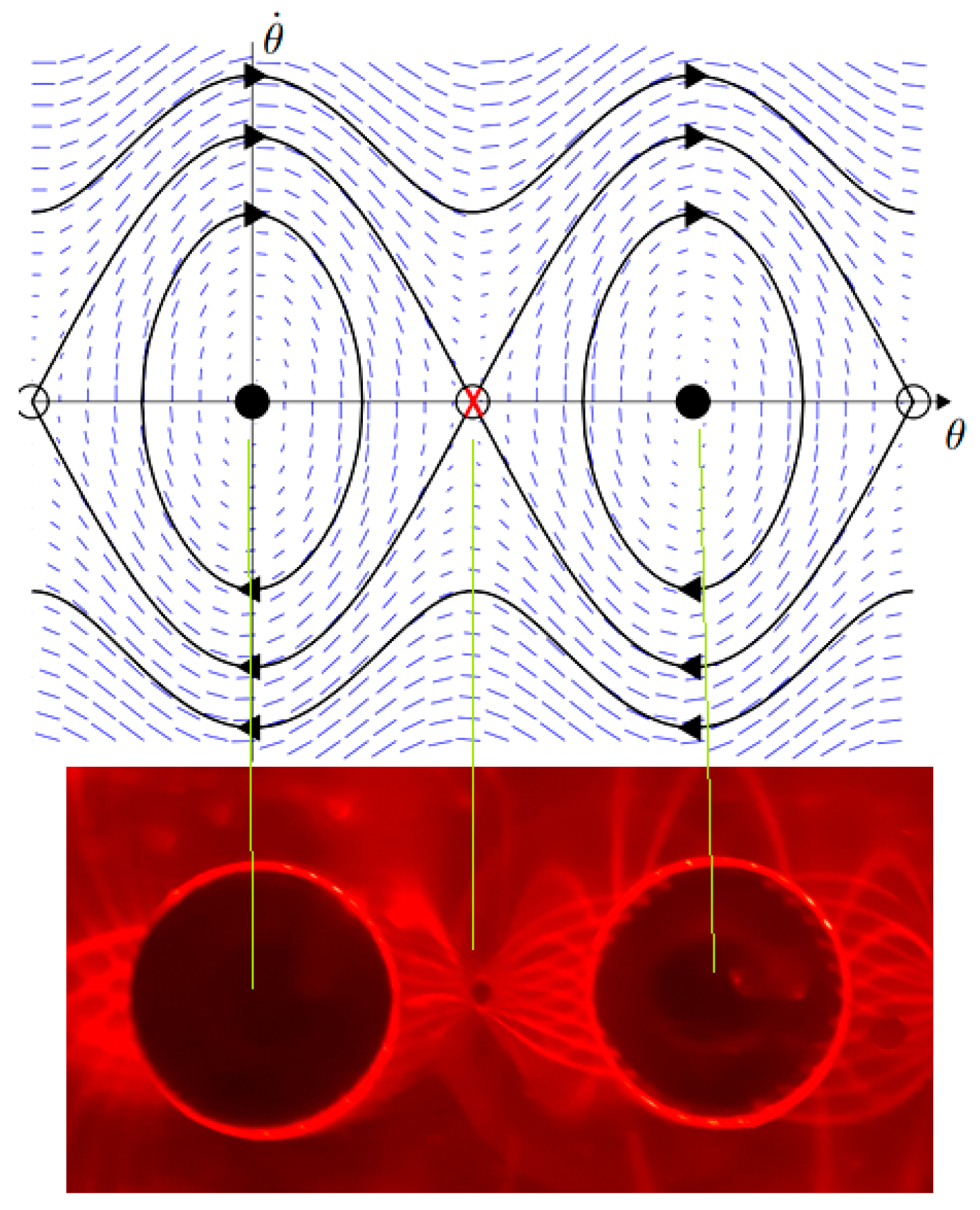
In this way, the magnetic contours are analogous to the orbits of dynamical systems, because these contours are associated to a vector field, and the trajectories of these orbits are obtained by the diffracted light, which consists of light patterns irradiated from the liquid film, and these light patterns can be related to some magneto-optical effects, depending on the relative position of the viewer and the light source. In Figure 9 we present the top view of two light patterns obtained using a straight line of LED’s, in the case of a polar configuration in Figure 9a and a dipolar configuration in Figure 9b, for the same straight line of LED’s. To exemplify the dependence of the position of the light source, in the case of the dipolar configuration in Figure 9b, we are presenting the pattern of Figure 10, the sequence of curved light lines from placing a straight line of LEDs far from the magnet.
The general pattern of the orbits does not depend on the wavelength of the light source, as it can be seen in Figure 11a,b for the same case of the dipolar configuration of Figure 9b, with light colors red and blue. In all these cases the light patterns do not cross each other, like the case of equipotential lines oriented by the magnetic field and the source of light as well.
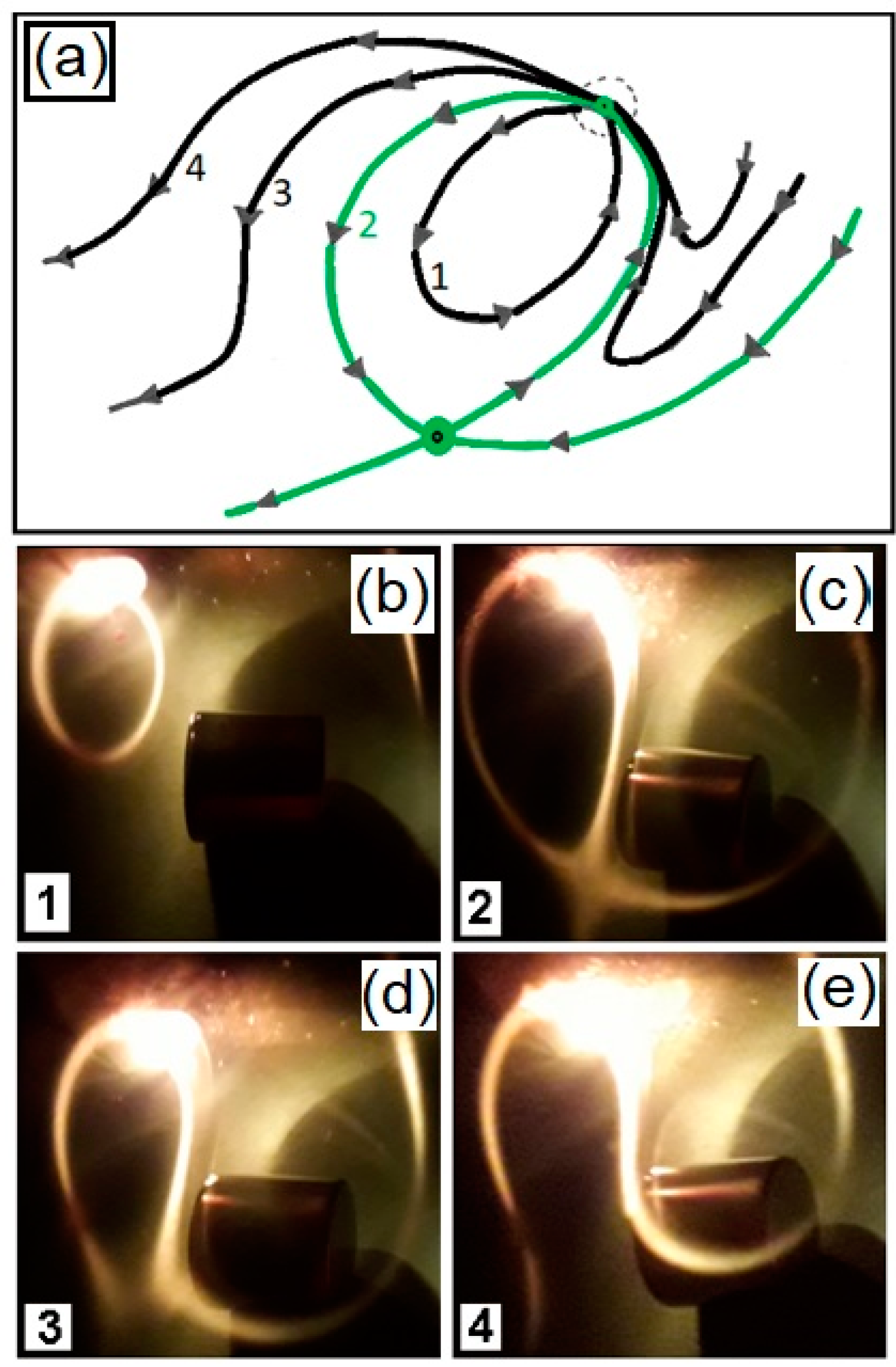
To reinforce the effect of collimated and uncollimated light source in the Ferrolens, we are presenting the case of light diffraction by transmission in Figure 12, which occurs when we used the laser beam (a coherent and collimated source of light) passing through the Ferrolens, while the formation of elliptical light patterns in the plane of the Ferrolens is caused by the light scattering of non-collimated light, forming patterns in a two-step process. This can be observed simultaneously in Figure 12, in which the first step is the diffraction of the green laser light through the Ferrolens in the presence of a magnetic field, projecting a curved line in the screen, with an intense light spot obtained due to the direct projection of the laser. The next step is obtained by the light spot of the laser hitting the screen, changing it to an uncollimated light source. The elliptical pattern is the result of this light spot affected by the magnetic field, or any kind of incoherent and not collimated light placed behind the Ferrolens, such as an LED, or an incandescent light. In Figure 13, we have a comparison between a simulation of the vector D and the light pattern obtained with Ferrolens, using various light sources of different colors. In this figure, we can observe that the phenomenon of line crossing is associated with different sources of light, as discussed previously.

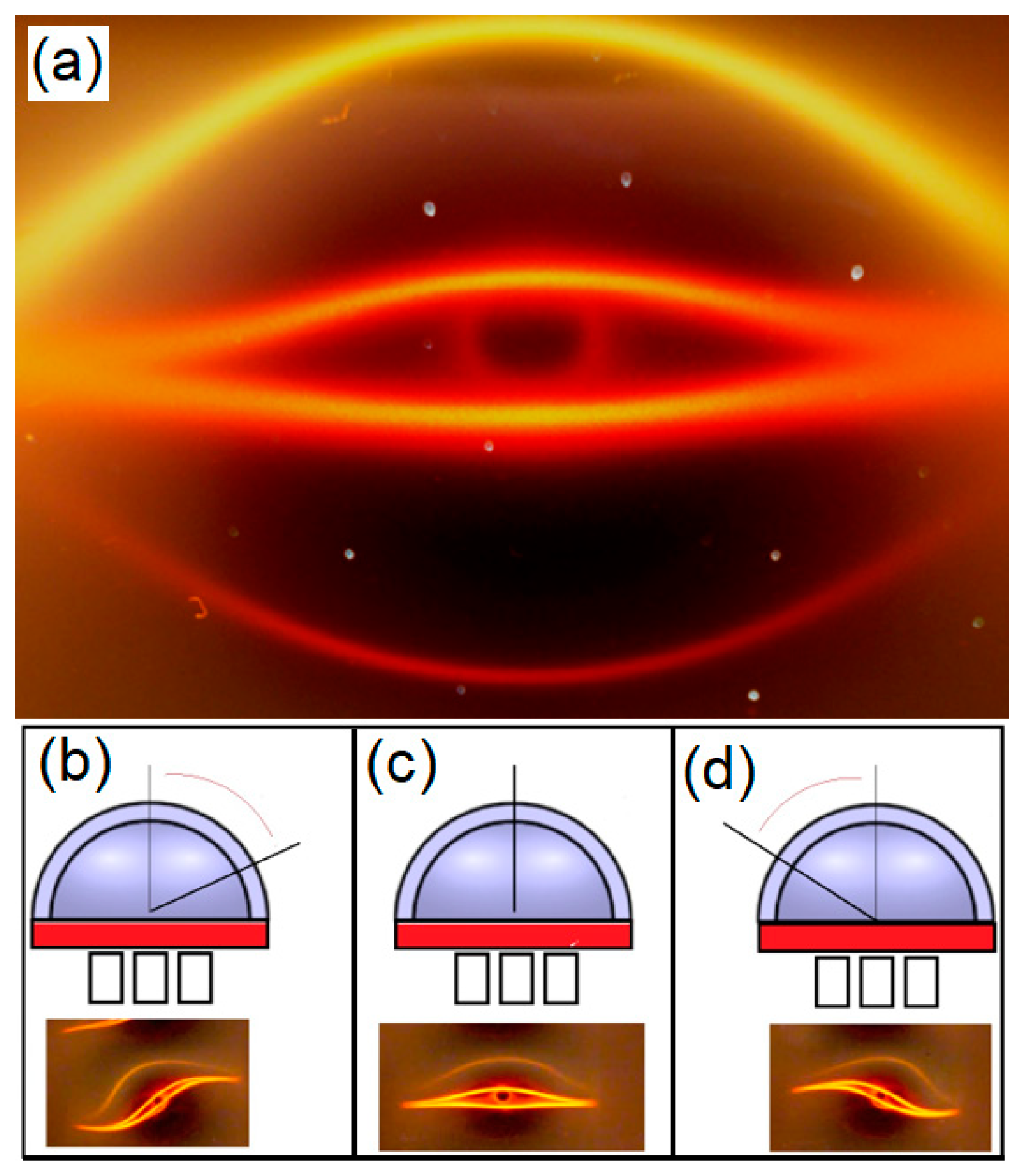
3.2. Light Patterns and Chirality

There is another interesting phenomenon associated with magnetochiral pattern of Figure 14, in which we have used three magnets to create this pattern, in a tripolar configuration south-north-south pole. Figure 14a is the top view of this pattern, and in Figure 14c, we can see the diagram of the experiment. For different angles of observation, this pattern suffers a distortion, as it is shown in the diagrams of Figure 14b,d. The image of Figure 14b is a reflection of Figure 14d, and it cannot be superposed to it. By definition, a system is chiral if it is distinguishable from its mirror image. A possible explanation for this effect could be the existence of magnetochiral assembly of nanoparticles affecting the light patterns. The ferrofluid undergoes structural transitions under external magnetic field, according to Singh et al. [12], because nanoscale particles could self-assemble into structures with unique spatial arrangements, such as helical-like structures due to the interplay of magnetic dipole-dipole and van der Walls interactions, as well as some entropic forces, depending on the geometry of the nanoparticles, leading to anisotropic effects. Even spherical particles may have angular dependences in their interactions if there is an internal direction defined within particles. The permanent magnetic dipole moment of the nanoparticles responds to an external magnetic field, and the interaction between ferromagnetic particles depends on the angle that the interparticle vector makes with the external field. The consequence of this anisotropy is the emergence of optical chiral structures. According to Witten [15], the dipolar interaction energy (E1,2) in a fluid of dipoles with magnetic moments μ1 and μ2 is given by
E 1 , 2 = r 3 [ μ 1 . μ 2 3 ( μ 1 . r ) ( μ 2 . r ) r 2 ] .
The strength of the dipolar interaction between particles may be expressed in terms of a dimensionless coupling constant l = Ed(i,j)/kbT, with kbT representing the thermal interaction. The dipolar interaction influences the organization of the rod structures at ambient temperatures, where l is close to 1. The magnetic perturbations twist the structure of nanoneedles, and this twist could be the source of this magnetochiral effect.

4. Results

Exploring Fixed Points and Trajectories with Magneto-Optics

We start comparing the space of phase of a pendulum at the top of Figure 15 with the diffracted lines at the bottom of Figure 15, with two centers and one saddle point in Figure 15. In the Ferrolens system, the attractors are represented by the set of diffracted lines. Another example of application is the evolution of the light pattern in Figure 16, from a limit cycle in (1), the separatrix is represented by the green line (2), and open trajectories (3) and (4), placing the magnet in the dipolar configuration. We have explored some magnets configurations and observed some attractors.
The key fact here is that we are observing in these images the information stored about the magnetic field, because just as the electric field can be expressed as a derivative of a scalar potential, so the magnetic field can be expressed as a derivative of the vector potential, and the diffraction properties of the ferrofluid connects these concepts and displays them directly in this optical effect. For example, the vector function of a limit cycle V of Figure 15 can be represented by:
V = y i ^ + x j ^ ,
where i and j are unit vectors in the plane x-y plane, with x = θ and y = dθ/dt. This function represents a circulation about the z axis perpendicular to this plane. Another useful function which represents a radial flow from some central point is the vector function V:
V = x i ^ + y j ^ .
The point at the center of this vector field is known as a ‘source’ in the context of dynamical systems theory because a source is a fixed point that repels a neighborhood, while a vector function pointing in the direction of its origin has a “sink.”
The vector function W of Figure 16 representing the limit cycle (1) corresponds to a not uniform magnetic field represented by the vector potential
W = V + λ V ,
with the coupling parameter λ. The complete diagram of the trajectories is presented in Figure 16a. In Figure 16b, there is a limit cycle with the label 1, in Figure 16c, the separatrix is represented by the green line in the diagram of Figure 16a with the label 2, and the other open trajectories with labels 3 and 4 are presented in Figure 16d,e respectively.
These examples are represented in two dimensions because the patterns observed in the Ferrolens is somehow the projection of the magnetic field in a plane, and locally we can use linear maps on R2 to represent the behavior of the system around some points, with the form
V A V = A ( x y ) = ( a 11 a 12 a 21 a 22 ) ( x y ) .
Using this representation, we can express the saddle point in the green line of Figure 16b with
A = ( a 0 0 b ) ,
with | a | > 1 > | b | , the successive points obtained by this map grows in the x-direction and shrinks in the y-direction.
The attractor obtained in Figure 17a gives us one example of the power of visualizing its structure, using this device. In this case, we are using three magnets in the tetrapolar configuration (Figure 4e), with a disc of white light as a light source. This source of non-collimated light is the white disc on the left, and the cylindrical magnets are placed at the right side, at the top, in a tetrapolar configuration. The trajectories escape from the white disc of light, passing close to the magnets, and they return to the white disc, closing the circuit, forming a ribbon of light. As we saw previously, the region close to the vicinity of a dipolar configuration can create a saddle point, in which the trajectories are attracted in one direction and repelled in another direction. In the tetrapolar configuration, we have at least two saddle points at each side of these three cylinders. This configuration develops the curved structure inside the attractor, and in this part of the attractor, the ribbon of light gives half a twist, like the case of a Möbius strip. In Figure 17b, we present a top view of this curved structure close to the magnets, where we can see the three magnets at the top, with the two saddle points and the light trajectories with a torsion at the center of the bottom part of this figure.

5. Conclusions

We have explored the possibility of creating some representations of dynamical systems using magnetic fields and optic fluidics. Our dynamical system is the direct observation of diffracted lines in the Ferrolens, a Hele-Shaw cell containing ferrofluid. This device is an interesting tool to visualize the abstract phase space directly, and it can help the community involved with dynamical systems to explore, teach and create some types of attractors.
The Ferrolens presents some curious properties involving the scattering of light partially confined in the plane of the ferrofluid, like a plane wave guide, as well as diffraction for the transmitted and reflected light when this system is subjected to an external magnetic field, suggesting the use of this device as a light modulator or display. The elliptical patterns are the result of a non-collimated light source placed behind the Ferrolens.
Although the comprehensive explanation of these diffracted lines is not something trivial, and still demands studies of the optical properties of light deflection by an ultra-thin film of nanoparticles, the light patterns obtained with this system are captivating, and using the analogy between different areas, the intellectual intersection of dynamical systems and electromagnetism can give us interesting results, such as the direct observation of magnetochiral effects.

Author Contributions

All authors contributed to prepare the experiments, propose the mechanisms involved, and analyze the results. The preparation of this manuscript was done mainly by A.T. and A.P.B.T.

Funding

This work was partially supported by Conselho Nacional de Desenvolvimento Científico e Tecnológico (CNPq), Instituto Nacional de Ciência e Tecnologia de Fluidos Complexos (INCT-FCx), and by Fundação de Amparo à Pesquisa do Estado de São Paulo (FAPESP) FAPES/CNPq#573560/2008-0.

Acknowledgments

A.T. and A.P.B.T. thanks to Conselho Nacional de Desenvolvimento Científico e Tecnológico (CNPq), Instituto Nacional de Ciência e Tecnologia de Fluidos Complexos (INCT-FCx), and by Fundação de Amparo à Pesquisa do Estado de São Paulo (FAPESP).

Conflicts of Interest

The authors declare no conflict of interest.

References

  1. Tufaile, A.; Sartorelli, J.C. Hénon-like attractor in air bubble formation. Phys. Lett. A 2000, 275, 211–217. [Google Scholar] [CrossRef]
  2. Tufaile, A.; Vanderelli, T.A.; Tufaile, A.P.B. Observing the Jumping Laser Dogs. J. Appl. Math. Phys. 2016, 4, 1977–1988. [Google Scholar] [CrossRef]
  3. Snyder, M.; Frederick, J. Photonic Dipole Contours of Ferrofluid Hele-Shaw Cell. Available online: http://www2.warwick.ac.uk/go/reinventionjournal/issues/volume2issue1/snyder (accessed on 24 February 2019).
  4. Scherer, C.; Neto, A.M.F. Ferrofluids, properties and applications. Braz. J. Phys. 2005, 35, 718–727. [Google Scholar] [CrossRef]
  5. Philip, J.; Laskar, J.M. Optical properties and applications of ferrofluids–A review. J. Nanofluids 2012, 1, 3–20. [Google Scholar] [CrossRef]
  6. Chiolerio, A.; Quadrelli, M.B. Smart Fluid Systems: The Advent of Autonomous Liquid Robotics. Adv. Sci. 2017, 4, 1700036. [Google Scholar] [CrossRef] [PubMed] [Green Version]
  7. Grossman, J.; McNeil, S. Nanotechnology in cancer medicine. Phys. Today 2012, 65, 38–42. [Google Scholar] [CrossRef]
  8. Yang, Z.; Wang, H.; Guo, P.; Ding, Y.; Lei, C.; Luo, Y. A multi-region magnetoimpedance-based bio-analytical system for ultrasensitive simultaneous determination of cardiac biomarkers myoglobin and C-reactive rprotein. Sensors 2018, 18, 1765. [Google Scholar] [CrossRef]
  9. Lin, J.F.; Tsao, Y.M.; Lee, M.Z. Measurement of birefringence and dichroism in magnetic fluids doped with nonmagnetic polystyrene microsphere. J. Jpn. Soc. Exp. Mech. 2013, 13, 13–17. [Google Scholar]
  10. Tufaile, A.; Vanderelli, T.A.; Tufaile, A.P.B. Light polarization using ferrofluids and magnetic fields. J. Adv. Condens. Matter. Phys. 2017, 2017, 2583717. [Google Scholar] [CrossRef]
  11. Rablau, C.; Vaishnava, P.; Sudakar, C. Magnetic-field-induced optical anisotropy in ferrofluids: A time-dependent light-scattering investigation. Phys. Rev. E 2008, 78, 051502. [Google Scholar] [CrossRef] [PubMed]
  12. Singh, G.; Chan, H.; Baskin, A.; Gelman, E.; Repnin, N.; Kral, P.; Klajn, R. Self-Assembly of magnetite nanocubes into helical superstructures. Science 2014, 345, 1149–1153. [Google Scholar] [CrossRef] [PubMed]
  13. Fowles, G.R. Introduction to modern optics, 2nd ed.; Dover: New York, NY, USA, 2013; pp. 108–110. ISBN 0-486-65957-7. [Google Scholar]
  14. Hubert, A.; Shäfer, R. Magnetic Domains: The Analysis of Magnetic Microstructures; Springer: Berlin, Germany, 1998; pp. 15–16. ISBN 978-3-540-64108-7. [Google Scholar]
  15. Witten, T.A.; Pincus, P.A. Structured Fluids, Polymers, Colloids, Surfactants, 1st ed.; Oxford University Press: Cary, NC, USA, 2004; ISBN 019958382X. [Google Scholar]
Figure 1. Magnetic contours observed in (a) using red light, and in (b) with green light for two distinct magnetic field configurations using the device Ferrolens.
Condensedmatter 04 00035 g001
Figure 2. Image of the magnetic contours obtained for a single cylindrical magnet in two orthogonal planes using the Ferrolens. In (a) the polar configuration is presented and in (b) the dipolar configuration, using LED ring lights providing radial illumination around the magnet. The diagram of the magnetic field generated by this magnet is presented in (c), with the previous images positioned in each respective orthogonal plane.
Condensedmatter 04 00035 g002
Figure 3. Illustrating a magneto-optic phenomenon in ferrofluids: approximation function for the optical response (the retardance in degrees) of the ferrofluid for different liquid concentrations, as a function of the magnetic field intensity. Besides the birefringence (retardance), the magnetic-optic phenomenon in ferrofluids is related to Faraday rotation, the Kerr effect, and linear dichroism.
Condensedmatter 04 00035 g003
Figure 4. Our source of the magnetic field in this experiment is based on permanent magnets, and we obtained directly the intensity of the magnetic field of permanent magnets using the gaussmeter. In (a), we obtained the magnetic field intensity for the polar configuration, and in (c) for the dipolar configuration, for the one-dimensional case. The magnetic field intensity obtained for the plane of the polar case is in (b), and for the dipolar case is in (d). In (e) a diagram of some magnet configurations are represented.
Condensedmatter 04 00035 g004
Figure 5. Light polarization observed in the Ferrolens for the polar configuration (a), using a cylindrical magnet with a length of 0.60 cm, and the diameter is 0.60 cm. In (b) simulation of light polarization using hyperbolic polynomials.
Condensedmatter 04 00035 g005
Figure 6. Light polarization observed in the Ferrolens for the dipolar configuration (a), using a neodymium cube magnet (0.5 × 0.5 × 0.5) cm. In (b) simulation of light polarization using hyperbolic polynomials.
Condensedmatter 04 00035 g006
Figure 7. Magnetic contours observed in Ferrolens using a tetrapolar configuration (a), using a cylindrical magnet with a length of 0.40 cm, and a diameter of 1.00 cm. Light polarization observed in the Ferrolens for the tetrapolar configuration (b), using a cylindrical magnet with a length of 0.60 cm, and a diameter of 0.60 cm. In (c) simulation of light polarization using hyperbolic polynomials.
Condensedmatter 04 00035 g007
Figure 8. Observing the needle-like structures of ferrofluids using an optical microscope (magnification of 2500 ×). These structures are formed by the nanoparticles in the presence of magnetic fields, ranging from 100 G to 500 G, creating these elongated structures.
Condensedmatter 04 00035 g008
Figure 9. Two light patterns obtained using a straight array of LEDs. In (a) for the case of polar configuration, and in (b) for dipolar configuration, using a cylindrical magnet with a length of 1.50 cm, and a diameter of 1.30 cm.
Condensedmatter 04 00035 g009
Figure 10. The pattern of curved lines from placing the straight line of LEDs far from the magnet in the dipolar configuration, using a cylindrical magnet with a length of 1.50 cm, and a diameter of 1.30 cm.
Condensedmatter 04 00035 g010
Figure 11. The general pattern of the orbits does not depend on the wavelength of the light source. The same pattern is observed for the dipolar configuration of Figure 9b for the color red in (a) and the color blue in (b), using a cylindrical magnet with a length of 1.50 cm, and a diameter of 1.30 cm.
Condensedmatter 04 00035 g011
Figure 12. Light diffraction phenomenon with collimated and uncollimated light observed simultaneously (a). The laser beam (coherent and collimated source of light) passing through the Ferrolens, while the formation of an elliptical light pattern in the plane of the Ferrolens is caused by light scattering of non-collimated light. The formation of patterns is a two-step process. This can be observed simultaneously in this figure, in which the first step is the diffraction of the green laser light through the Ferrolens in the presence of a magnetic field, projecting a curved line in the screen, with an intense light spot obtained due to the direct projection of the laser. The next step is obtained by the light spot of the laser hitting the screen, changing it to an uncollimated light source. In (b) a diagram illustrates this.
Condensedmatter 04 00035 g012
Figure 13. We have in this image a comparison between a simulation of magnetic potential and the experiment using Ferrolens with various light sources of different colors. In (a), the top view of the magnetic potential of three magnets with their paired poles, in (b) the same arrangement observed through the Ferrolens. The size of the neodymium cube magnets is 9.5 mm, and the ferrofluid layer is 6.0 mm above the magnets.
Condensedmatter 04 00035 g013
Figure 14. Magnetochiral effect. This set up has a bright incandescent lamp at 45 degrees incidence angle to the surface of the Ferrolens, and three identical cylinder magnets, in a south-north-south configuration. The north pole of a 12.7 mm diameter neodymium cylinder is directly under the Ferrolens, and we are presenting the light pattern of this central magnet in (a) and its respective diagram of observation in (c). For different angles of observation, this pattern suffers a distortion as shown in (b) and in (d).
Condensedmatter 04 00035 g014
Figure 15. Example of the analogy between the phase space of a pendulum and the diffracted lines obtained from our experiment, with two centers and one saddle point.
Condensedmatter 04 00035 g015
Figure 16. Trajectories observed in the polar configuration for the different points of view. The complete diagram of the trajectories is presented in (a). In (b) there is a limit cycle with the label 1, in (c) the separatrix is represented by the green line in the diagram with the label 2, and open trajectories with labels 3 and 4 are presented in (d) and (e), respectively.
Condensedmatter 04 00035 g016
Figure 17. Example of the structure of an attractor. The attractor obtained with a tetrapolar configuration is presented in (a). The trajectories scape from the white disc of light, passing close to the magnets, and they return to the white disc, closing the circuit, forming a ribbon of light. This configuration develops the curved structure inside the attractor, and in this part of the attractor, the ribbon of light gives half a twist, like the case of a Möbius strip. In (b) we present a top view of this curved structure close to the magnets.
Condensedmatter 04 00035 g017

