The Population Development of the Invasive Round Goby Neogobius melanostomus in Latvian Waters of the Baltic Sea

Abstract

The invasive round goby (Neogobius melanostomus) was established in the coastal waters of the Baltic Sea in the early 1990s. The first observation of the species in Latvian waters was in 2004. In the intervening period, the population grew, the species became of significance for local fisheries, and it likely impacted the local ecosystem in the Baltic Sea. In this study, we characterize the spatial–temporal population development of round goby in Latvian coastal waters using data from three different scientific and fisheries-independent surveys. We also include data from commercial fisheries landings to describe the fisheries targeting the species. Our results suggest an exponential increase in population numbers of round goby in Latvian waters, peaking in 2018, followed by a sharp decline. This observation is also supported by data from commercial fisheries landings. We suggest that intensive commercial fishing had a considerable impact on the rapid decline of the species, but that the decline was potentially amplified through a wider scale decline, as observed in many areas of the Baltic Sea. The results of this study contribute to the knowledge base on the species and how fisheries can aid in limiting the development of invasive fish populations. Based on the results of the study, we also provide recommendations for better future monitoring of the species in the coastal waters of the Baltic Sea.

1. Introduction

The origin of the round goby (hereafter RG) is the Ponto-Caspian region. The species was first recorded in the Baltic Sea near the Gulf of Gdansk in 1990 [1];by 1994, it was present in almost the whole of the Polish part of the Gulf of Gdansk [2]. Further range expansion of RG took place in the German Rugen area and the Polish part of the Vistula Lagoon in 1999; by 2005, the species was found in Lithuanian coastal waters, later being observed in the Gulf of Riga, as well as in the Gulf of Finland in the 2000s. In the 2010s, RG was first observed on the islands of Gotland and Åland (central Baltic Sea), in the Kattegat, and along the Swedish coastline [3]. Currently, the species is found in all sub-basins of the Baltic Sea [4]. The population expansion is not surprising, considering that the low biodiversity and available niches of the Baltic Sea ecosystem make the invasion of any brackish water invasive species highly likely and probably successful [5]. The invasion and range expansion of the species is also significantly promoted by the high shipping activity in the Baltic Sea, which serves as a vector for dispersal, and peculiarities of the Baltic Sea hydrology, with low wave exposure and bottom currents both being factors that favor round goby establishment [6]. The latest climate models predict an increase in water temperatures in the Baltic Sea region [7], something that also likely favors a further range expansion of the species, as increasing temperatures may increase the duration of its spawning period [8,9]. As a result of the rapid population expansion, RG is considered one of the most invasive non-indigenous species in the Baltic Sea to date [10].

Dispersal of RG occurs in two life stages. The key vector for long-distance dispersal is the ballast waters of ships that transport juvenile RGs and fertilized eggs between ports. Local dispersal is mediated via a combination of natural range expansion and additional anthropogenic transport mechanisms, such as small boat shipping and canals [11]. The dispersal rate of RG in the Baltic Sea is approximately 30 km per year [12].

The ecological role of RG in the Baltic Sea is both as a mesopredator and a prey for higher trophic-level organisms. RG feeds on benthic invertebrates, and with increasing body size, the prey composition gradually shifts from decapods to mollusks and small fish [13,14,15]. Fish species such as cod (Gadus morhua), pikeperch (Sander lucioperca), European perch (Perca fluviatilis), and turbot (Scophthalmus maximus) prey on RG [16,17,18,19]. RG is also found in the diet of birds, such as greater cormorants (Phalacrocorax carbo) and grey herons (Ardea cinerea), as well as mammals, such as grey seals (Halichoerus grypus) [20,21,22]. RG does, therefore, likely have an impact on the Baltic Sea ecosystem and local food webs by competing for food with native species [13,22,23,24,25], as well as by facilitating novel energetic pathways from benthic organisms to top predators [10,16]. In another system that was invaded by RG—Lake Huron—there is evidence that the species benefitted from climatic regime shift that also coincided with a decrease in fish species richness [26].

RG was first recorded in Latvian coastal waters in 2004; in the intervening period the population grew. The coastal area in the southwest part of the Latvian exclusive economic zone waters (EEZw) could hold one of the highest RG concentrations in the Baltic Sea. Subsequently, local fisheries started to target the species, and the area is also likely the location with the highest commercial landings of the species in the Baltic Sea [13]. There is a general lack of coordinated monitoring programs for the species, and the quantification of the actual abundance of the species is, therefore, often missing [4,27].

In this study, the overall aim is to describe the population development and range expansion of RG in Latvian waters using fisheries-independent monitoring data and commercial fisheries landings. This analysis is performed by first developing calibration coefficients between the different monitoring gears used and utilizing available data sources. Following this step, we describe the observed population development of the species in a spatial–temporal context. Finally, we create a population change model using the TRIM tool [28], which is widely used in wildlife monitoring data analysis but is overlooked as a monitoring tool in fisheries. We also suggest an outline for future monitoring of the species in the Baltic Sea.

2. Materials and Methods

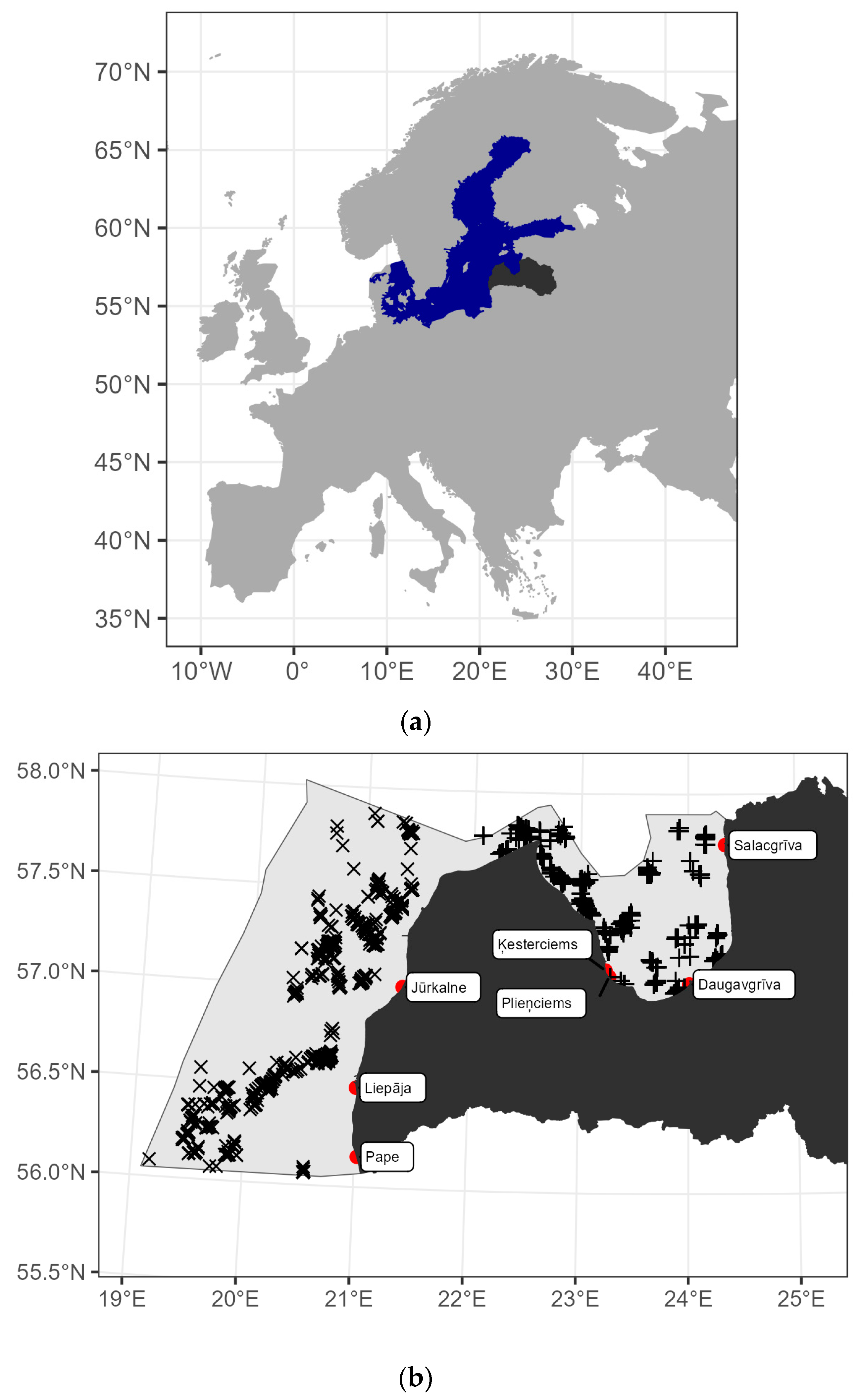
2.1. Study Area and Methods

Latvia is a Northern European country bordering the Baltic Sea (Figure 1a,b). Its EEZ contains parts of the Eastern Gotland sub-basin (hereafter referred to as the open sea) and the Gulf of Riga (Figure 1b). In the open sea, the salinity varies between 7 and 12%, though in the Gulf of Riga, it is substantially lower (3–7‰). The average depth of the Gulf of Riga is 26 m, while the average depth of the Eastern Gotland sub-basin is 55 m [29].

2.2. Fish Monitoring Methods

Given the differences in the geomorphological and hydrological properties of the Latvian EEZ, fish monitoring was performed with three different methods: (1) coastal fish monitoring (CFM), (2) bottom trawling in the Gulf of Riga (GORDEM), and (3) bottom trawling in the open sea as a part of the Baltic international benthic trawl survey (BITS) (Figure 1b).

2.2.1. Latvian National Coastal Fish Monitoring (CFM)

The CFM began in 1995 with the standard “Coastal net series” (hereinafter, Coastal nets), though from 2016, the gear “Nordic Coastal Multi-mesh Survey Nets“(hereinafter, Nordic nets) was exclusively used in monitoring. The Nordic nets are widespread standard fish monitoring gear used in the Baltic Sea [30] that consist of nine 5 meter-long panels with mesh sizes in order 30; 15; 38; 10; 48; 12; 24; 60; 19 mm, the linen of which is made of nylon monofilament twine. The Coastal nets linen is made of multifilament twine (“kapron” or “nylon-6”) and has six 30 meter-long panels with mesh sizes in order 17; 22; 25; 30; 33; 38 mm. From 2014 to 2016, both gears were used in parallel to enable the calibration of catches across gears (see Section 2.3 for additional details).

Monitoring was conducted monthly (except in January) with both gears in seven coastal areas (Figure 1b) at fixed stations in 3–5 m water depth. The total number, weight, and length distributions of all fish species captured were recorded from every station. The number of individual stations and the distance between them were chosen according to the Baltic Marine Environment Protection Commission (HELCOM) guidelines for coastal fish monitoring [30].

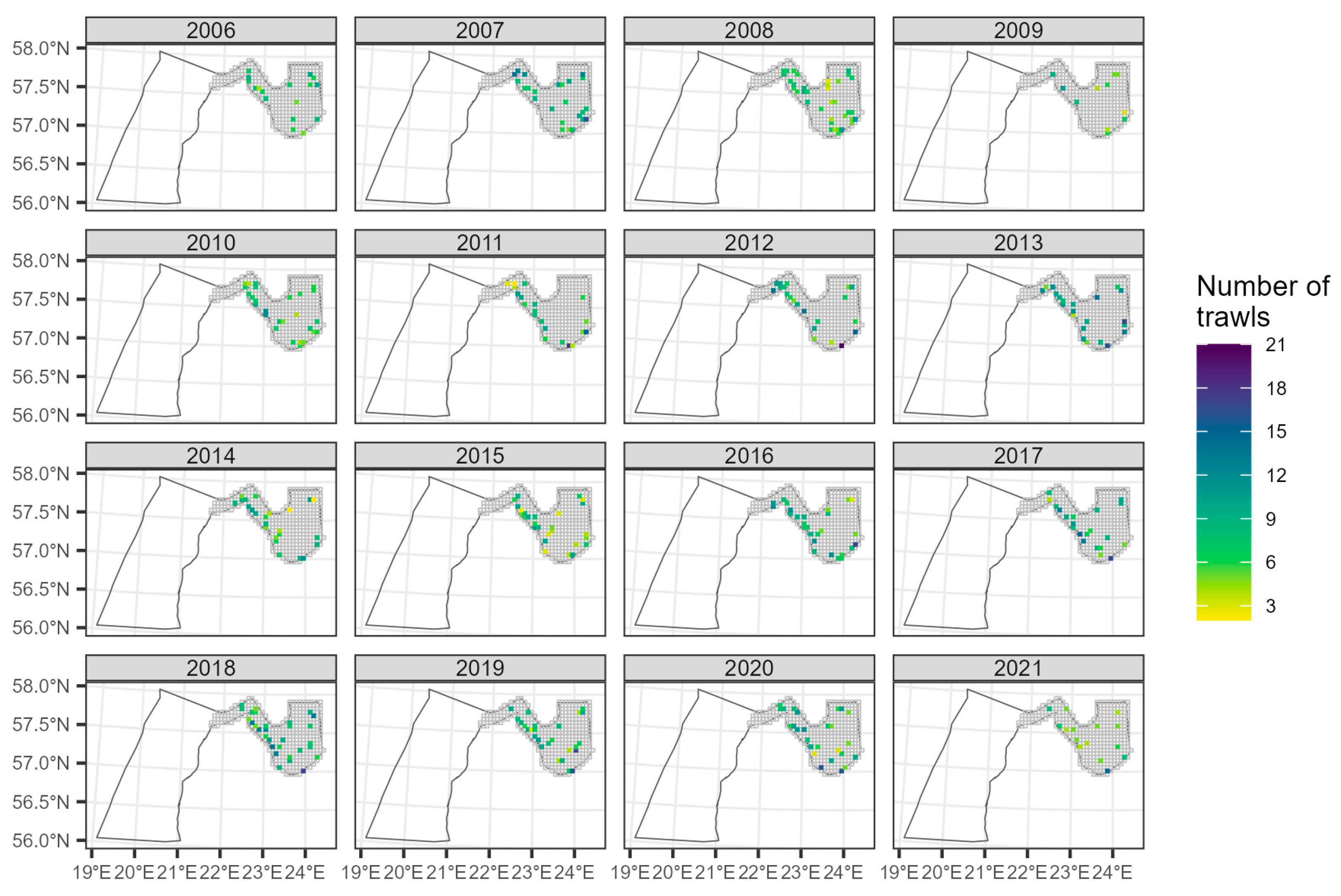
2.2.2. Latvian National Benthic Trawl Surveys in the Gulf of Riga (GORDEM)

The survey is performed three times per year, in May, August, and October, in the Gulf of Riga (ICES Sub-division 28.1, Figure 1b). Trawling is performed during daylight and night-time with a special demersal trawl that is 18 m wide and 1.5 m high and a mesh size that ranges from 17 mm to 6 mm in the codend. Fish sampling follows the method of the BITS survey described below.

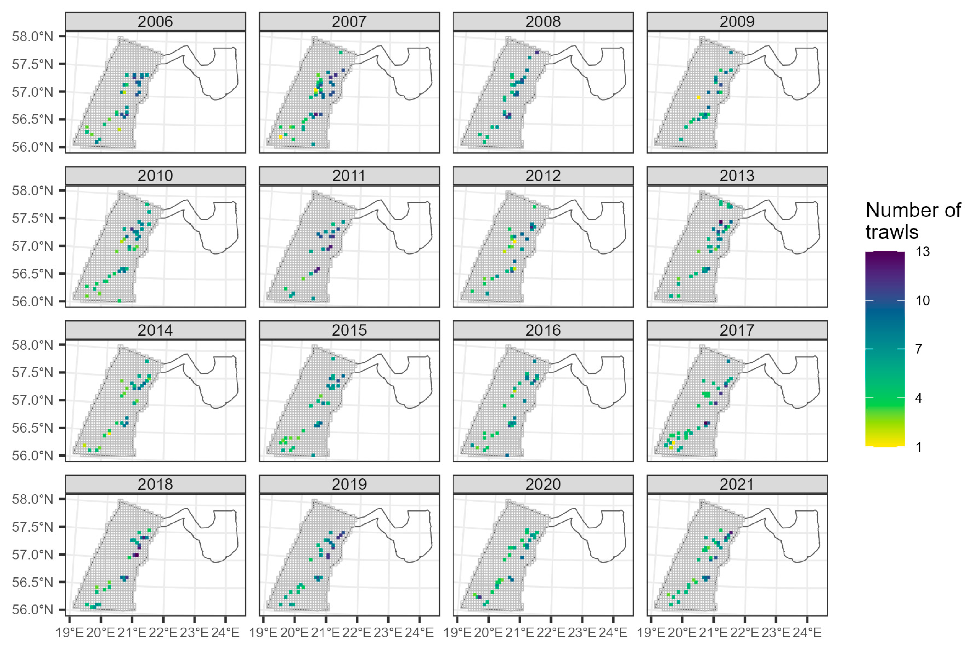
2.2.3. Baltic International Benthic Trawl Survey (BITS)

The surveys were conducted in March and December in the open sea area of Latvian waters. The primary purpose of the survey is to produce abundance estimates and indices of recruitment for cod and flounder (Platichthys flesus) in the Eastern Baltic Sea (ICES Sub-divisions 25–32). The survey had a random stratified design, with catch stations selected from a set of known trawlable sites [31]. The total number, weight, and length distributions were recorded for all fish species from every trawling station in the survey. Besides biological measurements, detailed information on the hauling sites and environmental parameters were recorded according to the international protocol [31].

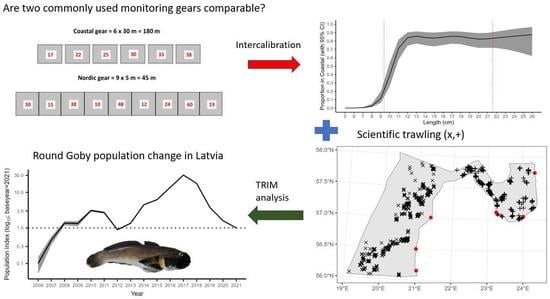
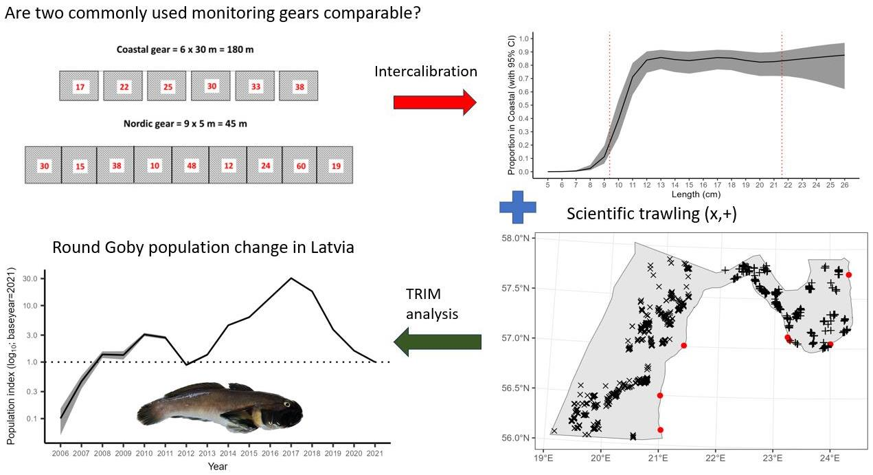
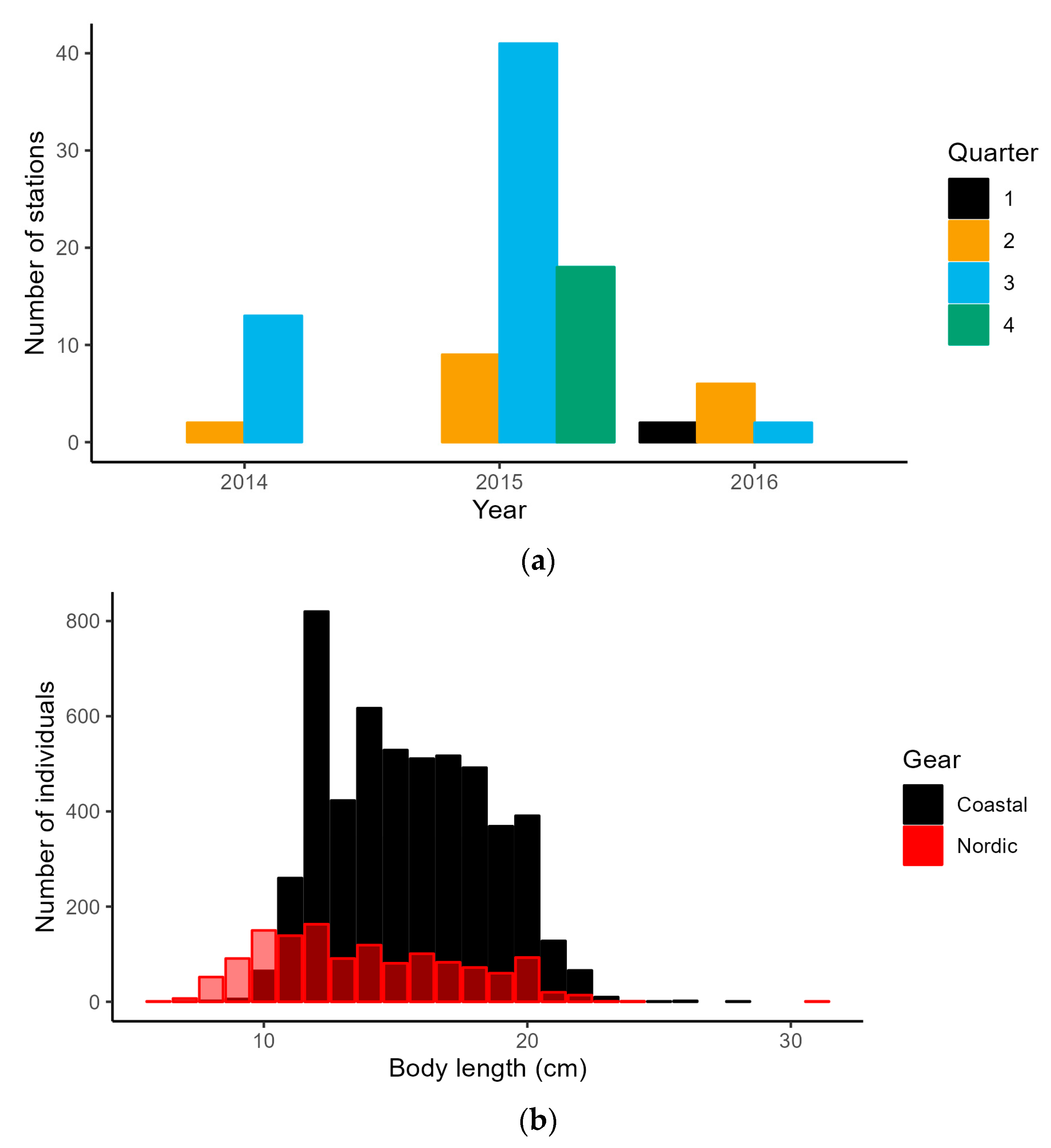
2.3. CFM Gear Calibration

For calibrating the catches between the two gears used in coastal fish monitoring (“Nordic nets” and “Coastal nets”), the seven coastal sites (red dots in Figure 1b) were used simultaneously in 2014–2016. Both gears were tied together with a 100m rope, providing a paired sampling design. The number of monitoring stations available for analysis per seasonal quarter per year is shown in Figure 2a.

The paired design allowed analysis of binomial data (i.e., the probability that individuals were captured in one of the gears, given the number of individuals captured in the other gear). To obtain comparable estimates of RG catches across gears, we aggregated the number of individuals per 1 cm length group (from min = 5 cm to max = 31 cm) per gear in every fishing occasion at the station level. Given the mesh sizes (see Section 2.2.1) for the gears used, it was expected that smaller fish may be less representatively captured than the larger fish. Therefore, in gillnets, it is often accepted to focus the analysis on fish larger than 12 cm in length [32]. To describe the abundance of individuals per gear at length (Figure 2b), we used 1 cm length classes for individuals above 10 cm, and calculated weighted (by count) mean body length in groups of smaller fish. Due to the small number of individuals captured, we used the same weighted mean size calculation for fish larger than 21 cm (Figure 2b). Thus, by obtaining length as a semi-quantity, which was usable as an independent variable, a gear-specific catchability was expected to change with fish size (Figure 2b).

We assumed a binomial response to defining catchability in the “Coastal nets”, given the number of RG captured in the “Nordic nets”, and assuming a non-linear effect of body length on the gear-specific catchability. To model these assumptions, we used generalized additive modeling (GAM) with a binomial family distribution and a logistic link function [33]. We used these parameters (and their interactions) as random variables controlling imbalance in data (Figure 2a), as well as a hierarchical design. We evaluated six different random variable structures for their variance, and excluded models with zero variance from further analysis. This approach resulted in models with a random intercept for Area (1), Station (2), and Quarter (3), as well as a hierarchical structure for the station within Area (4). We employed the second-order Akaike information criterion (AICc) in model evaluation, selecting the model with the lowest AICc value as the best [34]. All models had the same fixed part, with six thin plate spline basis functions accounting for non-linearity in gear-specific catchability over body length. We utilized the R [35] packages gamm4 [36] and mgcv [37] in modeling and ecosystem tidyverse [38] in data processing and visualizations.

We used our best model to predict the proportion (with 95% confidence intervals) of RG individuals captured in “Coastal nets” per every 1 cm from 5 to 26 cm, and calculated the odds ratio. We suggested the use of the odds ratio as a multiplicative value for the recalculation of the number of individuals in one gear, given the value in another [39]. When recalculating from “Nordic nets” to “Coastal nets” this value was used as a multiplicator of the observed number of fish. The intercalibrated data were used in further population change analyses.

2.4. Population Change Analysis

To address temporal changes in the RG population surveyed, we used the TRIM tool [28]. This tool allowed a combination of trends obtained through different and directly incomparable methods [40]. Firstly, the TRIM tool calculated yearly indices reflecting the population size relative to a base year. Typically, yearly indices were calculated from one value per monitoring site and year, including an imputation procedure when missing values occur. In case of multiple counts at site and year, the use of maximum value was suggested [28] and used. In addition, if every site has multiple counts per year at different months, this fact can be incorporated to better account for seasonality. Finally, population trends obtained via different monitoring methods can be combined using model variance–covariance matrices, avoiding possible effects of different monitored population sizes [41]. The set of tools is open access and implemented in R (R Core Team, 2022) package rtrim [42]. We only included sites where RG was observed for at least two years.

2.4.1. Coastal Fish Monitoring Data Preprocessing

We rounded non-integer values to an integer necessary for TRIM analysis, and we expect no effect on the result as Pearson’s correlation coefficient is near-functional (r > 0.999, t = 7081.1, df = 5875, p < 0.001).

A total of 42 stations distributed within seven areas were included in the Latvian coastal monitoring program. The remaining stations were surveyed on 1734 occasions, sometimes being surveyed more than once per month. Accounting for the maximum number of fishing occasions per site and month resulted in 1141 data points being found for the analysis. The number of stations monitored per area in the year is shown in Figure 3.

2.4.2. BITS and GORDEM Data Preprocessing

In contrast to coastal monitoring, trawl stations impacted by to weather conditions could not always be located with high precision during the surveys. Therefore, we used the starting coordinates of monitoring stations to spatially join with a 5 × 5 km rectangular grid (coordinate reference system epsg: 3059) covering the Latvian EEZ. The grid cell size approximately matched the daily migration of the RG, considering a maximum migration range of 10 km during the spawning season [20]. We treated observations from the same grid cell as replicates.

A total of 105 grid cells (5 km) were monitored in the open sea (Appendix A, Figure A1). However, 27 grid cells had observations from only one year and were excluded from the analysis. In total, these cells were surveyed on 409 occasions, with each cell surveyed no more than once per month. Even though the RG had been observed since 2010, these sites did not have a second monitoring occasion in the upcoming years. Due to this restriction, we could only perform analysis on data found since 2015 at 258 monitoring occasions. Of those monitoring sites, 59 did not have any observation of the species at any time point; therefore, these sites were excluded.

A total of 78 grid cells (5 km) were monitored in the Gulf of Riga with the GORDEM scheme (Appendix A, Figure A2). In total, 30 of the grid cells had observations from only one year and were, thus, excluded from the analysis. Together, the cells were summarized on 361 occasions, with each location summarized no more than once per month. Seven monitoring sites did not have any observation of the species at any time point; therefore, these sites were excluded.

2.4.3. Standardization across Surveys

Even though it is stated that the speed and length of trawling were constant across methods, in practice, this may not be true. Therefore, we standardized counts (number of individuals captured per trawling occasion) before further analysis.

In the GORDEM survey, considering a constant trawling speed (3 knots), the actual hauling time no more than 30 min. Therefore, we standardized the catch to 1 trawling/hour using a formula (Equation (1)), where

one trawling hour = (number of individuals)/(hauling time in minutes) × 60.

(1)

We standardized the BITS counts to a 10-hectare trawled area. For standardization, we selected only hauls with a hauling time of at least 15 min and observations with the trawl type “TVL”. We assumed the ground speed to be three knots, unless registered in the International Council of the Exploration of The Sea (ICES) database DATRAS. We assumed the horizontal opening to be 32 m [43]. Therefore, we could apply the formula (Equation (2)).

$$\begin{array}{c}\text{standardized value = (count from database)/((speed from database) × a ×}\\ \text{(duration from database) × c)/d) × e,}\end{array}$$

(2)

where a is 1.852/60 × 1000 to convert knots to meters per minute; c is trawling horizontal opening; d is 10,000 to convert to ha, and e is 10 to convert to 10 ha. If, per any census occasion, the species was not recorded, we assumed the count to be 0.

Standardization of counts led to non-integer values; therefore, we rounded the result to the integer, which was necessary for TRIM analysis. We expected this rounding to have no effect on the analysis results, as Pearson’s correlation coefficients imply functional (r = 1, t = 215,727, df = 359, p < 0.001) or near-functional (r = 0.99, t = 23,711, df = 443, p < 0.001) correlation at GORDEM and BITS data, respectively.

2.4.4. Population Model

Before we performed population change analysis, we used Pearson’s correlation analysis to estimate the possible error introduced by rounding standardized counts to integers. In every case, the result was near-functional correlation; therefore, we continued with the population change analysis.

We employed TRIM analysis of monthly data, allowing independent slopes over time per site (model = 3) (for a full explanation, see [40]). This model generally could be written as a formula (Equation (3))

lnμijm = αi + βj + δm,

(3)

where μ_ijm is an expected count, α_i is a population size parameter for the site i, and β_j is a time point parameter for year j, with the δ_m being month parameters for month m (for a full explanation, see [40]). We created a separate model per monitoring scheme, as their observed counts and standardization procedures were very different.

To ease the readability of the results from different monitoring schemes, we used 2021 as a plot baseline. Therefore, the yearly indices were population sizes relative to those of 2021.

2.4.5. Trend Combination

Finally, we used the results of the monitoring scheme-specific analysis computed as the time totals and variance–covariance matrices of each monitoring scheme-specific model in stratified sampling analysis. Essentially, this analysis was the same TRIM model = 3, albeit without the parameters for month (δ_m in the previous equation). The main difference was that we did not use site-level information, instead using already calculated time totals per stratum defined by the monitoring scheme. Thus, the equation could be written as a formula (Equation (4))

lnμij = θi + βj,

(4)

where μ_ij is an expected count, θ_i is a stratum parameter for monitoring scheme i, and β_j is a time point parameter for year j (for a full explanation see [40]). The relationships between time points within the monitoring scheme are described via variance–covariance matrices, which were analyzed to obtain results at the super-stratum (super-population) level (for a full explanation, see [40]).

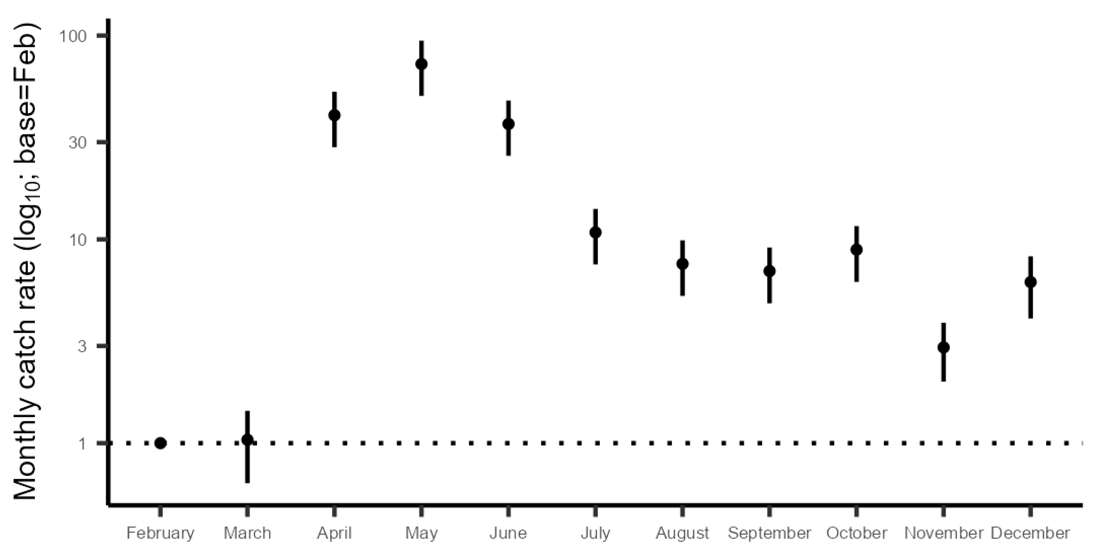
2.4.6. Monthly Catch Rates

To provide evidence of the seasonal differences in catch rates of RG, we extracted monthly catch rates from the coastal fish monitoring population model. This model was the only scheme that provided information on a monthly basis; therefore, we did not repeat the procedure on other models.

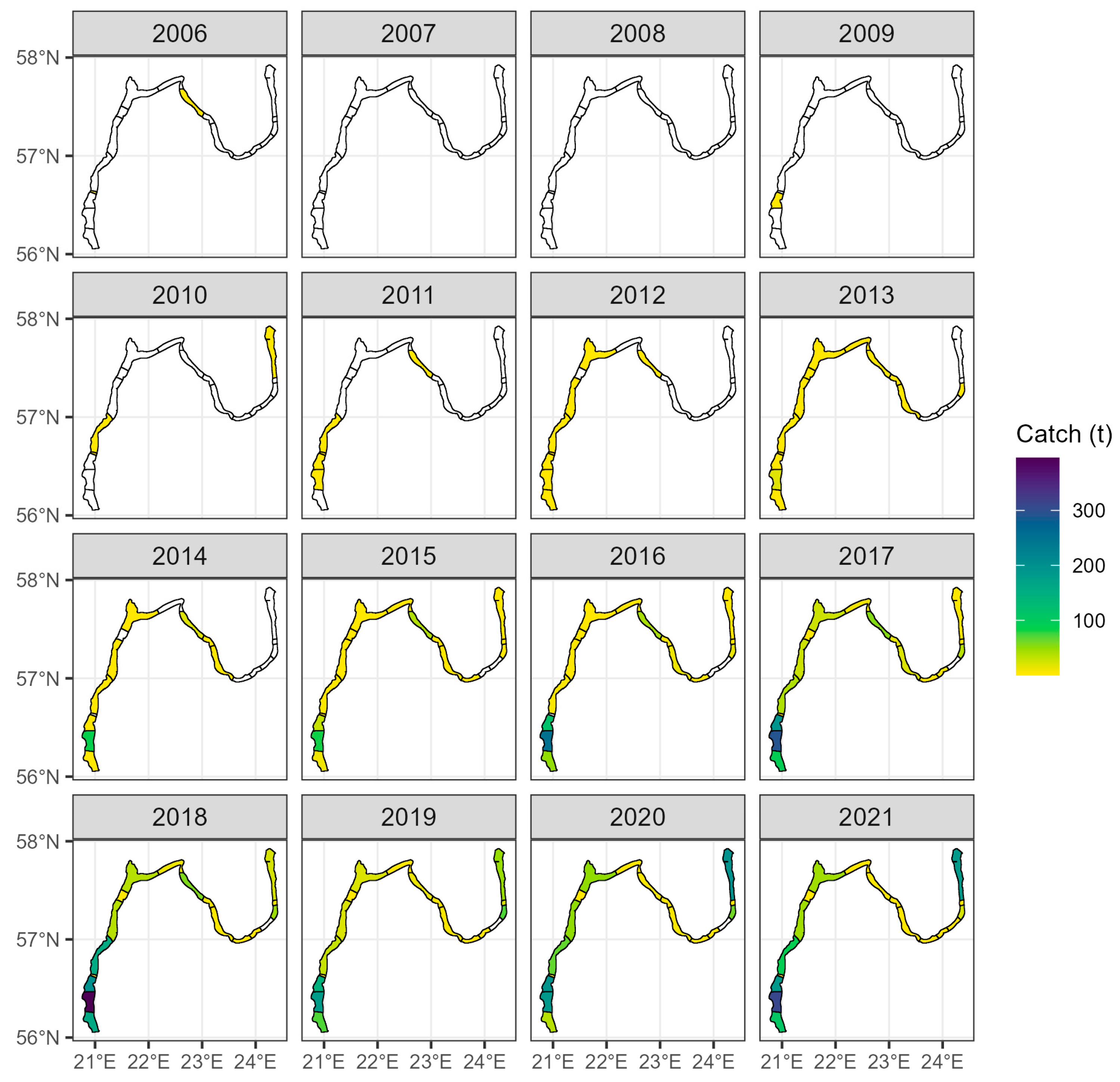
2.5. Commercial Fisheries Data

Data were extracted from Latvian coastal fishery logbooks from 2005 to 2021. This approach did not allow for the development of mathematically correct calculations, and the approximate general indicators that could be obtained did not allow further detailed analysis. We, therefore, only visualized and described the landings within the limits of total annual values in regional municipalities.

3. Results

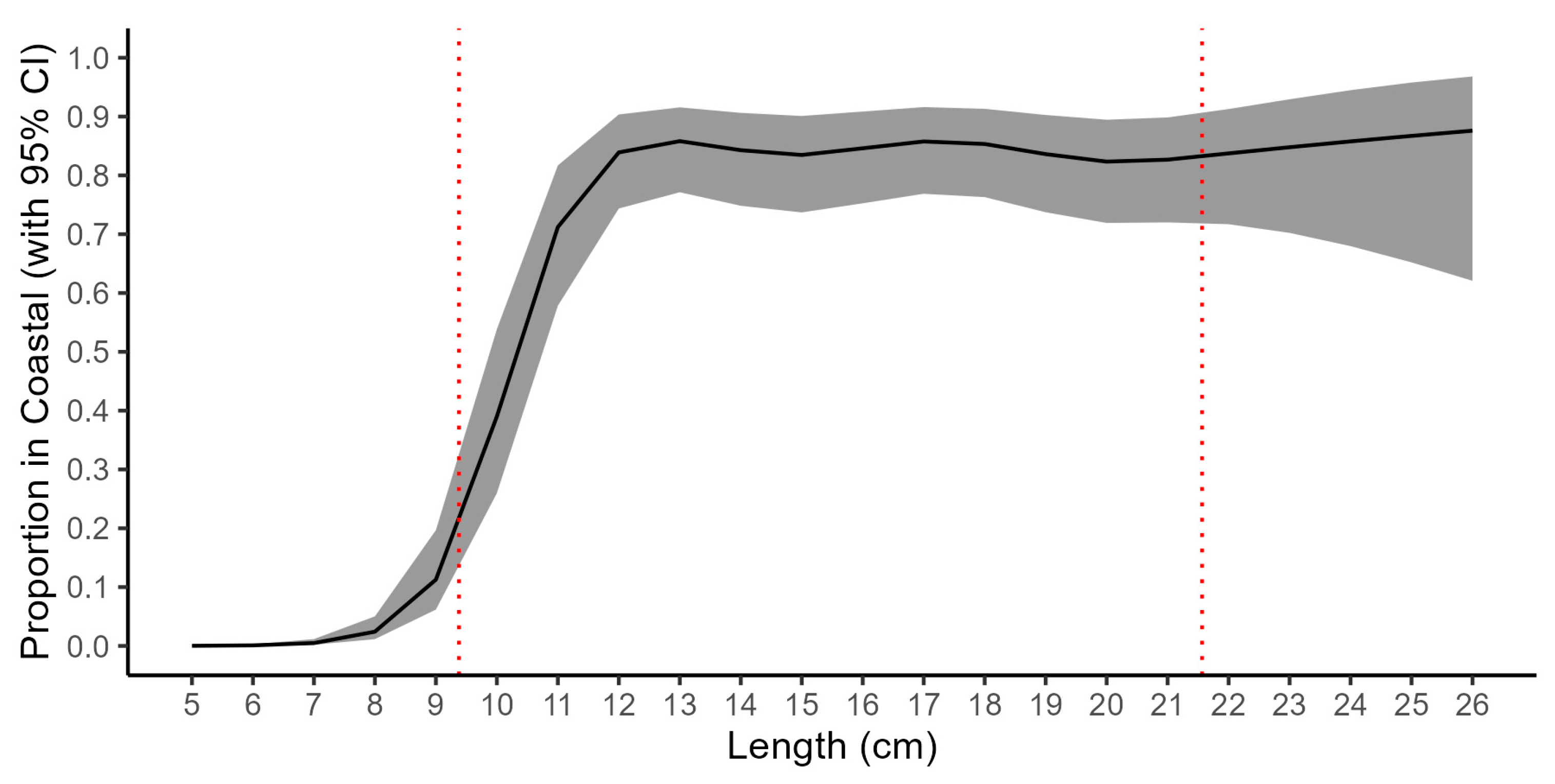
3.1. Coastal Fish Monitoring Gear Calibration

From seven possible combinations of the random effects (including the baseline model), three examples could not be further used due to zero variance. These examples were models with hierarchical sampling designs including seasonal quarters, suggesting no reasonable effect in the differences between seasons. We found the model with a random intercept for monitoring area to be the best performing model based on AICc (

Table 1. Model selection table (AICc = second order Akaike-information criterion values; _marginalR² = marginal pseudo-determination coefficients; _conditionalR² = conditional pseudo-determination coefficients; ICC = intraclass correlation coefficient).

Random Effects Used	AICc	marginalR2	conditionalR2	ICC
Baseline (no random effects)	1356.268	0.582	-	-
1|Area	1299.265	0.723	0.752	0.106
1|Quarter	1355.696	0.703	0.709	0.020
1|Station	1307.899	0.723	0.749	0.092
1|Area/Station	1309.917	0.722	0.752	0.107

). This model has a relatively high ability to describe data, with its pseudo-determination coefficients being above 70%.

Every random effect model converged to the fifth order polynomial (edf = 4.891, ref. df = 4.891, Chi-square = 538, p-value < 0.001 in the best model) with strong catchability preference in “Nordic nets” for small fish (see Figure 4), followed by the steep change in preference towards “Coastal nets” from 12 cm. Catchability, beginning with fish body length values of 12 cm, can be considered relatively stable (within confidence interval), being approximately 5.35 times higher in “Coastal nets” than in “Nordic nets” (Figure 4, Appendix B,

Table A1. Recalculation (from “Nordic” to “Coastal”) coefficients and their 95% confidence intervals.

Length (cm)	Proportion in “Coastal”	Proportion in “Coastal” (95%CI)		Multiplicator for “Nordic” (to Obtain Values at “Coastal”)	Multiplicator (95%CI)
5	0.0002	0.0001	0.0006	0.0002	0.0001	0.0006
6	0.0009	0.0003	0.0027	0.0009	0.0003	0.0027
7	0.0048	0.0020	0.0116	0.0048	0.0020	0.0118
8	0.0242	0.0115	0.0503	0.0248	0.0116	0.0529
9	0.1127	0.0617	0.1968	0.1270	0.0658	0.2451
10	0.3901	0.2597	0.5385	0.6397	0.3508	1.1666
11	0.7121	0.5783	0.8169	2.4734	1.3713	4.4612
12	0.8391	0.7437	0.9036	5.2138	2.9012	9.3699
13	0.8582	0.7713	0.9156	6.0506	3.3725	10.8554
14	0.8428	0.7483	0.9063	5.3620	2.9729	9.6712
15	0.8347	0.7370	0.9010	5.0503	2.8022	9.1022
16	0.8460	0.7525	0.9085	5.4953	3.0405	9.9319
17	0.8576	0.7687	0.9161	6.0249	3.3236	10.9215
18	0.8534	0.7630	0.9132	5.8203	3.2201	10.5201
19	0.8361	0.7373	0.9027	5.1028	2.8069	9.2769
20	0.8234	0.7191	0.8946	4.6618	2.5599	8.4897
21	0.8267	0.7200	0.8985	4.7711	2.5718	8.8514
22	0.8374	0.7170	0.9128	5.1491	2.5334	10.4654
23	0.8478	0.7022	0.9294	5.5724	2.3583	13.1670
24	0.8578	0.6797	0.9449	6.0304	2.1223	17.1355
25	0.8671	0.6521	0.9579	6.5261	1.8741	22.7255
26	0.8760	0.6208	0.9682	7.0626	1.6368	30.4736

). As the “Coastal nets” are 180 m long, while the “Nordic nets” are 45 m, this results makes a size ratio of 4, which is lower than the observed proportion (>5 timers at sizes ≥12 cm), hence indicating catchability preference. This gear length ratio is, however, well within the confidence interval of correction values, as shown in Appendix B, Table A1.

Recalculation coefficients and their 95% confidence intervals for “Nordic nets” from “Coastal nets” are given in Appendix B, Table A1, along with predicted probabilities (as shown in Figure 4) and their confidence intervals. Even though confidence intervals seem reasonable, we suggest a cautious use of the correction values in individuals smaller than 9 cm or larger than 22 cm due to the scarcity of data available for modeling (Figure 2b).

3.2. Population Development of the RG

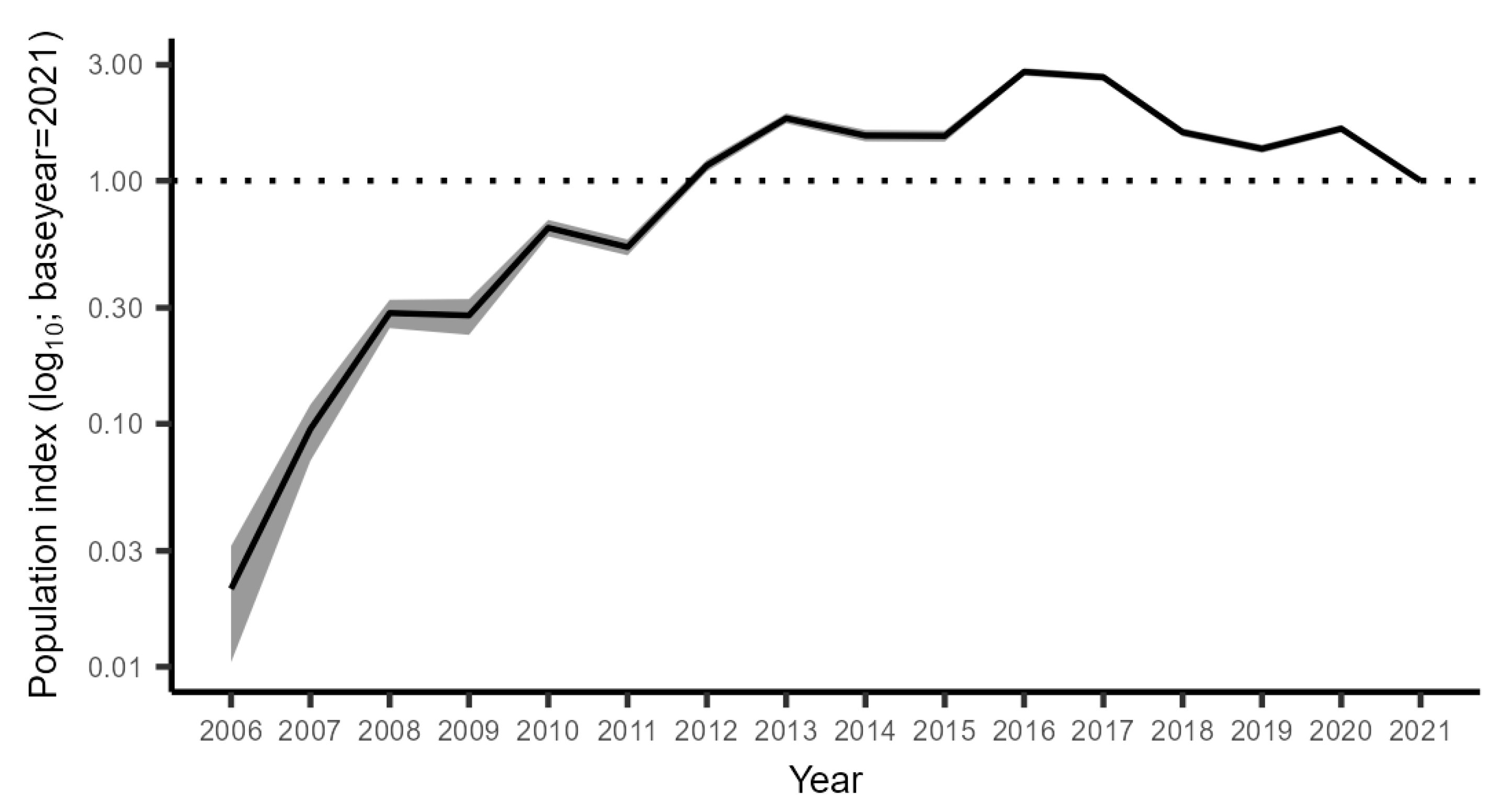
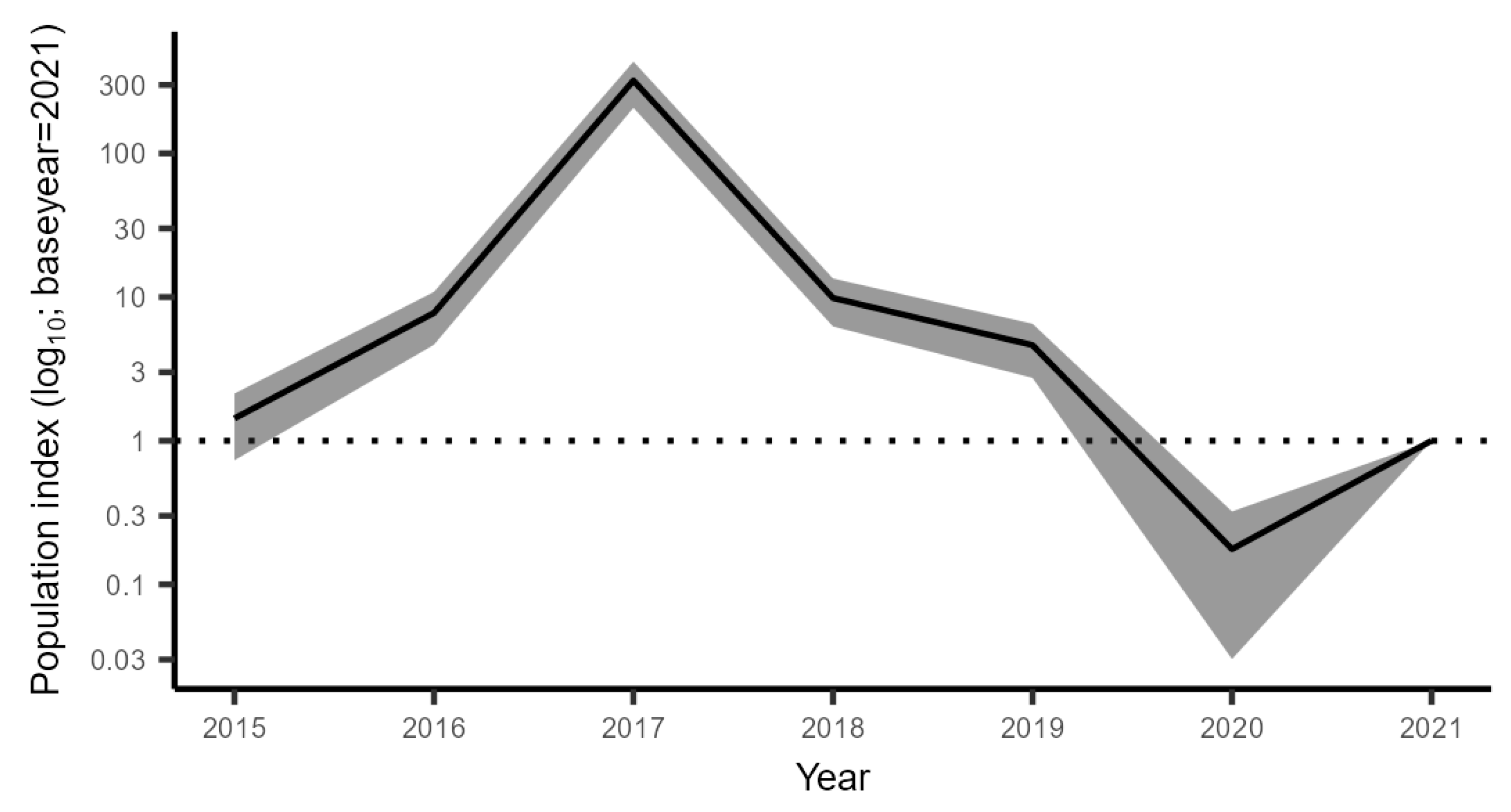
3.2.1. The Trend in the CFM

The first record of RG in CFM was noted in 2006. In the intervening years, the species was caught every year in increasing quantities. The TRIM analysis of the coastal fish monitoring data suggests a strong overall increase (p < 0.001) in population densities, with an annual rate of increase of 1.24 (±0.016 S.E.). However, the population development was not monotonic (Figure 5), as a strong increase between 2006 and 2017 was followed by a decline. The peak of the population size occurred in 2016–2017, when the population was approximately 3 times larger than it was in 2021.

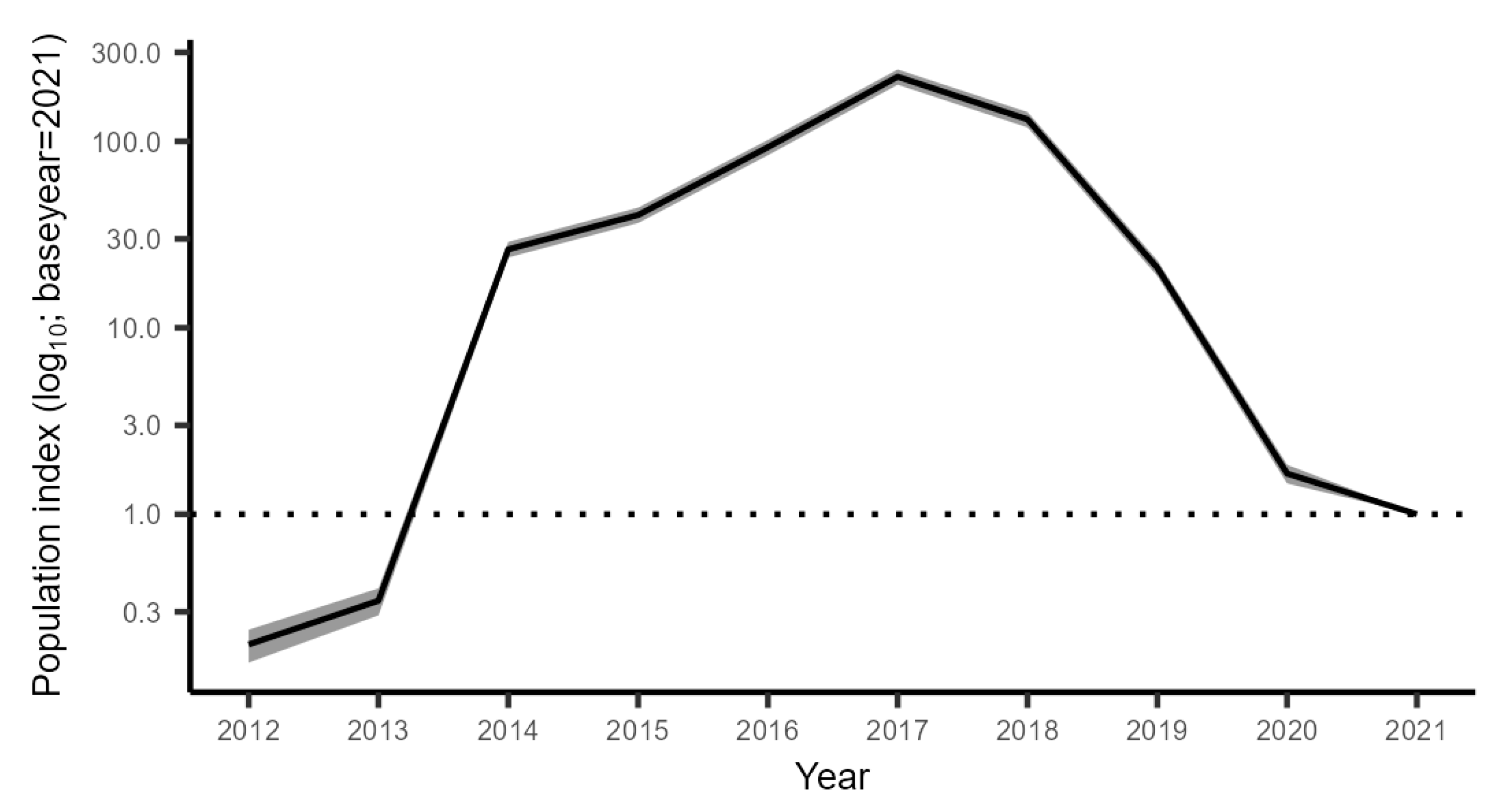
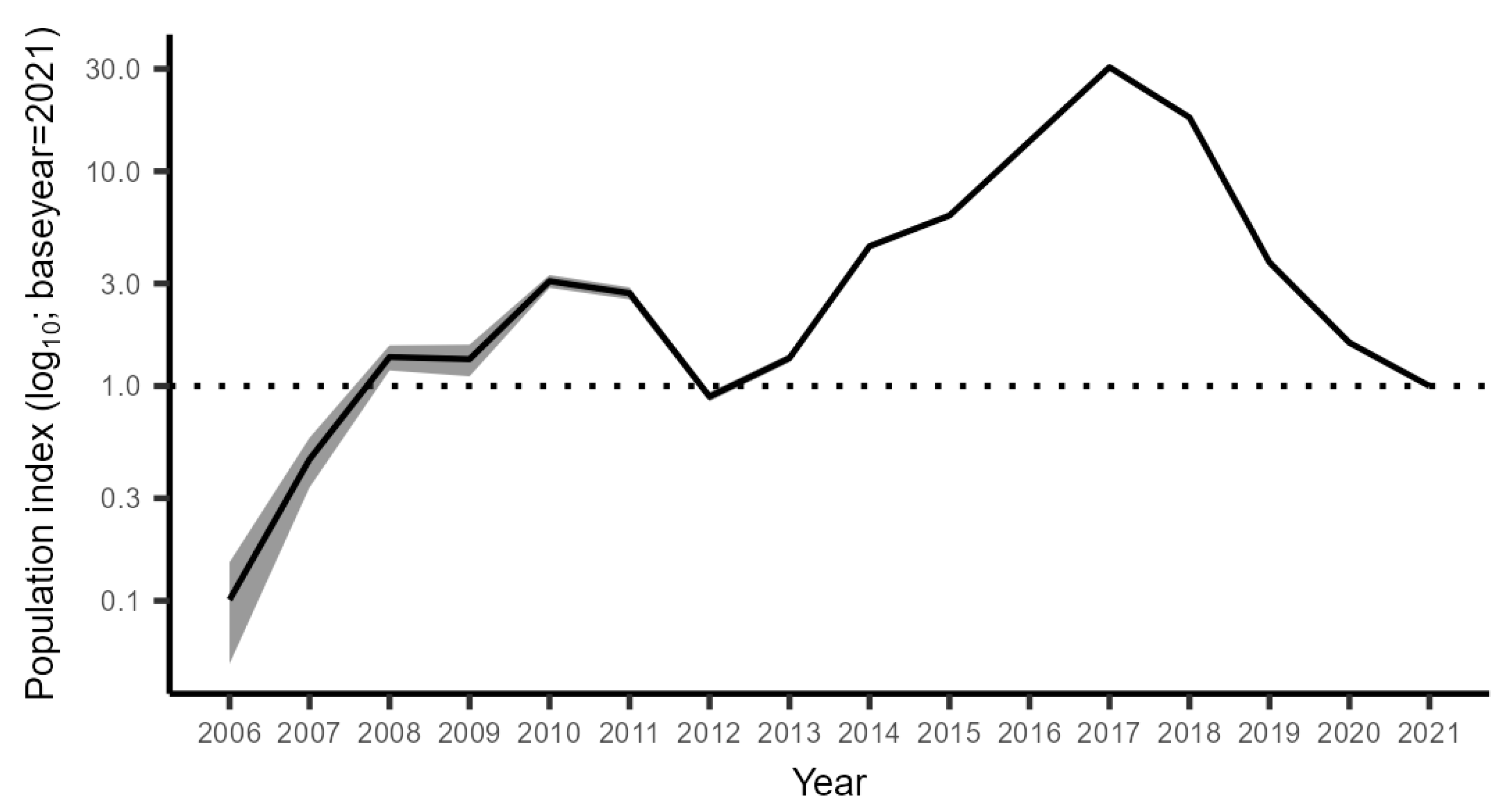
3.2.2. The Trend in the Gulf of Riga from GORDEM

The TRIM analysis of the GORDEM data suggests an overall strong increase in the RG population until 2017 (p < 0.0001, Figure 6), with an annual rate of change of 1.19 (±0.015 S.E.). Following this increase, over time, there was a rather dramatic decline in the estimated population index between 2018 and 2021. The population size in 2021 was about five times higher than that of 2012, while a comparable comparison for 2017 indicated a population size approximately 200 times greater than that of 2012.

3.2.3. The Trend in Open Sea from BITS

RG was first recorded in the open sea section of the Latvian EEZ in the BITS survey in 2010. Due to the assumptions of the TRIM method (see methods section), however, we could only perform a population change analysis using data from 2015 onward. This analysis suggests an overall strong decrease (p < 0.0001 Figure 7), with an annual rate of change of 0.63 (±0.049 S.E.) between 2015 and 2017. As for the GORDEM data, this trend was followed by a sharp decline during 2018–2021. The 2021 population index is similar to that of 2015.

3.2.4. Combined Trend across All Monitoring Data

By combining the population change indices from scientific monitoring (CFM, GORDEM, and BITS) data, we tested a combined TRIM model for RG in the Latvian EEZ. The results suggest a steep population increase until 2017, followed by a rapid decline (Figure 8). The strong increase (p < 0.0001) between 2006 and 2017 had an annual rate of change of 1.17 (±0.015 S.E.), and the estimated population size in 2021 was about 7.6 times higher than that of 2006, but 30 times smaller compared to that recorded in 2017.

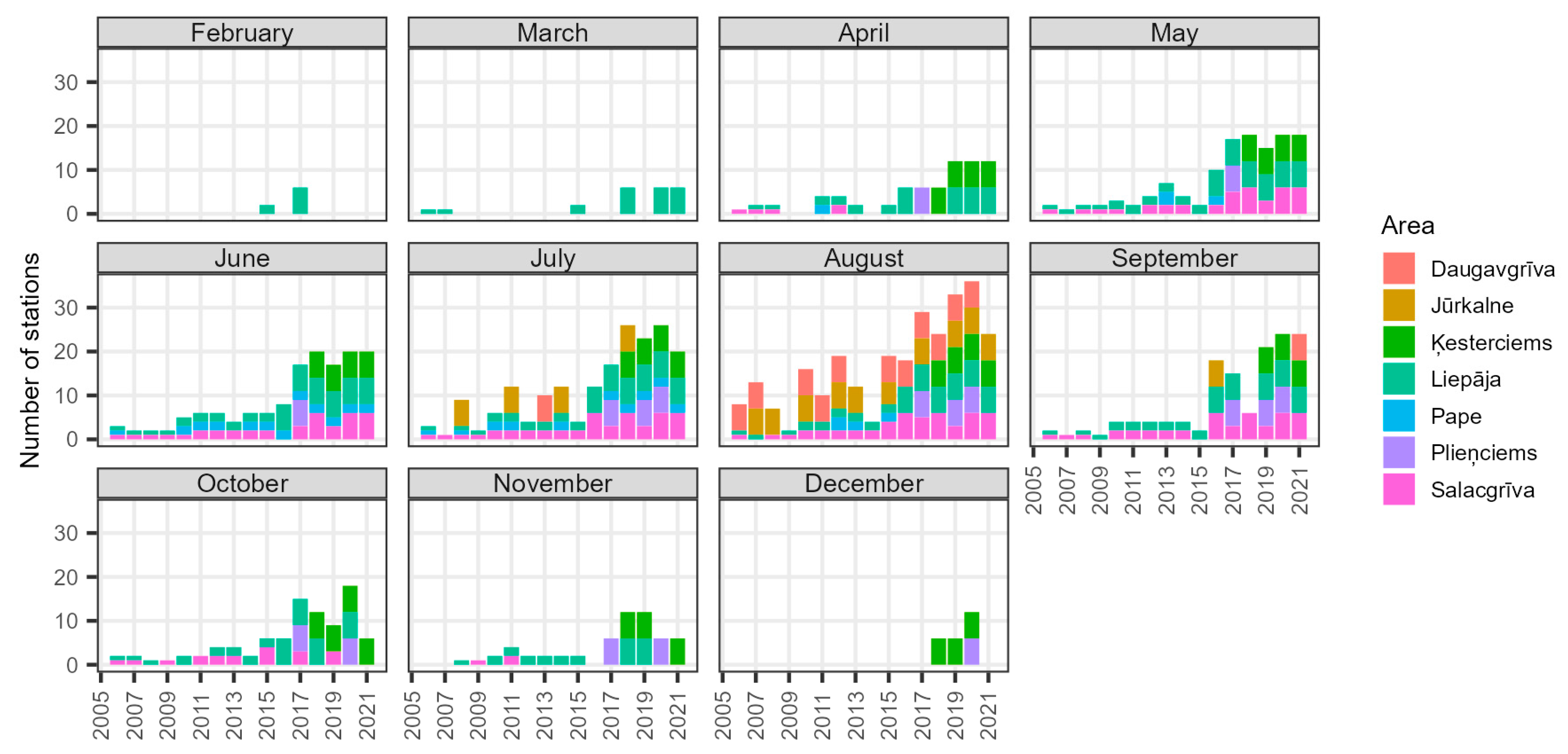
3.2.5. Monthly Catch Rates

To discover the period during the year in which it is most suitable to monitor RG population development, we extracted monthly catch rates from the CFM model (Figure 9). The highest catches occurred in May, being approximately 10 times higher than those recorded in late summer and autumn. The values in April and June were about half of the peak catches recorded in May. We, therefore, conclude that monitoring of RG in coastal areas should be focused on the time period between late April and early June, as the catches between years may vary to some extent.

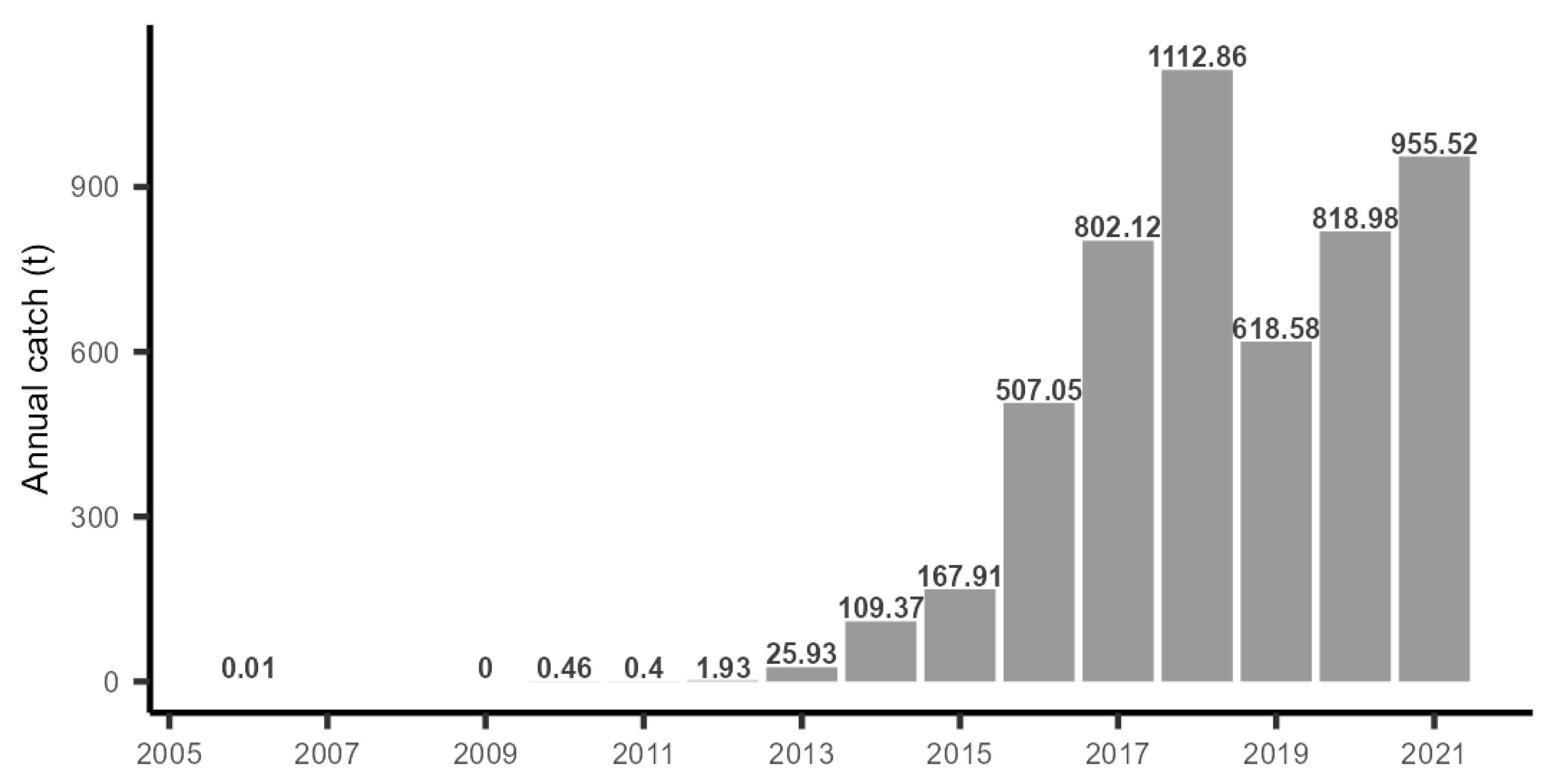
3.3. Catch Records in the Coastal Fishery

The first record of round goby near the Latvian coast was made in 2004 near Liepaja (the southwestern corner of the Latvian coast). However, the first commercial catches of RG on the Latvian coast appeared two years later, when the annual catches were only 6.3 kg. In the coming years, a sharp increase in the population size occurred, and logbook data from the fishery evidence an increase in RG catches. RG catches increased from less than 1 ton in 2011 to over 1112 tons in 2018, recording a slight decrease after this year (Figure 10). Recently, commercial landing increased in the eastern part of the Gulf of Riga (Figure A3), while the total landings suggest a recent decline in RG prevalence (Figure 10).

4. Discussion

There are several challenges in studying the temporal population development of wildlife species when using different in gears or monitoring methods. In this study, we merged all available long-term RG monitoring data in Latvia and found the applicability of an innovative approach to characterize fish population development using a method that is yet widely used in ornithological studies: the TRIM tool. This approach is widely used in by the European Bird Census Council when calculating Europe-wide species population trends [41]. We are not aware of any fisheries-related cases in the application of this method. Nevertheless, we consider that in processing any kind of animal taxon monitoring data, a well-adapted statistical analysis method should function effectively.

We could perform method combination by, firstly, inter-calibrating historical data sets to be comparable with the present methodology. We, therefore, developed applicable recalculation coefficients to be used in further studies. Secondly, we modeled and combined RG population trends obtained from different monitoring methods, finding a potential tipping point of the RG invasion in 2017, as also evidenced by commercial fishery landing records. Finally, we provided suggestions for improved planning of monitoring methods by accounting for seasonal differences in the catchability of RG.

4.1. Intercalibration

To the best of our knowledge, earlier comparisons between multi-mesh gillnets and other sampling methods and designs did not focus on intercalibration using conversion coefficients across gears [44,45]. Our study is, therefore, the first to do so and specifically focus on RG. We suggest that our results can be applied to data in other regions to improve the knowledge of RG population development. However, small fish species and juveniles are usually not representatively sampled by the gears used [29,31], and a combination of methods (active and passive fishing gears) should be used to cover the whole size-spectrum of the targeted fish community. We still believe that our study is relevant, despite the fact that we do not have reliable data on small fish.

When comparing models accounting for different random effects structures, the best model only included the factor “area”, with only marginal effects on explained variation (the difference between the conditional and marginal pseudo-determination coefficients). In terms of pseudo-determination coefficients, a similar fit to our best model was also found in the models considering the factors “station” and “station-in-area”; however, their performance, given their complexity, was lower (higher AICc values). This finding suggests that some site-specific effects on catchability or gear preference exist, though they may be a result of random factors related to fish movement. Our results further highlight that more general (wider-scale) aspects of the environment have some influence on the catchability of RG across gears. This result could possibly be related to differences in water visibility across sampling sites and variations in hydrological factors, since coastal monitoring is performed in seven different sites covering all seasonal quarters of the year over multiple years. This issue, in turn, may affect the catchability, as the gear is made of different linen (see Section 2.2.1). Moreover, monitoring sites are different in terms of substrate and water quality, being located in different conditions related to river estuaries of different sizes. Even though some monitoring areas provide more data (imbalanced data), the use of random effects modeling provides a generalization of the population trends [46]. However, the generalization is limited to the gear itself if “Nordic nets” are more like standard nets and “Coastal nets” are made of different linen. We suggest the use of the recalculation coefficients obtained in this study only in the case of comparable gear (see Section 2.2.1 on gear description for more details).

4.2. Population Development

As a result of the data used, the approach applied in this study did not address the change in the total abundance of RG in Latvian waters. Instead, we addressed trends in relative abundance. The data suggest an increase in relative abundance until 2017, whereafter the population drastically decreases. One probable cause of this is high fishing pressure [4], though a decline in 2018 is also observed in other coastal areas in the Baltic Sea (J. Olsson, personal comment). Overall, the results are reliable because we see similar trends across all three monitoring methods. The results are also supported by trends in commercial fisheries landings; however, the trends in landings data can be influenced by several factors besides population abundance, such as fishing pressure, market demand, and misreporting [47,48]. Nevertheless, considering the strong RG population increase in Latvian waters following its invasion and the large amount of registered commercial catches of the species, both data types support each other’s conclusions.

As we observed near-functional correlations between standardized and round-to-integer counts, we expect no influence on the population trends because of the rounding error. All methods-specific models agree on a large peak in population density in 2017, which was followed by a strong decline. This decline is of particular interest, but cannot be related to some difference in the sampling design, as monitoring schemes did not change and the data analysis method was based on site-at-time relationships.

There could be multiple factors affecting the results achieved in this study, such as hydrological anomalies at the bottom layer of the sampling site, an increase in targeted fishing, and local predators’ adaption during the study years.

Despite overall climate change and possible regime shift in ecosystem functioning in the Gulf of Riga [49], no major hydrological abnormalities were observed in the Latvian part of the Baltic Sea within the study period (BIOR unpublished hydrographical data until 2021) [50]. The high thermal resilience of the RG [8], as well as the stable oxygen levels at the main distribution area of the RG [51], indicate a low possibility of abiotic influence on the population trends. The yearly increase in targeted fishing for RG arguably affected the overall population development. Besides fishing mortality, other pressures, such as natural predation, could affect RG population development as the local ecosystems might respond to the presence of a new species. There is evidence that local predatory fish could successfully adopt their feeding strategies towards new invasive species [16,18,52], hence suppressing further population expansion.

It is, however, unclear how fishing and predation directly interact with RG population changes in Latvian waters; thus, this should be an object for future studies.

4.3. Suggestions for Future Monitoring Programs on RG

To the best of our knowledge, there is, to date, no comprehensive monitoring program for RG in the Baltic Sea. Coastal Fish monitoring is conducted with slight differences in the methodology in different countries [30]. This monitoring strategy is not suitable for RG, hence limiting the potential for regional comparisons of RG population trends. As the species is today widespread in the Baltic Sea, it might have negative effects on local ecosystems; thus, in some areas that are important for small-scale fisheries, we think that a regional monitoring program is needed.

Following the results of this study, we suggest that the best period to monitor RG is during the spring spawning migration, when the species is active, occurs in high numbers, and specimens are, thus, easier to catch. Our results also show more activity in shallow coastal waters compared to more offshore and deeper waters. “Nordic nets” seem to be the best gear since they are widely used across the Baltic Sea [30], and are suitable to cover a wide range of bottom types and marine biotopes in all depth zones of the coastal area in the Baltic Sea. Moreover, this method allows us to sample a wider size range of the RG than the standard “Coastal nets” (see Figure 2) In all, we suggest monitoring round goby in coastal areas during the spring using “Nordic nets”.

5. Conclusions

The highest commercial landings of RG are observed in the central Baltic Sea, of which 85% are caught in Latvian coastal waters [53]. In this study, we conclude that the significant increase in RG landings in the coastal fisheries of Latvia during the 2010s is likely attributed to a population increase and a more targeted fishery. As an invasive species, the current management goal for RG in Latvia is not to ensure the long-term sustainability of the stock, but to reduce the impact of this species on the native marine life as much as possible [53]. We assume that, after 2016, the Latvian fishing industry achieved the necessary knowledge for the effective acquisition of the RG as a target species and resource. RG is of high economic importance to fishers in Latvia, and for a more reliable assessment of the biomass of the species and to establish management targets, a stock-assessment model should be developed for the species.

References

1. Sapota, M.R. The Round Goby (Neogobius melanostomus) in the Gulf of Gdańsk—A Species Introduction into the Baltic Sea. Hydrobiologia 2004, 514, 219–224. [Google Scholar] [CrossRef]
2. Kuczyński, J. Babka krągła N. melanostomus (Pallas, 1811)—Emigrant z Basenu Pontokaspijskiego w Zatoce Gdańskiej. Bull. Sea Fish. Inst. 1995, 135, 68–71. [Google Scholar]
3. Sciences, A. Abundance and Distribution of Round Goby. Available online: https://helcom.fi/wp-content/uploads/2020/06/BSEFS-Abundance-and-distribution-of-round-goby.pdf (accessed on 18 May 2023).
4. ICES. Ices Scientific Reports Rapports Scientifiques Du Ciem Ices Workshop on Stickleback and Round Goby in the Baltic Sea (Wkstargate); ICES: Copenhagen, Denmark, 2022. [Google Scholar] [CrossRef]
5. Ojaveer, E. Ecosystems and Living Resources of the Baltic Sea; Springer: Cham, Switzerland, 2017; ISBN 9783319530093. [Google Scholar]
6. Holmes, M.; Kotta, J.; Persson, A.; Sahlin, U. Marine Protected Areas Modulate Habitat Suitability of the Invasive Round Goby (Neogobius melanostomus) in the Baltic Sea. Estuar. Coast. Shelf Sci. 2019, 229, 106380. [Google Scholar] [CrossRef]
7. Saraiva, S.; Markus Meier, H.E.; Andersson, H.; Höglund, A.; Dieterich, C.; Gröger, M.; Hordoir, R.; Eilola, K. Uncertainties in Projections of the Baltic Sea Ecosystem Driven by an Ensemble of Global Climate Models. Front. Earth Sci. 2019, 6, 244. [Google Scholar] [CrossRef]
8. Christensen, E.A.F.; Norin, T.; Tabak, I.; Van Deurs, M.; Behrens, J.W. Effects of Temperature on Physiological Performance and Behavioral Thermoregulation in an Invasive Fish, the Round Goby. J. Exp. Biol. 2021, 224, jeb237669. [Google Scholar] [CrossRef] [PubMed]
9. Reid, H.B.; Ricciardi, A. Ecological Responses to Elevated Water Temperatures across Invasive Populations of the Round Goby (Neogobius melanostomus) in the Great Lakes Basin. Can. J. Fish. Aquat. Sci. 2022, 79, 277–288. [Google Scholar] [CrossRef]
10. Kornis, M.S.; Mercado-Silva, N.; vander Zanden, M.J. Twenty Years of Invasion: A Review of Round Goby Neogobius melanostomus Biology, Spread and Ecological Implications. J. Fish Biol. 2012, 80, 235–285. [Google Scholar] [CrossRef]
11. Kotta, J.; Nurkse, K.; Puntila, R.; Ojaveer, H. Shipping and Natural Environmental Conditions Determine the Distribution of the Invasive Non-Indigenous Round Goby Neogobius melanostomus in a Regional Sea. Estuar. Coast. Shelf Sci. 2016, 169, 15–24. [Google Scholar] [CrossRef]
12. Azour, F.; van Deurs, M.; Behrens, J.; Carl, H.; Hüssy, K.; Greisen, K.; Ebert, R.; Møller, P.R. Invasion Rate and Population Characteristics of the Round Goby Neogobius melanostomus: Effects of Density and Invasion History. Aquat. Biol. 2015, 24, 41–52. [Google Scholar] [CrossRef] [Green Version]
13. Ustups, D.; Bergström, U.; Florin, A.B.; Kruze, E.; Zilniece, D.; Elferts, D.; Knospina, E.; Uzars, D. Diet Overlap between Juvenile Flatfish and the Invasive Round Goby in the Central Baltic Sea. J. Sea Res. 2016, 107, 121–129. [Google Scholar] [CrossRef]
14. Nurkse, K.; Kotta, J.; Orav-Kotta, H.; Ojaveer, H. A Successful Non-Native Predator, Round Goby, in the Baltic Sea: Generalist Feeding Strategy, Diverse Diet and High Prey Consumption. Hydrobiologia 2016, 777, 271–281. [Google Scholar] [CrossRef]
15. Matern, S.; Herrmann, J.P.; Temming, A. Differences in Diet Compositions and Feeding Strategies of Invasive Round Goby Neogobius melanostomus and Native Black Goby Gobius Niger in the Western Baltic Sea. Aquat. Invasions 2021, 16, 314–328. [Google Scholar] [CrossRef]
16. Almqvist, G.; Strandmark, A.K.; Appelberg, M. Has the Invasive Round Goby Caused New Links in Baltic Food Webs? Environ. Biol. Fishes 2010, 89, 79–93. [Google Scholar] [CrossRef]
17. Crane, D.P.; Farrell, J.M.; Einhouse, D.W.; Lantry, J.R.; Markham, J.L. Trends in Body Condition of Native Piscivores Following Invasion of Lakes Erie and Ontario by the Round Goby. Freshw. Biol. 2015, 60, 111–124. [Google Scholar] [CrossRef]
18. Hempel, M.; Neukamm, R.; Thiel, R. Effects of Introduced Round Goby (Neogobius melanostomus) on Diet Composition and Growth of Zander (Sander lucioperca), a Main Predator in European Brackish Waters. Aquat. Invasions 2016, 11, 167–178. [Google Scholar] [CrossRef]
19. Oesterwind, D.; Bock, C.; Förster, A.; Gabel, M.; Henseler, C.; Kotterba, P.; Menge, M.; Myts, D.; Winkler, H.M. Predator and Prey: The Role of the Round Goby Neogobius melanostomus in the Western Baltic. Mar. Biol. Res. 2017, 13, 188–197. [Google Scholar] [CrossRef] [Green Version]
20. Rakauskas, V.; Putys, Ž.; Dainys, J.; Lesutiene, J.; Ložys, L.; Arbačiauskas, K. Increasing Population of the Invader Round Goby, Neogobius melanostomus (Actinopterygii: Perciformes: Gobiidae), and Its Trophic Role in the Curonian Lagoon, SE Baltic Sea. Acta Ichthyol. Piscat. 2013, 43, 95–108. [Google Scholar] [CrossRef] [Green Version]
21. Jakubas, D. The Response of the Grey Heron to a Rapid Increase of the Round Goby. Waterbirds 2004, 27, 304–307. [Google Scholar] [CrossRef]
22. Behrens, J.W.; Ryberg, M.P.; Einberg, H.; Eschbaum, R.; Florin, A.B.; Grygiel, W.; Herrmann, J.P.; Huwer, B.; Hüssy, K.; Knospina, E.; et al. Seasonal Depth Distribution and Thermal Experience of the Non-Indigenous Round Goby Neogobius melanostomus in the Baltic Sea: Implications to Key Trophic Relations. Biol. Invasions 2022, 24, 527–541. [Google Scholar] [CrossRef]
23. Karlson, A.M.L.; Almqvist, G.; Skóra, K.E.; Appelberg, M. Indications of Competition between Non-Indigenous Round Goby and Native Flounder in the Baltic Sea. ICES J. Mar. Sci. 2007, 64, 479–486. [Google Scholar] [CrossRef] [Green Version]
24. Järv, L.; Kotta, J.; Kotta, I.; Raid, T. Linking the Structure of Benthic Invertebrate Communities and the Diet of Native and Invasive Fish Species in a Brackish Water Ecosystem. Ann. Zool. Fennici 2011, 48, 129–141. [Google Scholar] [CrossRef]
25. Funk, S.; Frelat, R.; Möllmann, C.; Temming, A.; Krumme, U. The Forgotten Feeding Ground: Patterns in Seasonal and Depth-Specific Food Intake of Adult Cod Gadus Morhua in the Western Baltic Sea. J. Fish Biol. 2021, 98, 707–722. [Google Scholar] [CrossRef] [PubMed]
26. Bowser, J.; Galarowicz, T.; Murry, B.; Johnson, J. Invasive Species Appearance and Climate Change Correspond with Dramatic Regime Shift in Thermal Guild Composition of Lake Huron Beach Fish Assemblages. Fishes 2022, 7, 263. [Google Scholar] [CrossRef]
27. Liversage, K.; Nurkse, K.; Kotta, J.; Järv, L. Environmental Heterogeneity Associated with European Perch (Perca fluviatilis) Predation on Invasive Round Goby (Neogobius melanostomus). Mar. Environ. Res. 2017, 132, 132–139. [Google Scholar] [CrossRef] [PubMed]
28. Pannekoek, J.; Van Strien, A. TRIM 3 Manual (TRends & Indices for Monitoring Data); Statistics Netherlands: Hague, The Netherlands, 2005; pp. 1–58. [Google Scholar]
29. Bernes, C. Change Beneath the Surface: An In-Depth Look at Sweden’s Marine Environment; Royal Swedish Academy of Sciences: Stockholm, Sweden, 2005; ISBN 9162012460, 9789162012465. [Google Scholar]
30. Neuman, E.; Sandstrom, O.G.T. Guidelines for Coastal Fish Monitoring. Natl. Board Fish. Inst. Coast. Reserch 1997, 44, 1–19. [Google Scholar]
31. ICES Manual for the Baltic International Trawl Surveys (BITS) Version 2.0; ICES: Copenhagen, Denmark, 2017; ISBN 9788774821533.
32. Olsson, J.; Bergström, L.; Gårdmark, A. Abiotic Drivers of Coastal Fish Community Change during Four Decades in the Baltic Sea-ICES. J. Mar. Sci. 2012, 69, 961–970. [Google Scholar] [CrossRef]
33. Wood, S.N. Generalized Additive Models: An Introduction with R; Chapman and Hall/CRC: Boca Raton, FL, USA, 2006. [Google Scholar]
34. Burnham, K.P.; Anderson, D.R. Model Selection and Multimodel Inference: A Practical Information-Theoretic Approach, 2nd ed.; Springer: New York, NY, USA, 2002; ISBN 0387953647. [Google Scholar]
35. R Core Team. R: A Language and Environment for Statistical Computing; R Core Team: Vienna, Austria, 2022. [Google Scholar]
36. Wood, S.; Scheipl, F. Gamm4: Generalized Additive Mixed Models Using “mgcv” and “Lme4”. 2020. Available online: https://cran.r-project.org/web/packages/gamm4/gamm4.pdf (accessed on 10 February 2023).
37. Wood, S.N. Fast Stable Restricted Maximum Likelihood and Marginal Likelihood Estimation of Semiparametric Generalized Linear Models. J. R. Stat. Soc. 2011, 73, 3–36. [Google Scholar] [CrossRef] [Green Version]
38. Wickham, H.; Averick, M.; Bryan, J.; Chang, W.; McGowan, L.; François, R.; Grolemund, G.; Hayes, A.; Henry, L.; Hester, J.; et al. Welcome to the Tidyverse. J. Open Source Softw. 2019, 4, 1686. [Google Scholar] [CrossRef] [Green Version]
39. Sokal, R.R.; Rohlf, F.J.J. Biometry: The Principles and Practice of Statistics in Biological Research, 3rd ed.; W.H. Freeman and Company: New York, NY, USA, 1995; ISBN 9780716724117. [Google Scholar]
40. Pannekoek, J.; Bogaart, P.; van der Loo, M. Models and Statistical Methods in Rtrim; CBS Discussion Paper; Statistics Netherlands: Hague, The Netherlands, 2018; pp. 1–34. [Google Scholar]
41. Van Strien, A.J.; Pannekoek, J.; Gibbons, D.W. Indexing European Bird Population Trends Using Results of National Monitoring Schemes: A Trial of a New Method. Bird Study 2001, 48, 200–213. [Google Scholar] [CrossRef]
42. Bogaart, P.; van der Loo, M.; Pannekoek, J. Rtrim: Trends and Indices for Monitoring Data; Statistics Netherlands: Voorburg, The Netherlands, 2020. [Google Scholar]
43. Urban-Malinga, B.; Wodzinowski, T.; Witalis, B.; Zalewski, M.; Radtke, K.; Grygiel, W. Marine Litter on the Seafloor of the Southern Baltic. Mar. Pollut. Bull. 2018, 127, 612–617. [Google Scholar] [CrossRef]
44. Rotherham, D.; Gray, C.A.; Broadhurst, M.K.; Johnson, D.D.; Barnes, L.M.; Jones, M.V. Sampling Estuarine Fish Using Multi-Mesh Gill Nets: Effects of Panel Length and Soak and Setting Times. J. Exp. Mar. Bio. Ecol. 2006, 331, 226–239. [Google Scholar] [CrossRef]
45. Specziár, A.; Eros, T.; György, Á.I.; Tátrai, I.; Bíró, P. A Comparison between the Benthic Nordic Gillnet and Whole Water Column Gillnet for Characterizing Fish Assemblages in the Shallow Lake Balaton. Ann. Limnol. 2009, 45, 171–180. [Google Scholar] [CrossRef]
46. Zuur, A.F.; Ieno, E.N.; Walker, N.J.; Saveliev, A.A.; Smith, G.M. Mixed Effects Models and Extensions in Ecology with R; Springer: New York, NY, USA, 2009; ISBN 9780387874579. [Google Scholar]
47. Olsson, J.; Andersson, M.L.; Bergström, U.; Arlinghaus, R.; Audzijonyte, A.; Berg, S.; Briekmane, L.; Dainys, J.; Ravn, H.D.; Droll, J.; et al. A Pan-Baltic Assessment of Temporal Trends in Coastal Pike Populations. Fish. Res. 2023, 260, 106594. [Google Scholar] [CrossRef]
48. Lappalainen, A.; Hyvönen, J.; Söderkultalahti, P.; Heikkinen, J. Estimating Annual Cpue Indices for Perch (Perca fluviatilis) from Monthly Logbook Data of a Gill-Net Fishery in the Bothnian Bay, Baltic Sea. Boreal Environ. Res. 2020, 25, 79–91. [Google Scholar]
49. Kortsch, S.; Frelat, R.; Pecuchet, L.; Olivier, P.; Putnis, I.; Bonsdorff, E.; Ojaveer, H.; Jurgensone, I.; Strāķe, S.; Rubene, G.; et al. Disentangling Temporal Food Web Dynamics Facilitates Understanding of Ecosystem Functioning. J. Anim. Ecol. 2021, 90, 1205–1216. [Google Scholar] [CrossRef] [PubMed]
50. Andersson, L. Hydrography and Oxygen in the Deep Basins. HELCOM Balt. Sea Environ. Fact Sheets. 2014, Volume 1–6. Available online: https://helcom.fi/wp-content/uploads/2019/08/BSEFS_Hydrography-and-oxygen-in-the-deep-basins_2010.pdf (accessed on 18 May 2023).
51. Casini, M.; Hansson, M.; Orio, A.; Limburg, K. Changes in Population Depth Distribution and Oxygen Stratification Are Involved in the Current Low Condition of the Eastern Baltic Sea Cod (Gadus morhua). Biogeosciences 2021, 18, 1321–1331. [Google Scholar] [CrossRef]
52. Tiralongo, F.; Messina, G.; Lombardo, B.M. Invasive Species Control: Predation on the Alien Crab Percnon gibbesi (H. Milne Edwards, 1853) (Malacostraca: Percnidae) by the Rock Goby, Gobius paganellus Linnaeus, 1758 (Actinopterygii: Gobiidae). J. Mar. Sci. Eng. 2021, 9, 393. [Google Scholar] [CrossRef]
53. Ustups, D. Latvian Fisheries Yearbook; The Latvian Rural Advisory and Training Centre: Ozolnieku pagasts, Latvia, 2021; Volume 25. [Google Scholar]
Figure 1. Study area: (a) Latvia (dark grey) in Baltic Sea (in blue) in Europe; (b) Latvian exclusive economic zone (light grey) and monitoring sites (red dots—coastal areas, crosses—Gulf of Riga, X—open sea).
Fishes 08 00305 g001
Figure 2. Description of gear calibration data: (a) number of calibration surveys in years over seasonal quarters, and (b) total number of individuals per length group (cm) captured for two monitoring gears.
Fishes 08 00305 g002
Figure 3. Temporal distribution of number of stations per area in coastal fish monitoring.
Fishes 08 00305 g003
Figure 4. Population level proportion of individuals per length group expected to be captured in “Coastal nets” assuming that they are caught simultaneously with “Nordic nets”. Dotted vertical lines represent weighted mean lengths of individuals smaller than 10 cm or larger than 21 cm.
Fishes 08 00305 g004
Figure 5. Population changes (yearly indices with standard error) of round goby at coastal monitoring sites. Y-axis represents population size relative to population in 2021 on a logarithmic scale. The dotted line represents the relative population size at the base year (2021).
Fishes 08 00305 g005
Figure 6. Population changes (yearly indices with standard error) of round goby in Gulf of Riga. Y-axis represents population size relative to population in 2021 on a logarithmic scale. The dotted line represents the relative population size at the base year (2021).
Fishes 08 00305 g006
Figure 7. Population changes (yearly indices with standard error) of round goby in open sea. Y-axis represents population size relative to population in 2021 on a logarithmic scale. The dotted line represents the relative population size at the base year (2021).
Fishes 08 00305 g007
Figure 8. Population changes (yearly indices with standard error) of round goby in Latvian exclusive economic zone in Baltic Sea. Y-axis represents population size relative to population in 2021 on a logarithmic scale. The dotted line represents the relative population size at the base year (2021).
Fishes 08 00305 g008
Figure 9. Multiplicative coefficients (base is February) of RGs catchability in coastal fisheries monitoring program during years 2006–2021. For each month, average relative catches across years are plotted with a standard error bar (SE), the dotted line represents relative catchability at the base month (February).
Fishes 08 00305 g009
Figure 10. Annual catches of RG in Latvian coastal waters.
Fishes 08 00305 g010