Article

Use of Ensemble Model for Modeling the Larval Fish Habitats of Different Ecological Guilds in the Yangtze Estuary

1
Fisheries College, Ocean University of China, Qingdao 266000, China
2
National Engineering Research Center for Oceanic Fisheries, Key Laboratory of Sustainable Exploitation of Oceanic Fisheries Resources (Ministry of Education), College of Marine Sciences, Shanghai Ocean University, Shanghai 201306, China
3
Key Laboratory of Marine Ecological Monitoring and Restoration Technologies, Shanghai 201306, China
4
Joint Laboratory for Monitoring and Conservation of Aquatic Living Resources in the Yangtze Estuary, Shanghai 201306, China
5
Scientific Observing and Experimental Station of Fishery Resources for Key Fishing Grounds, Ministry of Agriculture, Key Laboratory of Sustainable Utilization of Technology Research for Fisheries Resources of Zhejiang Province, Marine Fisheries Research Institute of Zhejiang, Zhoushan 316000, China
*
Author to whom correspondence should be addressed.
Fishes 2023, 8(4), 209; https://doi.org/10.3390/fishes8040209
Submission received: 17 March 2023 / Revised: 13 April 2023 / Accepted: 14 April 2023 / Published: 17 April 2023
(This article belongs to the Special Issue Fisheries and Aquaculture Engineering)

Abstract

:
Estuaries provide nursery habitats for a variety of fish species of different ecological guilds and have complicated environmental conditions. In this study, we applied ensemble species distribution models (SDMs) to four abundant and different ecological guild larval fish species (Hemiculter bleekeri (freshwater guild), Pseudolaubuca sinensis (freshwater guild), Coilia mystus (brackish water guild), and Engraulis japonicus (marine guild)) to explore their suitable habitats and the fish–habitat relationships in the Yangtze Estuary. The results showed that random forest (RF) demonstrated the best performance in all single algorithms and the surface range envelop (SRE) model was scarcely accurate. The ensemble SDMs demonstrated a superior predictive ability compared with any single algorithm, with the true skill statistic (TSS) and the area under the receiver operating characteristic curve (AUC) scores being above 0.899 and 0.641, respectively. Binary presence–absence maps showed the different spatial distribution patterns of the four species. We primarily found the freshwater species (P. sinensis and H. bleekeri) present in the South Branch (west of 122° E), whereas we found the marine species (E. japonicus) anywhere except inside the South Branch (west of 121.8° E). The area for P. sinensis (1615.93 km2) was relatively larger than that for H. bleekeri (1136.87 km2). We predicted that the brackish water species (C. mystus) would most likely be present inside the North Branch (west of 122° E), Eastern Chongming, and outside the South Branch (east of 121.8° E). Salinity, as a key environmental variable, contributed to the spatial variability. A low salinity (sea surface salinity (SSS) < 3) was beneficial for P. sinensis and H. bleekeri but was not suitable for E. japonicus. The SSS suitable range for C. mystus was 5–10 and 12–20. Multiple ecological guild species dwelled in the confluence of salt and fresh water. Our results will play an important role in the design of specific conservation strategies for fishery resources in this area.
Key Contribution: Suitable habitats of different ecological guild larval fishes are considered on the nursery grounds of larval fish in Yangtze Estuary. SSS is a key variable that contributes to spatial variability of different ecological guild species, and the confluence of salt and fresh waters is a place where multiple ecological guild species coexist.

Graphical Abstract

1. Introduction

Compared with adults, larval fish are characterized by their weak swimming ability, and they display a high inherent vulnerability to environmental variation [1]. Estuaries are one of the most biologically productive and valuable ecosystems on Earth, yet they are regarded as the most threatened and degraded ecosystem, with numerous stressors such as pollution, hydro-morphological changes, and invasive species present [2,3,4]. For estuarine larval fish, they can either originate from within the estuary or from marine and freshwater, which is directly related to the recruitment of estuarine fishery resources [5]. Considering the ecological importance of larval fish in estuarine ecosystems, an understanding of the suitable habitats of different ecological guild species (DES) is urgently needed for the purpose of more effectively protecting estuarine fishery resources [6,7,8]. Therefore, to understand the structure and function of estuaries, we must better understand the early life-cycle stages of DES in the estuary area [9].
The spatio–temporal variability of larval fish distribution is mainly related to oceanographic features, especially in the temperate region [10,11,12]. Oceanographic features (e.g., salinity and temperature) can affect both the metabolism and growth at the individual level and the spatio–temporal distribution at the population level for the larval fish in the estuarine area [13,14,15]. The distribution of larval fish is deeply influenced by environmental variables, including depth, temperature, and salinity [16,17]. The estuarine DES are distributed in different areas according to the change of salinity and temperature affected by the runoff, wind, and tide [18,19]. For example, DES estuarine fishes have different temperature habitat preferences, thus reducing competition between the species feeding on similar types of prey [19]. Therefore, understanding of fish–habitat relationships for DES larval fishes is very important for their future resource prediction related to climate change [20,21,22].
The Yangtze River is the world’s third longest river with a length of 6397 km, and its estuary is the largest estuary in the western Pacific Ocean [23]. It serves as an important nursing ground for varieties of fish species [14]. More than 100 larval fish species have been found and identified, mainly belonging to freshwater, brackish water, and marine ecological guilds [24,25]. The sea surface salinity (SSS), sea surface temperature (SST), chlorophyll-a concentration, and total suspended particulate matter were the major affecting environmental conditions [25,26]. The peak abundance of the larval fish in the Yangtze Estuary appeared in the spring, and the high abundances were mainly due to the presence of several dominant species, including Hemiculter bleekeri (freshwater guild), Pseudolaubuca sinensis (freshwater guild), Coilia mystus (brackish water guild), and Engraulis japonicus (marine guild) [27,28]. All four species are small pelagic fishes with a strong reproductive and survival ability and are usually the prey of many other carnivorous fish, such as the threatened Chinese sturgeon (Acipenser sinensis) [29]. The population abundances of these small pelagic fishes were mainly dependent on their recruitment process as to affect the balance of the ecosystem in the Yangtze Estuary [27]. Their habitats are at risk of decline. In particular, the yield of C. mystus has sharply declined in the past 30 years [30]. Recently, many studies have focused on the fish–habitat relationships of different life-cycle stages, especially on the larval fish stage in the Yangtze Estuary [31,32,33]. Considering severe habitat loss and degradation in estuaries (e.g., C. mystus) [30], managers need to identify, prioritize, and protect essential habitats for estuarine fish species. Hence, a suitable method to improve the accurate and reliable predictions of DES distributions in Yangtze Estuary is needed.
Prediction models have been used to simulate fish–habitat relationships and potential species distributions for estuarine species [20]. Among these models, species distribution models (SDMs) have become an important tool to examine a multitude of ecological and conservation-related questions [34,35,36,37]. Most previous studies conducting SDMs have only used single algorithms for estuarine fish species [8,20,30]. The single algorithms range from the most conventional and frequently used (e.g., generalized linear models (GLM) and generalized additive models (GAM)) to new and sophisticated machine-learning methods (e.g., random forests (RF)), with the latter often showing considerable increases in the model predicting capacity [38,39]. However, estuaries’ persistent environmental fluctuations and dynamic nature added difficulties in studying DES distributions, and thus, building their SDMs was challenging [40]. If the input data change, the performance of each single model may become unstable [41,42]. Thus, to assess the predictive uncertainty and increase the predictive accuracy of SDMs, a measure of the ensemble forecasting of species distributions is useful [35]. Due to the particular and dynamic nature of estuarine ecosystems, it is necessary to fully consider the suitability of DES and their habitat models [40]. Franca and Cabral (2019) built SDMs for four adult fish species in nine estuaries from the Portuguese coast and found that predictions obtained with the ensemble approach were more accurate [40]. Recently, researchers have widely recognized and used a modeling platform (biomod2) based on R software since its publication [22,43]. However, there are only a few applications of the ensemble models in the estuary area, particularly for the larval fish distributions (but see Zhang et al., 2020 [31]).
In this study, we constructed the ensemble SDMs for the four DES larval fish species (i.e., H. bleekeri, P. sinensis, C. mystus, and E. japonicus) in the Yangtze Estuary. We compared the performance of the ensemble SDMs to single models (i.e., random forest) to model the larval fish habitats. We further explored the special distinction of larval fish habitats under the complex hydrological environments of the Yangtze Estuary and explained the fish–habitat relationships for these four species. We expect that the conclusions from this study will provide insights into the spatial patterns of DES and will reveal the key environmental variables causing these patterns. Predicting their suitable habitats will have important implications for the conservation of the fishery resources in the Yangtze Estuary. These predictions can also enhance our understanding of how larval fish use estuaries. The results may also be applicable to other estuary ecosystems.

2. Materials and Methods

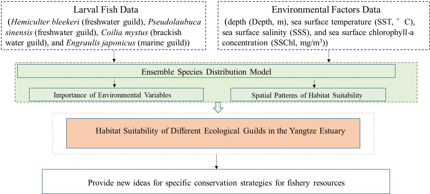
2.1. Study Area and Sampling

The Yangtze Estuary is the largest estuary in China, and it is located in the northwest East China Sea and southwest Yellow Sea. Chongming Island divides the estuary into the North and South Branches (Figure 1). The different areas of the Yangtze Estuary are geographically similar, but their hydrological conditions are different [30]. For example, the annual average salinity of the North Branch is about ten times greater than that of the South Branch [14]. We conducted three surveys in the sampling region (30.8° N–31.7° N, 121.3° E–122.5° E) based on a stratified random design in spring (May) from 2019 to 2021 (Figure 1). In total, we collected 168 larval fish samples (57 samples in 2019, 56 samples in 2020, and 55 samples in 2021) during daytime using a plankton net (0.505 mm mesh size, 80 cm in diameter, and 145 cm in length). We towed horizontally under the sea surface for 10 min at a constant speed of 2–3 knots (Table 1). We measured the depth, temperature, salinity, and chlorophyll-a concentration by using a Sea-bird 19 plus V2 CTD. We preserved all the samples in 5% formaldehyde in seawater for further identification in the laboratory. The larval fishes were identified by morphology observation under a microscope according to the study by Zhang et al. (1985) and Qiao (2005) [44,45]. In each sample, we noted whether each species was present or absent.

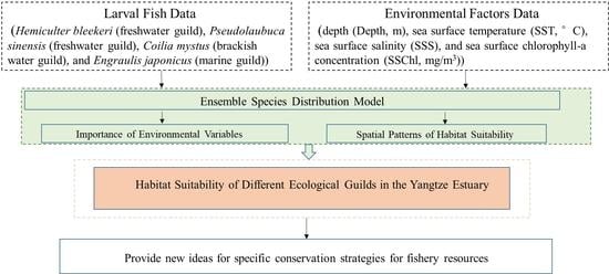
2.2. Environmental Variables

We selected four uncorrelated environmental variables for the subsequent modeling, including depth (Depth, m), sea surface temperature (SST, °C), sea surface salinity (SSS), and sea surface chlorophyll-a concentration (SSChl, mg/m3) (Table S1). To avoid over-fitting and multi-collinearity problems, we calculated the variance inflation factor (VIF) for each candidate predictor variable, and we removed the superfluous predictor variable (whose VIF value is higher than 2) in the preliminary study [46,47]. The diagnosis results showed that their collinearity was not significant (VIF < 2), so all four environmental factors were used for the subsequent study.

2.3. Ensemble Model Construction

Ensemble models can reduce the uncertainty caused by various algorithms in SDMs [48]. We used the biomod2 package to build an ensemble model. The package gathered some commonly used species distribution models, including classification methods (e.g., generalized boosting model and random forest) [39] and regression methods (e.g., generalized linear model and generalized additive model) [33]. For this study, we selected ten modeling algorithms, including artificial neural networks (ANN), classification tree analysis (CTA), flexible discriminant analysis (FDA), generalized additive model (GAM), generalized boosting model (GBM), generalized linear model (GLM), multiple adaptive regression splines (MARS), maximum entropy (MaxEnt), random forest (RF), and surface range envelop (SRE), to reveal the relationship between the four dominant species distribution data and the four environmental variables. To evaluate the performance of the different algorithms, we randomly divided the species distribution data into two parts, of which we used 70% of the data for model training and 30% of the data to evaluate the model prediction results. We repeated every modeling algorithm five times. We evaluated the performances of ten algorithms using the true skill statistic (TSS) and the area under the receiver operating characteristic curve (AUC) [49,50]. The AUC represents a model’s discriminative capacity with regard to the data and is obtained by plotting the commission error (1-specificity; false positives) on the horizontal axis versus the omission error (sensitivity; actual positives which are correctly identified as such) on the vertical axis for numerous thresholds. The AUC values range from 0 to 1 and the modeling algorithm shows a higher accuracy with a higher value. As an evaluation metric, the AUC has the advantage of being prevalence- and threshold independent [37]. The TSS is concerned with omission and commission errors and is also prevalence independent. The TSS ranges from −1 to +1, where +1 means perfect agreement and <0 means random performance [49]. We only selected algorithms with TSS > 0.4 and AUC > 0.7 to build the ensemble model [31]. We determined the relative importance of each environmental variable for the distributions of the four larval fishes with a randomization procedure where the principal idea is to shuffle a single variable of the given data [43]. The return score is 1−correlation between the reference’s predictions and the ’shuffled’ one. The higher the value, the more influence the variable has on the model. The projected habitat suitability values range from 0 to 1000, with 0 representing the lowest occurrence probability (i.e., 0) and 1000 representing the highest occurrence probability (i.e., 1). For each species, we converted the projected habitat suitability values into binary presence–absence maps by selecting a probability threshold that maximized the TSS value [37,43].
We conducted all analyses with R 64-bit (version 4.0.2, 64 bit) software (https://www.r-project.org, accessed on 22 July 2020), using the package “biomod2” for ensemble model construction [43], “raster” for data manipulation [51], “terra” for habitat area calculation [52], and “maps” and “ggplot2” for maps and figures, respectively [53,54].

3. Results

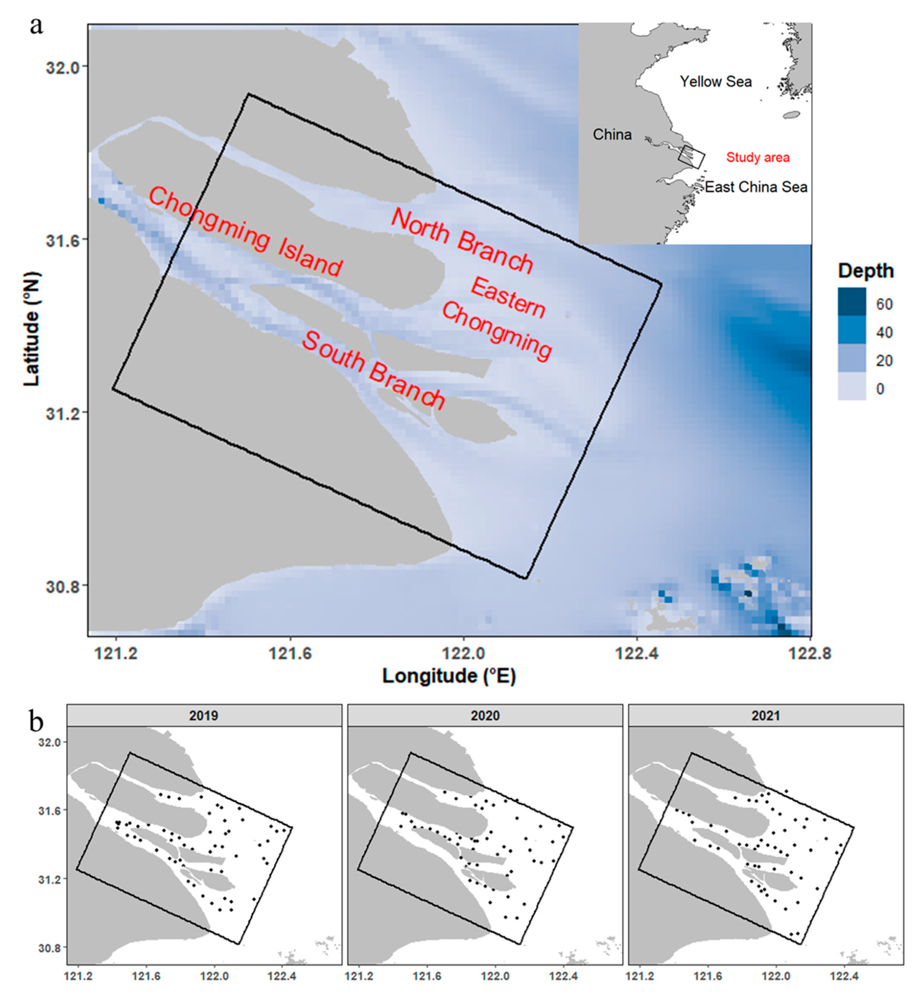
3.1. Model Accuracy Measures

The SDMs of E. japonicus performed worse than the other three species for every algorithm (Figure 2). Among the ten algorithms, the RF algorithm showed the best predictive abilities for all four larval fish, and the SRE algorithms were scarcely accurate. The algorithm performances of both GAM and GBM were also generally satisfactory with regard to the statistics, except when used with E. japonicus. The TSS and AUC scores of the ensemble models for the four species were above 0.899 and 0.641, respectively (Table 2). Additionally, the ensemble model exhibited a high specificity and sensitivity, with values above 78% (Table 2). Compared with any of the single modeling algorithms, the ensemble model had a more accurate performance. These results show that the predictive abilities of the ensemble model can reduce the uncertainty and increase the accuracy compared with the single model.

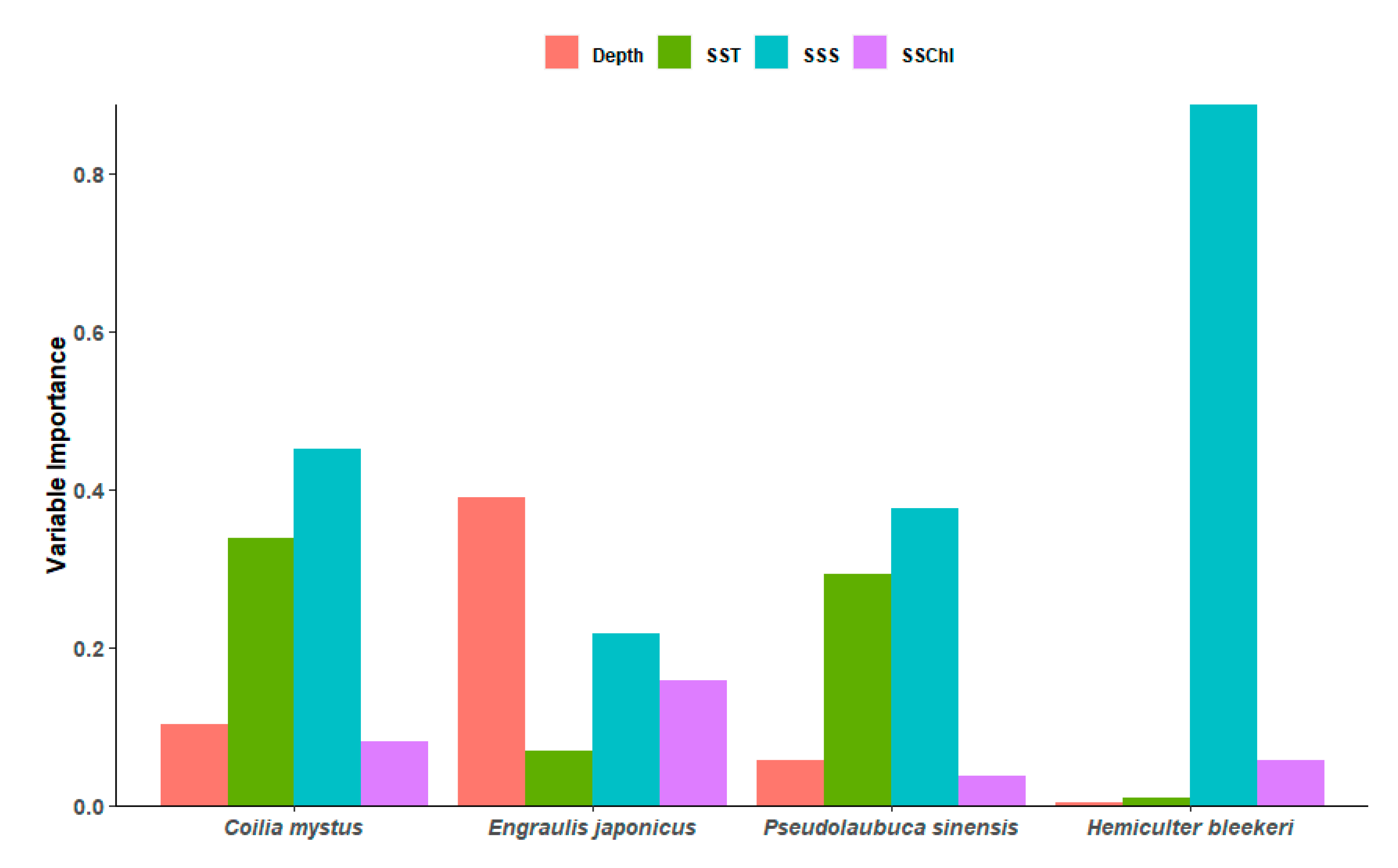
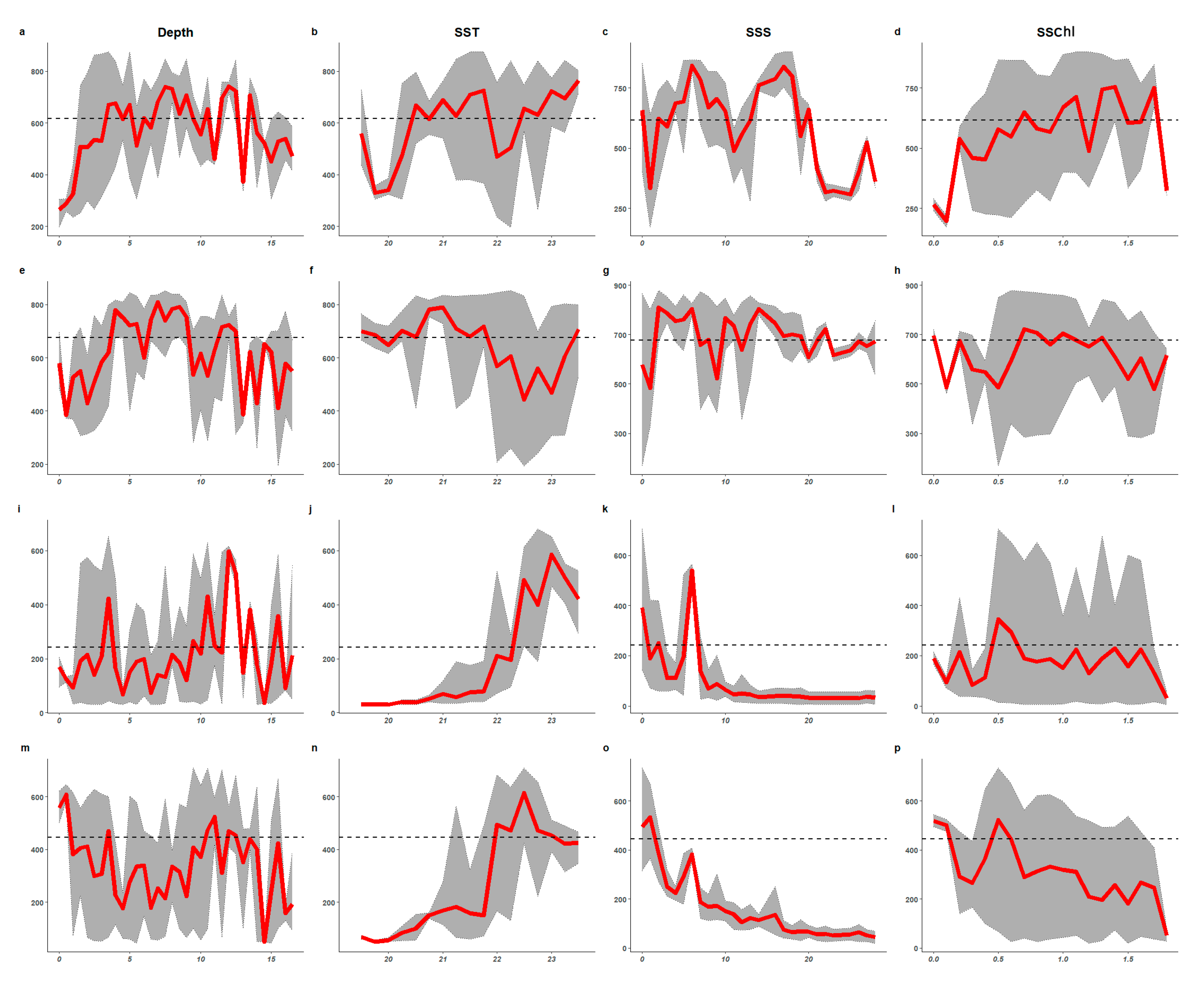
3.2. Importance of Environmental Variables and Response Curves

For all species except E. japonicus, the SSS was the most important variable in the ensemble model (Figure 3). The SSS (0.45) and SST (0.34) were the key influential variables to predict the occurrence probability of C. mystus. Depth (0.10) and SSChl (0.08) played a less pivotal role. Depth was the most important variable with a 0.39 importance value for E. japonicus. For P. sinensis, SST (0.29) also had a higher impact on the model performance. Apart from the strong influence of the SSS (0.83), the occurrence probability of H. bleekeri was scarcely influenced by the other three variables.
The shapes of the response curves of the different species were quite different (Figure 4). The SSS suitable ranges of C. mystus were 5–10 and 12–20. Low salinity (SSS < 3) was unsuitable for E. japonicus, but it was suitable for P. sinensis and H. bleekeri. The SST suitable ranges for C. mystus were 20.5–21.8 °C and higher than 22.5 °C. A high temperature range (SST higher than 22.3 °C) was ideal for P. sinensis and H. bleekeri, but it was unsuitable for E. japonicus. The most important variable that influenced the distribution of E. japonicus was depth, whereby a depth of 4 to 8 m maximized the occurrence probability.

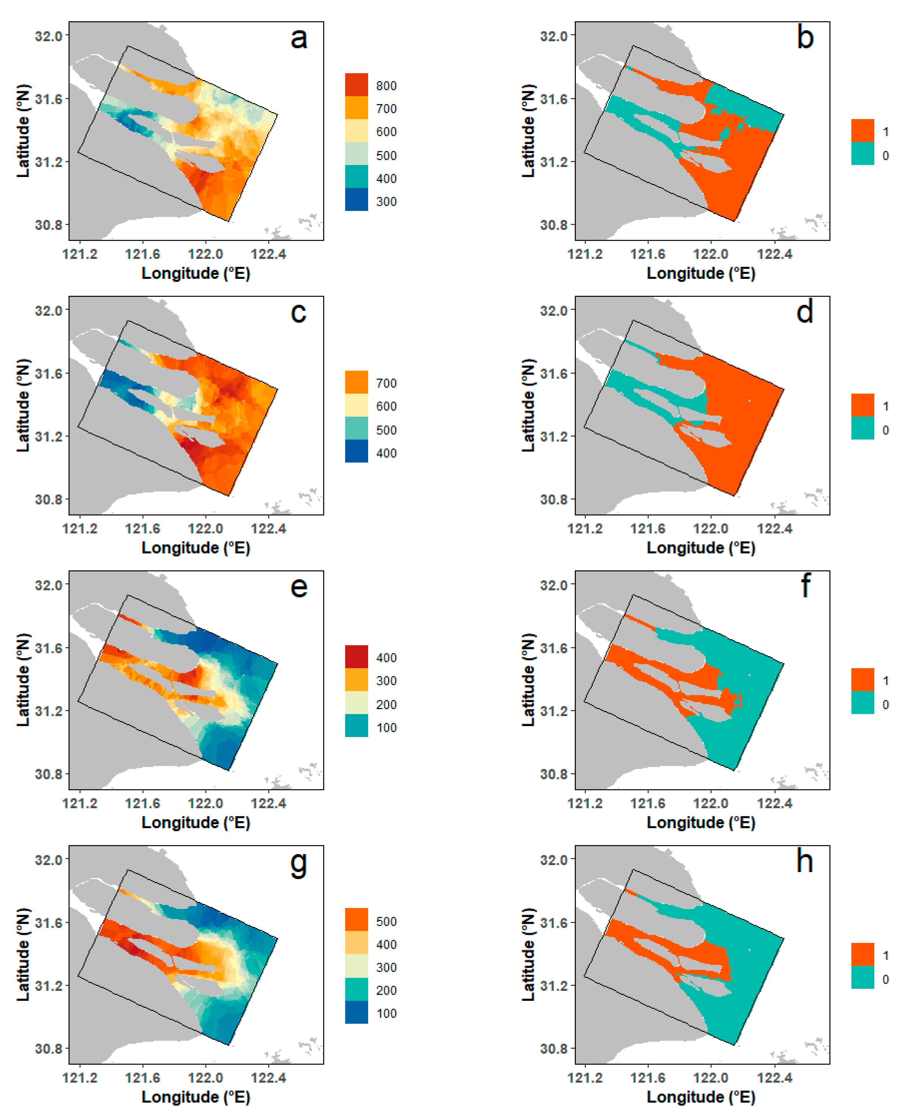
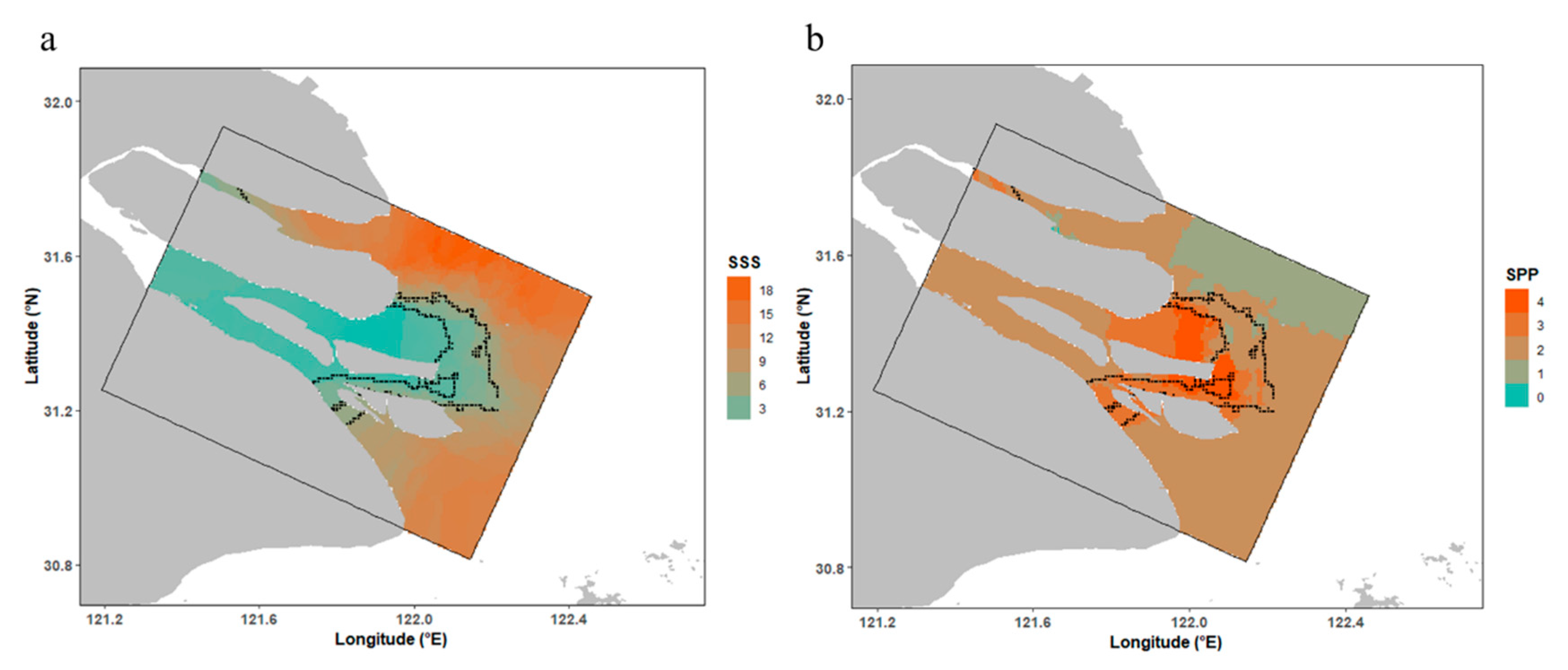
3.3. Spatial Patterns of Habitat Suitability

Our results showed that the brackish water guild species (C. mystus) and marine guild species (E. japonicus) are expected to have high habitat suitability outside the mouth of the Yangtze Estuary (east of 122° E), and that the freshwater guild species (P. sinensis and H. bleekeri) are expected to be present inside the mouth of the estuary (west of 122° E) (Figure 5 and Figure S1). The ensemble SDM indicated that C. mystus will most likely be found inside the North Branch (west of 122° E), Eastern Chongming, and outside the South Branch (east of 121.8° E), with an area of 2910.55 km2. The predicted environmentally suitable area (3460.68 km2) for E. japonicus was relatively larger than the area for C. mystus, which extended to outside the North Branch. For the two freshwater guild species, the suitable areas were generally similar and were mainly located inside the South Branch. The area for P. sinensis (1615.93 km2) was relatively larger than that for H. bleekeri (1136.87 km2).
We found that the area inside the South Branch and the other areas were divided into two different habitat types with low and high salinity (Figure 5 and Figure 6). A confluence of salt and fresh waters (Figure 6a), with SSS in the range of 2–5, occurs between these two areas [18]. In this mixing zone, we found an obvious overlapping distribution of the three ecological guild species (Figure 6b and Figure S2).

4. Discussion

4.1. Model Performances

Many studies have used the ensemble model to predict the habitats of marine species of different forms, including fish and crabs [55,56]. We found that ensemble SDMs for the four larval fish species exhibited predictive abilities superior to those of single algorithms, and that they had markedly increased the model’s accuracy, regardless of the database used. Especially for E. japonicus, only the RF algorithm in the single model was generally satisfactory for the performance statistics, whereas the ensemble model had increased the prediction ability of the model with values of 0.945 AUC and 0.740 TSS. The high phenotypic plasticity of E. japonicus perhaps influenced the prediction performance of the other single models [57]. Although higher AUC and TSS values were shown by the ensemble model, the performance of the ensemble models for DES larval fishes was different, especially for two freshwater species (Table 2). The model’s accuracy (0.928 AUC and 0.749 TSS) of P. sinensis was higher than that of H. bleekeri (0.899 AUC and 0.641 TSS). The distribution of freshwater species is concentrated in the freshwater region of the Southern Branch and the different distribution area may be the reason that affected the performance of the model. Although the accuracy of the models remarkably increased due to the application of ensemble methods emphasizing the “signal” emerging from different model outputs, this ensemble method will still depend on the accuracy of the single algorithms they are based on [40]. Thus, researchers still need to focus on the critical underlying issues of the single model to enhance the reliable prediction of species distributions. Moreover, in order to reduce the complexity of processing, we validated the models by using only the independent datasets (30% of our dataset). However, using cross-validation rather than simply splitting the data when assessing model performance could avoid the possibility of overestimating the predictive power of the models [58].
Ensemble models have been applied to avoid the necessity of selecting a single best model among many that may be approximately equivalent and may have potential errors due to overfitting [48]. In this study, we found that the RF algorithm showed stronger predictive abilities for all four larval fish than any other single algorithm. Although GLM and GAM may be the most traditional statistical models for predicting species distributions, they showed inferior performance compared with the nonlinear statistical models (especially the RF algorithm) [42]. The SRE algorithm was scarcely inaccurate in comparison with other methods.; thus, its use in the modeling of species distribution was doubted [56]. MaxEnt showed a low predictive power and stability, despite being one of the most widely used modeling techniques [22]. These results provide support for the arguments of enhanced performance consistently obtained for machine-learning techniques such as RF [42].

4.2. Environmental Variable Predictors

Salinity is a key environmental variable contributing to spatiotemporal variability in the assemblage structure of fish in estuaries [25,26,59]. We found that all DES were deeply influenced by salinity in the estuary. This is consistent with the results of previous studies, which showed that salinity mainly influenced the composition and abundance of most estuarine species [19]. Jiang et al. (2006) suggested that salinity changes influenced the distribution of larval fish, and the oligohaline region in the offshore had a significant impact on the hatching and development of larval fish in the Yangtze Estuary [60]. The rhythm of the river flow and the physiography of the estuary are the major factors that lead to the gradient variance and annual change in salinity [13,61]. We found obvious annual differences in the SSS, and the SSS in 2021 was the lowest (Table S1 Additionally, Figure S2). The Yangtze River flows in May in 2019, 2020, and 2021 were 92.4, 59.7, and 112.2 billon m3, respectively. We acquired the Yangtze River flow data that were measured at Datong station in May (117°37′ E, 30°46′ N) from the Changjiang Water Resources Commission of the Ministry of Water Resources (http://www.cjw.gov.cn, accessed on 16 January 2022). The evolution of saltwater intrusion can also influence the gradient variance of salinity due to the special topography of the Yangtze Estuary [62]. In the Yangtze Estuary, lower values of salinity are recorded in the South Branch, as opposed to high values of salinity in the North Branch [30]. The higher SSS inside the North Branch indicated that a stronger saline intrusion may have occurred in 2019 (Figure S2). Low salinity (SSS < 3) was unsuitable for the marine species (E. japonicus), but it was suitable for the freshwater species (P. sinensis and H. bleeker). Therefore, DES will select zones with different salinities as their nursery ground. The SSS suitable range for C. mystus (brackish water species) was 5–10 and 12–20. Hu et al. (2021) indicated that the suitable salinity of C. mystus larvae was 5–12 in the Yangtze Estuary (West of 122° E) by using the GAM model; they also reported that its distribution was more inclined to the North Branch with the higher salinity [63]. Due to the differences in the survey areas, our results can be used as a supplement to previous studies. Even though the mean salinity was low in 2021, E. japonicus could still maintain a broad distribution with phenotypic plasticity [57].
Multiple physical or chemical factors can also influence the distribution of larval fish species [7,17]. We found that E. japonicus belonged to the marine ecological guild and was deeply influenced by depth, whereas the distribution of the other species was not sensitive to depth. Hence, marine species may have higher requirements for depth [9]. Wan et al. (2002) showed that the spawning ground of E. japonicus gradually transferred from offshore Qingdao to deep-water areas in the south of the Yellow Sea [64]. Moreover, temperature was the key environmental variable affecting fish in many ways, including spawning, migration, and diet [26,30,57]. Most fish spawn in temperatures higher than 18 °C in the Yangtze Estuary [33]. Our results showed that temperate was the second key factor influencing the distribution of C. mystus and P. sinensis larval fish, but H. bleekeri, which also belongs to freshwater species, had little correlation with temperature. The SST suitable ranges for C. mystus were 20.5–21.8 °C and higher than 22.5 °C. The temperature rise might increase the recruitment success of C. mystus [30]. Thus, the temperature rise may be the reason why the abundance of C. mystus increased in 2020 and 2021 (Table 1). Moreover, we should notice that some potential factors, such as time-lagged (e.g., one month prior) SST and chlorophyll-a concentration, may also affected the distributions of larval fish species. In some cases, marine processes are better explained by time-lagged ecological variables, such as surface temperature, rather than simultaneous values [65]. Chlorophyll is often considered to have a 30-day accumulation period prior to being reflected in higher trophic levels through ocean food chains [66,67]. Thus, future research can focus on the lag of the environmental factors affecting the larval fish habitats.

4.3. Potential Habitat Description

This study on the distribution of DES will be helpful to understand the mechanism of fish habitat selection in estuaries. The four species that we considered are common species in the Yangtze Estuary and have considerable ecological and economic importance. Their larvae are important fishery resources and play an important role in the food web, and they are abundant in the study area [28,68]. Moreover, they use the estuary in different ways, which may explain the differences in the environmental tolerance and the different impacts of environmental variables on their distributions [5,9]. C. mystus, which is recognized as a brackish water species, is an estuarine migratory fish that commonly lives in shallow marine habitats but migrates to brackish estuarine waters and even freshwater areas in the spring as sexually mature individuals [23]. The main spawning period and location of C. mystus are spring and the South Branch of the Yangtze Estuary in China, respectively [14,30,69]. We found that the C. mystus larval fish were mainly distributed inside the North Branch and outside the South Branch. Thus, further studies are needed to understand the transport mechanism between the spawning and nursery ground of C. mystus. It may be closely related to hydrodynamic processes (e.g., the Yangtze River runoff), and geographic attachment may be the consequence of the recurrence of favorable conditions at particular locations [70,71]. The Japanese anchovy (E. japonicus) has been widely studied in biology, population variety, and ecology fields [57,72,73]. Kim et al. (2005) found that anchovy larvae peaked in May and June and that the distribution pattern was influenced by the monsoon season and Yangtze River discharge [72]. Iseki and Kiyomoto (1997) classified the Japanese anchovy population into two groups: one of the two groups was strongly characterized by a high concentration of anchovy ichthyoplankton in the low-salinity and high-turbidity areas at the frontal zone of the Yangtze River plume [74]. Our results corroborated this finding, as we found that the suitable habitat of Japanese anchovy larval fish was all areas except for the freshwater area in our study area. Although freshwater species are also an important part of the fish community in the Yangtze Estuary, researchers have paid little attention to the distribution of freshwater species in the Yangtze Estuary. We found that freshwater species were mainly distributed inside the South Branch. The distribution area for P. sinensis (1615.93 km2) was relatively larger than that of H. bleekeri (1136.87 km2).
Moreover, our results showed that the confluence of salt- and freshwater is a place where multiple ecological guild species coexist. According to the salinity gradient of the Yangtze Estuary, a previous study divided the Yangtze Estuary into four water systems and assigned one of the four water systems as the estuarine water because the salinity was in the range of one to five [18]. Considering the change in the estuarine environment, we assigned the SSS in the range of 2–5 as the confluence of salt- and freshwater. One possible reason for this result is that hydrodynamic processes (eddies) are an opportunity to adaptively respond, giving a competitive advantage for the larval fish [75]. Another possible reason is that the confluence of salt- and freshwater is the main factor controlling the nutrient distribution. The nutrient gradient formed in the process of mixing salt- and freshwater can cause differences in the growth degree and rate of phytoplankton and can change the nutrient structure of seawater due to local phytoplankton blooms [76,77]. There is an assumption that if the salinity gradient changes, the distribution pattern of the confluence of salt- and freshwater in the Yangtze Estuary will be shifted. This salinity gradient may be the reason why many fish species, particularly marine species, selected the estuary.
Our study suggests that the different distribution patterns were shown in DES larval fishes and the conservation activities should consider this aspect. Thus, there may be not a single conservation strategy to protect the total larval fish resource in the Yangtze Estuary. Adaptive conservation strategies for DES larval fish should take our findings into account. Species-specific conservation measures, such as species-specific fishing moratoriums (i.e., closure dates and closure areas), should be considered. At present, a long-term fishing ban strategy has been taken in the Yangtze Estuary by the Chinese government since 2020 for the purpose of protecting the estuarine fisheries resources. This may play an important role in the recovery of fishery resources in the Yangtze Estuary. Moreover, to maximize the benefits of conservation strategies, annual larval fish surveys should help clarify variations in the life-history traits of DES.

5. Conclusions

In this study, we explored spring suitable habitats for DES larval fish and examined the relationships between the presence of four species and environmental variables by using ensemble SDMs in the Yangtze Estuary. Nevertheless, our modeling approaches still have some limitations. First, we should note that we only included the presence/absence data and not the abundance data in our model. Therefore, it is impossible to confirm whether the confluence of salt- and freshwater also has abundant fish larvae. Second, the sample size may affect how well SDMs perform; increasing the amount of survey data will be beneficial to increase the model accuracy. However, long-term surveys in the Yangtze Estuary are difficult to conduct because of the fishing ban placed by the Chinese government (west of 122°15′ E).
The Yangtze Estuary is a very important region as it acts as a nursery ground for fish species, and many researchers have examined the larval fish assemblage structure in this area. Compare to other literatures on the Yangtze Esturay, we paid attention to high resolution samples to study the larval suitable habitats so that we could record various DES. This study provides the first set of published information on the relationship between the three ecological guild species and the surrounding environment in the Yangtze Estuary. Thus, the findings of this study will serve as a baseline against which future trends can be evaluated for the species, especially the freshwater species. Our findings suggest that environmental variables likely determine the spatial distribution pattern of the DES larval fish and that salinity is a key variable that contributes to their spatial variability. Consequently, no single conservation strategy to protect the total larval fish resources in our study area may exist. Species-specific conservation measures should be considered based on our study.

Supplementary Materials

The following supporting information can be downloaded at: https://www.mdpi.com/article/10.3390/fishes8040209/s1, Figure S1: The distribution of modeled and observed for the four model species in all three cruises in the Yangtze Estuary. ((a–c) C. mystus; (d–f) E. japonicas; (g–i) P. sinensis; (j–l) H. bleekeri); Figure S2: The spatial patterns of SSS (a) and the sum of predicted presences of the four species (b) considered in all three cruises in the Yangtze Estuary; Table S1: Mean total values for depth (Dep, m), sea surface temperature (SST, °C), sea surface salinity (SSS), sea surface chlorophyll a (SSChl, mg/m3) sampled from three cruises in Yangtze Estuary (±95% confidence interval).

Author Contributions

Conceptualization, R.W. and Z.L.; investigation, X.L., D.W. and L.Z.; writing original draft, P.S.; writing, review and editing, Z.L. All authors have read and agreed to the published version of the manuscript.

Funding

This study was supported by Shanghai Municipal Science and Technology Commission Local Capacity Construction Project (grant No. 21010502200), Science and Technology Commission of Shanghai Municipality (grant No. 22YF1416500).

Institutional Review Board Statement

Not applicable.

Informed Consent Statement

Informed consent was obtained from all subjects involved in the study.

Data Availability Statement

Data is unavailable due to privacy restrictions.

Acknowledgments

We thank our colleagues for their contributions to data collection and laboratory experiments.

Conflicts of Interest

The authors declare that they have no known competing financial interest or personal relationships that could have appeared to influence the work reported in this paper.

References

  1. Miller, B.S.; Kendall, A.W. Development of eggs and larvae. In Early Life History of Marine Fishes; University of California Press: Berkeley, CA, USA, 2009; pp. 39–54. [Google Scholar]
  2. Branch, G. Estuarine vulnerability and ecological impacts. In Estuaries of South Africa; Allanson, B.R., Baird, D., Eds.; Cambridge University Press: Cambridge, UK, 1999; p. 340. [Google Scholar]
  3. Kennish, M.J. Environmental threats and environmental future of estuaries. Environ. Conserv. 2002, 29, 78–107. [Google Scholar] [CrossRef]
  4. Lewis, L.J.; Davenport, J.; Kelly, T.C. A study of the impact of a pipeline construction on estuarine benthic invertebrate communities. Part 2. Recolonization by benthic invertebrates after 1 year and response of estuarine birds. Estuar. Coast. Shelf Sci. 2003, 47, 201–208. [Google Scholar] [CrossRef]
  5. Potter, M.; Whitfield, A.K.; Potter, I.C.; Blaber, S.J.M.; Cyrus, D.P.; Nordlie, F.G.; Harrison, T.D. The guild approach to categorizing estuarine fish assemblages: A global review. Fish Fish. 2007, 8, 241–268. [Google Scholar]
  6. Beck, M.W.; Heck, K.L.; Able, K.W.; Childers, D.L.; Eggleston, D.B.; Gillanders, B.M.; Halpern, B.; Hays, C.G.; Hoshino, K.; Minello, T.J. The identification, conservation, and management of estuarine and marine nurseries for fish and invertebrates. BioScience. 2009, 51, 633–641. [Google Scholar] [CrossRef]
  7. Vanhatalo, J.; Veneranta, L.; Hudd, R. Species distribution modeling with Gaussian processes: A case study with the youngest stages of sea spawning whitefish (Coregonus lavaretus L. sl) larvae. Ecol. Model. 2012, 228, 49–58. [Google Scholar] [CrossRef]
  8. Long, X.Y.; Wan, R.; Li, Z.G.; Ren, Y.P.; Song, P.B.; Tian, Y.J.; Xu, B.D.; Xue, Y. Spatio-temporal distribution of Konosirus punctatus spawning and nursing ground in the South Yellow Sea. Acta Oceanol. Sin. 2021, 40, 133–144. [Google Scholar] [CrossRef]
  9. Potter, I.C.; Tweedley, J.R.; Elliott, M.; Whitfield, A.K. The ways in which fish use estuaries: A refinement and expansion of the guild approach. Fish Fish. 2015, 16, 230–239. [Google Scholar] [CrossRef]
  10. Hernández-Miranda, E.; Palma, A.T.; Ojeda, F.P. Larval fish assemblages in nearshore coastal waters off central Chile: Temporal and spatial patterns. Estuar. Coast. Shelf Sci. 2003, 56, 1075–1092. [Google Scholar] [CrossRef]
  11. Bento, E.G.; Grilo, T.F.; Nyitrai, D.; Dolbeth, M.; Pardal, M.A.; Martinho, F. Climate influence on juvenile European sea bass (Dicentrarchus labrax, L.) populations in an estuarine nursery: A decadal overview. Mar. Environ. Res. 2016, 122, 93–104. [Google Scholar] [CrossRef]
  12. Guerreiro, M.A.; Martinho, F.; Baptista, J.; Costa, F.; Pardal, M.A.; Primo, A.L. Function of estuaries and coastal areas as nursery grounds for marine fish early life stages. Mar. Environ. Res. 2021, 170, 105408. [Google Scholar] [CrossRef]
  13. Barletta, M.; Barletta-Bergan, A.; Saint-Paul, U.; Hubold, G. The role of salinity in structuring the fish assemblages in a tropical estuary. J. Fish. Bio. 2005, 66, 45–72. [Google Scholar] [CrossRef]
  14. Zhuang, P.; Wang, Y.; Li, S.; Deng, S.; Li, C.; Ni, Y. Fishes of the Yangtze Estuary; Shanghai Scientific & Technical Publishers: Shanghai, China, 2006. (In Chinese) [Google Scholar]
  15. Elliott, M.; Whitfield, A.K. Challenging paradigms in estuarine ecology and management. Estuar. Coast. Shelf Sci. 2011, 94, 306–314. [Google Scholar] [CrossRef]
  16. Leskelä, A.; Hudd, R.; Lehtonen, H.; Huhmarniemi, A.; Sandstrm, O. Habitats of whitefish (Coregonus lavaretus (L.) s.l.) larvae in the Gulf of Bothnia. Aqua. Fennica. 1991, 21, 145–151. [Google Scholar]
  17. Pattrick, P.; Strydom, N.A.; Harris, L.; Goschen, W.S. Predicting spawning locations and modelling the spatial extent of post hatch areas for fishes in a shallow coastal habitat in South Africa. Mar. Ecol. Prog. Ser. 2016, 560, 223–235. [Google Scholar] [CrossRef]
  18. Hu, F.X.; Hu, H.; Gu, G.W.; Su, C.; Gu, X.J. Salinity front in the Changjiang estuary. Oceanol. Limnol. Sin. Supplement. 1995, 26, 23–31. (In Chinese) [Google Scholar]
  19. Whitfield, A.K. Estuaries-how challenging are these constantly changing aquatic environments for associated fish species? Environ. Biol. Fish. 2021, 104, 517–528. [Google Scholar] [CrossRef]
  20. Vasconcelos, R.P.; Le Pape, O.; Costa, M.J.; Cabral, H.N. Predicting estuarine use patterns of juvenile fish with generalized linear models. Estuar. Coast. Shelf Sci. 2013, 120, 64–74. [Google Scholar] [CrossRef]
  21. Zhang, Z.X.; Xu, S.Y.; Capinhac, C.; Weteringsd, R.; Gao, T.X. Using Species Distribution Model to Predict the Impact of Climate Change on the Potential Distribution of Japanese Whiting Sillago Japonica. Ecol. Indic. 2019, 104, 333–340. [Google Scholar] [CrossRef]
  22. Zhao, G.H.; Cui, X.Y.; Sun, J.J.; Li, T.T.; Wang, Q.; Ye, X.Z.; Fan, B.G. Analysis of the distribution pattern of chinese ziziphus jujuba under climate change based on optimized biomod2 and maxent models. Ecol. Indic. 2021, 132, 108256. [Google Scholar] [CrossRef]
  23. He, W.; Li, Z.; Liu, J.; Li, Y.; Murphy, B.R.; Xie, S. Validation of a method of estimating age, modelling growth, and describing the age composition of Coilia mystus from the Yangtze Estuary, China. ICES J. Mar. Sci. 2008, 65, 1655–1661. [Google Scholar] [CrossRef]
  24. Yang, D.L.; Wu, G.Z.; Sun, J.R. The investigation of pelagic eggs, larvae and juveniles of fishes at the mouth of the Changjiang River and adjacent areas. Oceanol. Limnol. Sin. 1990, 21, 346–354. (In Chinese) [Google Scholar]
  25. Zhang, H.; Xian, W.W.; Liu, S.D. Autumn ichthyoplankton assemblage in the Yangtze Estuary shaped by environmental factors. PeerJ 2016, 4, e1922. [Google Scholar] [CrossRef]
  26. Zhang, H.; Xian, W.W.; Liu, S.D. Ichthyoplankton assemblage structure of springs in the Yangtze Estuary revealed by biological and environmental visions. PeerJ 2015, 3, e1186. [Google Scholar] [CrossRef]
  27. Yu, W.J.; Shen, J.Z.; Gong, J.; Li, Q.; Li, C.S.; Wang, K.X.; Mei, Z.G. Reproductive biology of Hemiculter bleekeri in the middle reaches of the Yangtze River. Freshw. Fish. 2018, 48, 53–60. (In Chinese) [Google Scholar]
  28. Wan, R.; Song, P.; Li, Z.; Long, X.; Wang, D.; Zhai, L. Larval Fish Spatiotemporal Dynamics of Different Ecological Guilds in Yangtze Estuary. J. Mar. Sci. Eng. 2023, 11, 143. [Google Scholar] [CrossRef]
  29. Ruan, H.T.; Xu, S.N.; Li, M.; Dai, J.G.; Li, Z.H.; Zou, K.S.; Liu, L. Microsatellite primers screening and genetic diversity analysis of five geographical populations of Pseudolaubuca sinensis in the pearl river basin. Acta Hydrobio. Sin. 2020, 44, 501–508. (In Chinese) [Google Scholar]
  30. Wang, D.; Wan, R.; Li, Z.G.; Zhang, J.B.; Long, X.Y.; Song, P.B.; Zhai, L.; Zhang, S. The Non-stationary Environmental Effects on Spawning Habitat of Fish in Estuaries: A Case Study of Coilia mystus in the Yangtze Estuary. Front. Mar. Sci. 2021, 8, 766616. [Google Scholar] [CrossRef]
  31. Zhang, Z.X.; Mammola, S.; Xian, W.W.; Zhang, H. Modelling the potential impacts of climate change on the distribution of ichthyoplankton in the Yangtze Estuary, China. Divers. Distrib. 2020, 26, 126–137. [Google Scholar] [CrossRef]
  32. Ma, J.; Huang, J.L.; Chen, J.H.; Li, B.; Zhao, J.; Gao, C.X.; Wang, X.F.; Tian, S.Q. Analysis of spatiotemporal fish density distribution and its influential factors based on generalized additive model (GAM) in the Yangtze River Estuary. Chin. J. Fish. 2020, 44, 936–946. (In Chinese) [Google Scholar]
  33. Kindong, R.; Chen, J.H.; Dai, L.B.; Gao, C.X.; Han, D.Y.; Tian, S.Q.; Wu, J.H.; Ma, Q.Y.; Tang, J.Y. The effect of environmental conditions on seasonal and inter-annual abundance of two species in the Yangtze River estuary. Mar. Freshw. Res. 2021, 72, 493–506. [Google Scholar] [CrossRef]
  34. Guisan, A.; Zimmerman, N.E. Predictive habitat distribution models in ecology. Ecol. Model. 2000, 135, 147–186. [Google Scholar] [CrossRef]
  35. Araújo, M.B.; New, M. Ensemble forecasting of species distributions. Trends Ecol. Evol. 2007, 22, 42–47. [Google Scholar] [CrossRef]
  36. Elith, J.; Leathwick, J.R. Species distribution models: Ecological explanation and prediction across space and time. Annu. Rev. Ecol. Evol. Syst. 2009, 40, 677–697. [Google Scholar] [CrossRef]
  37. Franklin, J. Mapping Species Distributions: Spatial Inference and Prediction; Cambridge University Press: Cambridge, UK, 2010. [Google Scholar]
  38. Bacheler, N.M.; Ciannelli, L.; Bailey, K.M.; Anderson, J.T. Spatial and temporal patterns of walleye pollock (Theragra chalcogramma) spawning in the eastern Bering Sea inferred from egg and larval distributions. Fish. Oceanogr. 2010, 19, 107–120. [Google Scholar] [CrossRef]
  39. Li, Z.G.; Wan, R.; Ye, Z.J.; Chen, Y.; Ren, Y.P.; Liu, H.; Jiang, Y.Q. Use of random forests and support vector machines to improve annual egg production estimation. Fish. Sci. 2017, 83, 1–11. [Google Scholar] [CrossRef]
  40. Franca, S.; Cabral, H.N. Distribution models of estuarine fish species: The effect of sampling bias, species ecology and threshold selection on models’ accuracy. Ecol. Inform. 2019, 51, 168–176. [Google Scholar] [CrossRef]
  41. Thuiller, W. BIOMOD–optimizing predictions of species distributions and projecting potential future shifts under global change. Global Change Biol. 2003, 9, 1353–1362. [Google Scholar] [CrossRef]
  42. Li, Z.G.; Ye, Z.J.; Wan, R.; Zhang, C. Model selection between traditional and popular methods for standardizing catch rates of target species: A case study of Japanese Spanish mackerel in the gillnet fishery. Fish. Res. 2015, 161, 312–319. [Google Scholar] [CrossRef]
  43. Thuiller, W.; Georges, D.; Engler, R.; Breiner, F. biomod2: Ensemble Platform for Species Distribution Modeling; R Package: Vienna, Austria, 2016; Available online: https://CRAN.R-project.org/package=biomod2 (accessed on 1 January 2020).
  44. Zhang, R.Z.; Lu, H.F. Eggs and Larvae in the Offshore of China; Shanghai Scientific & Technical Publishers: Shanghai, China, 1985. (In Chinese) [Google Scholar]
  45. Qiao, Y. Early Morphogenesis and Species Identification of Fishes in Yangtze River; Institute of Hydrobiology, Chinese Academy of Science: Wuhan, China, 2005. (In Chinese) [Google Scholar]
  46. Arranz, I.; Mehner, T.; Benejam, L.; Argillier, C.; Holmgren, K.; Jeppesen, E.; Lauridsen, T.L.; Volta, P.; Winfield, I.J.; Winfield, S. Density-dependent effects as key drivers of intraspecific size structure of six abundant fish species in lakes across Europe. Can. J. Fish. Aquat. Sci. 2016, 73, 519–534. [Google Scholar] [CrossRef]
  47. Fletcher, D.H.; Gillingham, P.K.; Britton, J.R.; Blanchet, S.; Gozlan, R.E. Predicting global invasion risks: A management tool to prevent future introductions. Sci. Rep. 2016, 6, 26316. [Google Scholar] [CrossRef]
  48. Thuiller, W.; Guéguen, M.; Renaud, J.; Karger, D.N.; Zimmermann, N.E. Uncertainty in ensembles of global biodiversity scenarios. Nat. Commun. 2019, 10, 1446. [Google Scholar] [CrossRef]
  49. Allouche, O.; Tsoar, A.; Kadmon, R. Assessing the accuracy of species distribution models: Prevalence, kappa and the true skill statistic (TSS). J. Appl. Ecol. 2006, 43, 1223–1232. [Google Scholar] [CrossRef]
  50. Wang, Y.S.; Xie, B.Y.; Wan, F.H.; Xiao, Q.M.; Dai, L.Y. Application of ROC curve analysis in evaluating the performance of alien species’ potential distribution models. Biodivers. Sci. 2007, 4, 365–372. (In Chinese) [Google Scholar]
  51. Hijmans, R.J. Raster: Geographic Data Analysis and Modeling; R Package: Vienna, Austria, 2014; Available online: http://CRAN.R-project.org/package=raster (accessed on 1 January 2020).
  52. Hijmans, R.J. Terra: Spatial Data Analysis; R Package: Vienna, Austria, 2023; Available online: http://CRAN.R-project.org/package=terra (accessed on 1 January 2020).
  53. Deckmyn, A. Maps: Draw Geographical Maps; R Package: Vienna, Austria, 2022; Available online: http://CRAN.R-project.org/package=maps (accessed on 1 January 2020).
  54. Ginestet, C. ggplot2: Elegant Graphics for Data Analysis. J. R. Stat. Soc. 2011, 174, 245–246. [Google Scholar] [CrossRef]
  55. Liu, X.Y.; Han, X.L.; Han, Z.Q. Effects of Climate Change on the Potential Habitat Distribution of Swimming Crab (Portunus trituberculatus) under the Species Distribution Model. J. Oceanol. Limnol. 2022, 40, 1556–1565. [Google Scholar] [CrossRef]
  56. Yang, T.Y.; Liu, X.Y.; Han, Z.Q. Predicting the Effects of Climate Change on the Suitable Habitat of Japanese Spanish Mackerel (Scomberomorus niphonius) Based on the Species Distribution Model. Front. Mar. Sci. 2022, 9, 927790. [Google Scholar] [CrossRef]
  57. Zhang, W.; Yu, H.; Ye, Z.; Tian, Y.; Liu, Y.; Li, J.; Jiang, Y. Spawning strategy of Japanese anchovy Engraulis japonicus in the coastal Yellow Sea: Choice and dynamics. Fish. Oceanogr. 2020, 30, 366–381. [Google Scholar] [CrossRef]
  58. Wenger, S.J.; Olden, J.D. Assessing transferability of ecological models: An underappreciated aspect of statistical validation. Methods Ecol. Evol. 2012, 3, 260–267. [Google Scholar] [CrossRef]
  59. Whitfield, A.K.; Elliott, M.; Basset, A.; Blader, S.J.M.; West, R.J. Paradigms in the estuarine ecology: A review of the Remane diagram with a suggested revised model for estuaries. Estuar. Coast. Shelf Sci. 2012, 97, 78–90. [Google Scholar] [CrossRef]
  60. Jiang, M.; Shen, X.Q.; Wang, Y.L.; Yuan, Q.; Chen, L.F. Species of fish eggs and larvae and distribution in Changjiang Estuary and vicinity waters. Acta Oceanol. Sin. 2006, 28, 171–174. (In Chinese) [Google Scholar]
  61. Sun, T.; Yang, Z.F.; Shen, Z.Y.; Zhao, R. Environmental flows for the Yangtze estuary based on salinity objectives. Commun. Nonlinear Sci. 2009, 14, 959–971. [Google Scholar] [CrossRef]
  62. Li, L.; Zhu, J.R.; Wu, H. Impacts of wind stress on saltwater intrusion in the Yangtze Estuary. Sci. China Earth Sci. 2012, 55, 1178–1192. [Google Scholar] [CrossRef]
  63. Hu, L.J.; Song, C.; Geng, Z.; Zhao, F.; Jiang, J.; Liu, R.H.; Zhuang, P. Temporal and spatial distribution of Coilia mystus larvae and juveniles in the Yangtze Estuary during primary breeding season. J. Chin. Fish. Sci. 2021, 28, 1152–1161. (In Chinese) [Google Scholar]
  64. Wan, R.J.; Huang, D.J.; Zhang, J. Abundance and distribution of eggs and larvae of Engraulis japonicus in the Northern part of East China Sea and the Southern part of Yellow Sea and its relationship with environmental conditions. J. Chin. Fish. 2002, 26, 321–330. [Google Scholar]
  65. Olden, J.D.; Neff, B.D. Cross-correlation bias in lag analysis of aquatic time series. Mar. Biol. 2001, 138, 1063–1070. [Google Scholar] [CrossRef]
  66. Trujillo, A.P.; Thurman, H.V. Essentials of Oceanography, 12th ed.; Pearson Education, Inc.: Boston, MA, USA, 2016; pp. 403–444. [Google Scholar]
  67. Wang, L.; Kerr, L.A.; Record, N.R.; Bridger, E.; Tupper, B.; Mills, K.E.; Armstrong, E.M.; Pershing, A.J. Modeling marine pelagic fish species spatiotemporal distributions utilizing a maximum entropy approach. Fish. Oceanogr. 2018, 27, 571–586. [Google Scholar] [CrossRef]
  68. Rao, Y.Y. Study on Annual Resource Variation of Larvae and Juveniles in the Southern Branch of the Yangtze River Estuary; Shanghai Ocean University: Shanghai, China, 2022. (In Chinese) [Google Scholar]
  69. Ni, Y.; Wang, Y.L.; Jiang, M.; Chen, Y.Q. Biological characteristics of Coilia mystus in the Changjiang estuary. J. Fish. Sci. 1999, 6, 69–71. (In Chinese) [Google Scholar]
  70. Reglero, P.; Ciannelli, L.; Alvarez-Berastegui, D.; Balbín, R.; Alemany, F. Geographically and environmentally driven spawning distributions of tuna species in the western Mediterranean Sea. Mar. Ecol. Prog. Ser. 2012, 463, 273–284. [Google Scholar] [CrossRef]
  71. Brunel, T.; van Damme, C.J.G.; Samson, M.; Dickey-Collas, M. Quantifying the influence of geography and environment on the northeast Atlantic mackerel spawning distribution. Fish. Oceanogr. 2017, 27, 159–173. [Google Scholar] [CrossRef]
  72. Kim, J.Y.; Kang, Y.S.; Oh, H.; Suh, Y.S.; Hwang, J.D. Spatial distribution of early life stages of anchovy (Engraulis japonicus) and hairtail (Trichiurus lepturus) and their relationship with oceanographic features of the East China Sea during the 1997–1998 El Niño Event. Estuar. Coast. Shelf Sci. 2005, 63, 13–21. [Google Scholar] [CrossRef]
  73. Ito, Y.; Yasuma, H.; Masuda, R.; Minami, K.; Matsukura, R.; Morioka, S.; Miyashita, K. Swimming angle and target strength of larval Japanese anchovy (Engraulis japonicus). Fish. Sci. 2011, 77, 161–167. [Google Scholar] [CrossRef]
  74. Iseki, K.; Kiyomoto, Y. Distribution settling of Japanese anchovy (Englaulis japonicus) eggs at the spawning ground off Changjing river in the East China sea. Fish. Oceanogr. 1997, 6, 205–210. [Google Scholar] [CrossRef]
  75. BaKun, A. Fronts and eddies as key structures in the habitat of marine fish larvae: Opportunity, adaptive response and competitive advantage. Sci. Mar. 2006, 70, 105–122. [Google Scholar] [CrossRef]
  76. Ning, X.R.; Shi, J.X.; Cai, Y.M.; Liu, C.G. Biological productivity front in the Changjiang Estuary and Hangzhou Bay and its ecological effects. Acta Oceanol. Sin. 2004, 26, 96–106. [Google Scholar]
  77. Wang, K.; Chen, J.F.; Li, H.L.; Jin, H.Y.; Xu, J.; Gao, S.Q.; Lu, Y.; Huang, D.J. The influence of freshwater-saline water mixing on phytoplankton growth in Changjiang Estuary. Acta Ecol. Sin. 2012, 32, 17–26. (In Chinese) [Google Scholar] [CrossRef]
Figure 1. Study area and samples in the Yangtze Estuary (a) represents the study area; (b) represents the samples. Black boxes represent study area in the present study; points represent sampling stations).
Fishes 08 00209 g001
Figure 2. Predictive abilities of the ten modelling algorithms (artificial neural networks (ANN), classification tree analysis (CTA), flexible discriminant analysis (FDA), generalized additive model (GAM), generalized boosting model (GBM), generalized linear model (GLM), multiple adaptive regression splines (MARS), maximum entropy (MaxEnt), random forest (RF), and surface range envelop (SRE)) for the four larval fish. Dashed lines represent cutoff levels for the area under the receiver operating characteristic curve (AUC = 0.7) and true skill statistic (TSS = 0.4) used to select the algorithms to remain in the ensemble species distribution models (SDMs). Values are expressed as mean ± standard error.
Fishes 08 00209 g002
Figure 3. Importance of the four environmental variables (depth (Depth, m), sea surface temperature (SST, °C), sea surface salinity (SSS), and sea surface chlorophyll-a concentration (SSChl, mg/m3)) from the ensemble model for the four larval fish species.
Fishes 08 00209 g003
Figure 4. Response curves of explanatory variables (depth (Depth, m), sea surface temperature (SST, °C), sea surface salinity (SSS), and sea surface chlorophyll-a concentration (SSChl, mg/m3)) for the four larval fish species. ((ad) C. mystus; (eh) E. japonicus; (il) P. sinensis; (mp) H. bleekeri). Dashed lines represent cutoff levels by selecting a probability threshold that maximized the true skill statistic (TSS) value.
Fishes 08 00209 g004
Figure 5. Suitable habitat areas of the four larval fish species (The legends of (a,c,e,g) represent the projected habitat suitability values). The legends of (b,d,f,h) represent presence or absence in this area. ((a,b) C. mystus; (c,d) E. japonicus; (e,f) P. sinensis; (g,h) H. bleekeri).
Fishes 08 00209 g005
Figure 6. Spatial patterns of SSS (a) and the sum of predicted presences of the four species (b) considered in this study. Black-line region represents the confluence of salt and fresh waters. Map scale ranges from 0 (no species are predicted to be present) to 4 (all four species are predicted to be present). SSS, sea surface salinity; SPP, the sum of predicted presences.
Fishes 08 00209 g006
Table 1. Details of larval fish surveys and larval fish collection in the Yangtze Estuary.
Cruise TimingStationsNumber of Stations with Larval Fish Present (Number of Larval Fish)
C. mystusE. japonicusP. sinensisH. bleekeri
May 20195711 (2627)37 (25,406)1 (21)25 (734)
May 20205643 (40,572)30 (6399)18 (5509)17 (3106)
May 20215548 (25,379)42 (32,366)12 (26,027)13 (19,077)
Table 2. Predictive abilities of ensemble species distribution models (SDMs) for each larval fish species.
SpeciesAUCTSSCutoffSensitivity (%)Specificity (%)
C. mystus0.9380.766616.087.25587.897
E. japonicus0.9450.740677.080.73493.220
P. sinensis0.9280.749243.096.77478.102
H. bleekeri0.8990.641445.081.81882.301
Note: the AUC represents the area under the receiver operating characteristic curve; TSS represents the true skill statistic; Cutoff represents the projected habitat suitability values into present/absence (0/1) by selecting a probability threshold that maximized the TSS value. The sensitivity represents the proportion of the positive samples that were correctly classified. The specificity represents the proportion of the negative samples that were correctly classified.
Disclaimer/Publisher’s Note: The statements, opinions and data contained in all publications are solely those of the individual author(s) and contributor(s) and not of MDPI and/or the editor(s). MDPI and/or the editor(s) disclaim responsibility for any injury to people or property resulting from any ideas, methods, instructions or products referred to in the content.

