Article

Effects of Vertical Water Column Temperature on Distribution of Juvenile Tuna Species in the South China Sea

1
Third Institute of Oceanography, Ministry of Natural Resources, Xiamen 361005, China
2
College of Fisheries, Ocean University of China, Qingdao 266003, China
*
Authors to whom correspondence should be addressed.
Fishes 2023, 8(3), 135; https://doi.org/10.3390/fishes8030135
Submission received: 6 January 2023 / Revised: 10 February 2023 / Accepted: 22 February 2023 / Published: 26 February 2023
(This article belongs to the Section Biology and Ecology)

Abstract

:
In this study, we conducted two surveys in the central and southern parts of the South China Sea, in autumn 2012 and spring 2013. Six juvenile tuna species were caught in each survey. Gradient forest analysis (GFA) and a generalized additive model (GAM) were used to analyze the relationship between the catch per unit effort (CPUE) for the juvenile tuna species and six sea temperature indices for the South China Sea. In the GFA, the temperature difference between the sea surface and 50 m depth (D50) showed the highest importance to CPUE than other indices, which indicates that D50 was the best predictor of the abundance of juvenile tuna species. The GAM analysis showed that lower deep-water temperature, a shallow mixed layer depth, and a higher difference in temperature between the surface and deeper water were associated with increased CPUE. The results indicate that a relatively rapid decrease in vertical water temperature is favorable for the aggregation of juvenile tuna. These results contribute to understanding of the distribution mechanism of juvenile tuna species in the South China Sea and provide a scientific basis for the rational development and utilization of tuna resources.
Key Contribution: Relatively rapid decrease in vertical water temperature is favorable for the aggregation of juvenile tuna species.

1. Introduction

Tuna are the main fished species among the world’s pelagic fisheries, and are distributed in tropical and subtropical oceanic waters [1,2,3]. In the broad sense, tuna species include Thunnus having high economic value, but also tuna-like species having relatively low economic value, including Katsuwonus, Auxis [4]. Tuna species were one of the most valuable fishing classes, and they are considered to be an important contributor to global food security [5]. Tuna species are highly migratory and move between coastal ecosystems and the open ocean [6]. The Pacific Ocean is particularly important for tuna species, as it holds 70 percent of the total global catch [7]. The South China Sea is one of the five major tuna fishing grounds in the Pacific Ocean. Tuna are the main catch of longline fisheries in the South China Sea, accounting for approximately 60–70% of the total catch [8]. Countries adjacent to the South China Sea have been developing tuna fisheries for decades. Based on the stock assessment of Vietnam Research Institute of Marine Fisheries (RIMF), the abundance of tuna species in the western and central South China Sea were approximately 6.6 × 10⁵ tons [9,10].
The entire life history of marine fishes is closely related to the marine environment, especially for long-range migratory species including tuna, where the selection of migration routes and spawning grounds is largely influenced by the marine environment [11,12,13,14]. With increasing global climate change, the marine environment has undergone dramatic changes, including a significant increase in sea temperature, and these have important implications for fish distribution patterns [15,16,17]. Studies have shown that climatic and marine environmental changes have major effects on the distribution and abundance of tuna species [18,19,20,21,22,23]. Understanding how the environment affects the distribution of tuna species is fundamental to successful ecosystem-based management [3,24,25]. Juvenile tuna species are more vulnerable to the effects of the marine environment than adults. Assessments of the abundance of juvenile tuna are considered particularly crucial for effective stock management because these can be used to forecast recruitment and long-term population abundance [26].
Among various marine environmental factors, sea temperature is considered the most important one affecting fish distribution [27,28]. Some research points that tuna species are highly sensitive to changes in water temperature, and they can quickly move to cooler waters if the temperature rises too high [29]. The appropriate temperature can result in a lower metabolic rate and reduced energy costs, especially in areas where food is scarce [30]. Analysis of the spatial distribution of the nominal catch per unit effort by deep longline showed that the maximum aggregation of yellowfin tuna (Thunnus albacares) in waters with sea surface temperature (SST) above 24–25 °C [20]. It has also been proved that an increase in SST in the eastern Pacific Ocean leads to an increase in the production of tuna species [6]. Moreover, changes in SST in the Pacific Ocean can even affect changes in tuna stocks in the Indian Ocean [5,23]. Some research on the South China Sea tuna has also shown SST has a major influence on the distribution of tuna species [31,32]. Zhou et al. [32] used SST and sea surface height to establish a prediction model of yellowfin tuna in the South China Sea by using Bayes classifier, and the prediction accuracy of the model could reach 60%.
However, the relationship between juvenile tuna and water temperature has not been well-clarified. Adult tunas mainly occur in water depths of 50–500 m, while the juveniles are generally found at depths of around 50 m [22,33,34]. Therefore, using SST alone cannot fully explain the pattern of distribution of tuna species. To understand the distribution pattern of juvenile tuna species and the formation mechanism of their fishing grounds, it is necessary to more fully explore the effects of the marine environment on juvenile tuna species. In this study, the catch per unit effort (CPUE) of juvenile tuna species (an integrate over Thunnus. albacares, T. obesus, Katsuwonus pelamis, Auxis thazard, A. rochei, and Euthynnus yaito) in the South China Sea and six sea temperature indices were analyzed using gradient forest analysis (GFA) and a generalized additive model (GAM). The purpose of this study was to investigate the relationship between the vertical structure of the water column temperature above 100 m and the distribution of juvenile tuna species. The results can provide new insights into the distribution mechanism of juvenile tuna species and provide important support for forecast and effective management of tuna species stock in the South China Sea.

2. Materials and Methods

2.1. Fisheries Data

The fisheries data were obtained through two surveys, one in autumn (September to October) 2012 and the other in spring (March to April) 2013. The survey area is in the central and southern part of the South China Sea (5°25′–16°24′ N, 108°58′–117°31′ E); 42 stations were surveyed in 2012 and 43 in 2013 (Figure 1).
The same commercial fishing vessel (39.02 m length, 7.2 m width, 4.1 m draught, and 416 gross tonnage) was used in both surveys. Biological samples were collected at night using a light falling net. The net dimensions were 290.56 m in circumference and 85.12 m stretched length, and it had a 20 mm cod-end mesh and mesh of 35 mm at the net mouth. The maximum working depth of the net was 70 m. There were 230 attracting lamps (1 kw/lamp) arranged in two rows along the sides of the vessel.
The catch was sorted into species and randomly sampled. Standard measurements, including the fork length and body weight of all individuals, were recorded in the laboratory. Juvenile tuna species are defined as the fork length less than 40 cm [35,36,37]. The CPUE for each station was used as the abundance index for the juvenile tuna species. For light falling-nets, the fishing effort is mainly dependent on the duration of operation of the attracting lamps. Therefore, for each CPUE (kg/h) for juvenile tuna was calculated as the total catch of juvenile tuna (kg) divided by the duration of the light operation (h).

2.2. Environmental Data

Sea temperature data were obtained using a SV48 conductivity–temperature–depth (CTD) profiler produced by Sea & Sun Technology GmbH (Trappenkamp, Germany). The CTD profiler was placed deeper than 100 m at each station. The sea surface temperature (SST; 2 m depth), the sea temperature at 50 m depth (ST50), and the sea temperature at 100 m depth (ST100) were recorded separately, and the temperature differences between the SST and 50 m depth (D50), and the SST and 100 m depth (D100) were calculated. The mixed layer depth (MLD), calculated according to the method used for the South China Sea by Shi et al. (2001), was defined as the depth at which the temperature was 1 °C lower than the average temperature within 10 m of the surface layer [38].

2.3. Gradient Forests Analysis

In order to analyze the effect of vertical water column on distribution of juvenile tuna species, we used gradient forest (R package gradientForest; R Core Team, 2012) to quantitatively analyze the importance of environmental factors (SST, ST50, ST100, D50, D100, and MLD) in explaining the variations in CPUE. Correlation analysis showed that the six environmental factors used in this study were significantly correlated. In contrast, the predictors need to be independent in general models, such as generalized linear models and GAM. However, the gradient forest machine learning approach is built upon random forests and does not require the independence of the predictors [39]. Random forests are comprised of regression/classification tress, where predictors are partitioned into two groups at a specific split value for each pressure to maximize homogeneity within each grouping. Random forests are used to capture complex relationships between potentially correlated predictors and multiple response variables by integrating individual random forest analyses over the various response variables [39]. An independent bootstrap sample of the data was used to fit each tree, and the data not selected in the bootstrap sample (i.e., out-of-bag data: OOB data) were used to provide a cross-validated estimate of the generalization error. Together with other measures, gradient forests provide the goodness-of-fit ( R f 2 ) value for each response variable f, and the accuracy importance ( I f p ) of the predictor p. The importance of a split value along a predictor gradient reflects the relative change in the response variable. We ran the gradient forest 1000 times to obtain the mean and standard deviation (sd) of R f 2 . The run having the highest overall performance (R2) was then used to derive I f p and other statistics.

2.4. Generalized Additive Model (GAM)

A GAM was used to model the influence of environmental factors on the CPUE trends for juvenile tuna species [40]. To avoid collinearity and for consistency, CPUE were modelled as smoothing functions for a single environmental variable. The effective degrees of freedom (representing the level of non-linearity) were restricted to a maximum of three to avoid over-fitting and to limit the driver–response relationships to a biologically realistic set of shapes (linear, dome-shaped, or sigmoidal) in the model [41,42]. A model of the form shown in Equation (1) was applied:
Log (CPUE) ~ s(f) + Season
where f represents the independent variable (SST, ST50, ST100, D50, D100, or MLD); and Season are the categorical variables. The CPUE data were logarithmically transformed to ensure they were normally distributed.

3. Results

3.1. Composition and Distribution of Juvenile Tuna Species

The summer survey in 2012 and the spring survey in 2013 showed the same six juvenile tuna species: T. albacares, T. obesus, K. pelamis, A. thazard, A. rochei, and E. yaito.
In autumn 2012, juvenile tuna species were caught at 29 stations, accounting for 67.4% of the total 43 stations (Table 1). K. pelamis and T. albacares were present at most stations (19), followed by K. pelamis (16), A. thazard (13), A. rochei (8), and T. obesus (2). The total catch of juvenile tuna species was 3046.5 kg, of which K. pelamis accounted for 59.4%, followed by T. albacares (14.67%), A. thazard (8.07%), A. rochei (7.32%), E. yaito (5.73%), and T. albacares (4.76%).
In spring 2013, juvenile tuna species were caught at 34 stations, accounting for 80.95% of the total 42 stations. T. albacares was present at most stations (26), followed by K. pelamis (22), E. yaito (12), A. thazard (10), A. rochei (5), and T. obesus (3). The total catch of juvenile tuna was 6619.6 kg, of which A. rochei accounted for 97.8%, followed by T. albacares (1.56%), A. thazard (0.40%), K. pelamis (0.20%), E. yaito (0.03%), and T. obesus (0.01%).
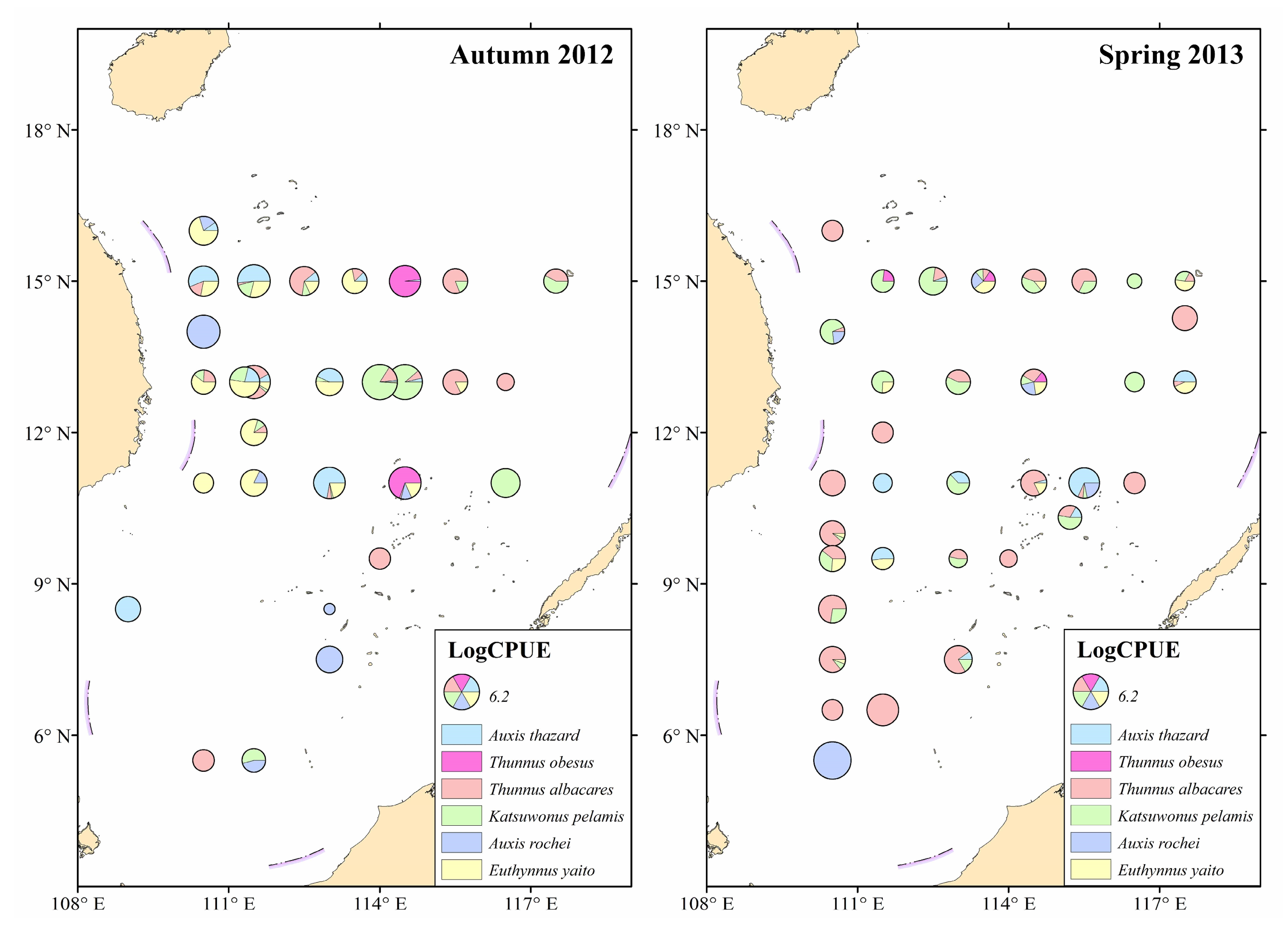
The CPUE for the six juvenile tuna species is shown in Figure 2. They were mainly distributed in the area north of 10° N in autumn 2012, but were more evenly distributed within the survey area in spring 2013.

3.2. Environmental Factors at Study Stations

Histograms showing the values for six environmental factors at study stations where juvenile tuna were present are shown in Figure 3. For those stations the SST ranged from 25.7–29.8 °C (the majority were between 28.5 and 29.5 °C); the ST50 ranged from 19.5–29.3 °C (the majority were between 25 and 29.5 °C); the ST100 ranged from 16.5–24.2 °C (the majority were between 19 and 22 °C); the D50 ranged from −0.3 to 9.8 °C (the majority were between 0 and 6 °C); the D100 ranged from 4.7–12.9 °C (the majority were between 7.5 and 10 °C); and the MLD ranged from 6.8–75.4 m (the majority were between 7 and 24 m).

3.3. Effects of Environmental Factors on the Distribution of Juvenile Tuna Species

Gradient forest analyses were carried out to explore the relationships of the CPUE for juvenile tuna species to all environmental factors investigated. Based on 1000 runs of gradient forests, the mean performance (goodness-of-fit; R f 2 ) for CPUE was 0.183 (sd = 0.013). Of the 1000 runs, the one having the best R2 was used to quantify the relationships between environmental factors and the CPUE of the juvenile tuna species.
The mean importance of predictors (R2), as measured by their contribution to prediction accuracy on the OOB response, was between 0.011 and 0.059 (Figure 4). The D50 was the most important predictor (it had the highest mean importance value: R2 = 0.059), as measured by its contribution to prediction accuracy on the OOB samples, followed by ST50 (R2 = 0.037), MLD (R2 = 0.035), D100 (R2 = 0.020), ST100 (R2 = 0.013), and SST (R2 = 0.011).
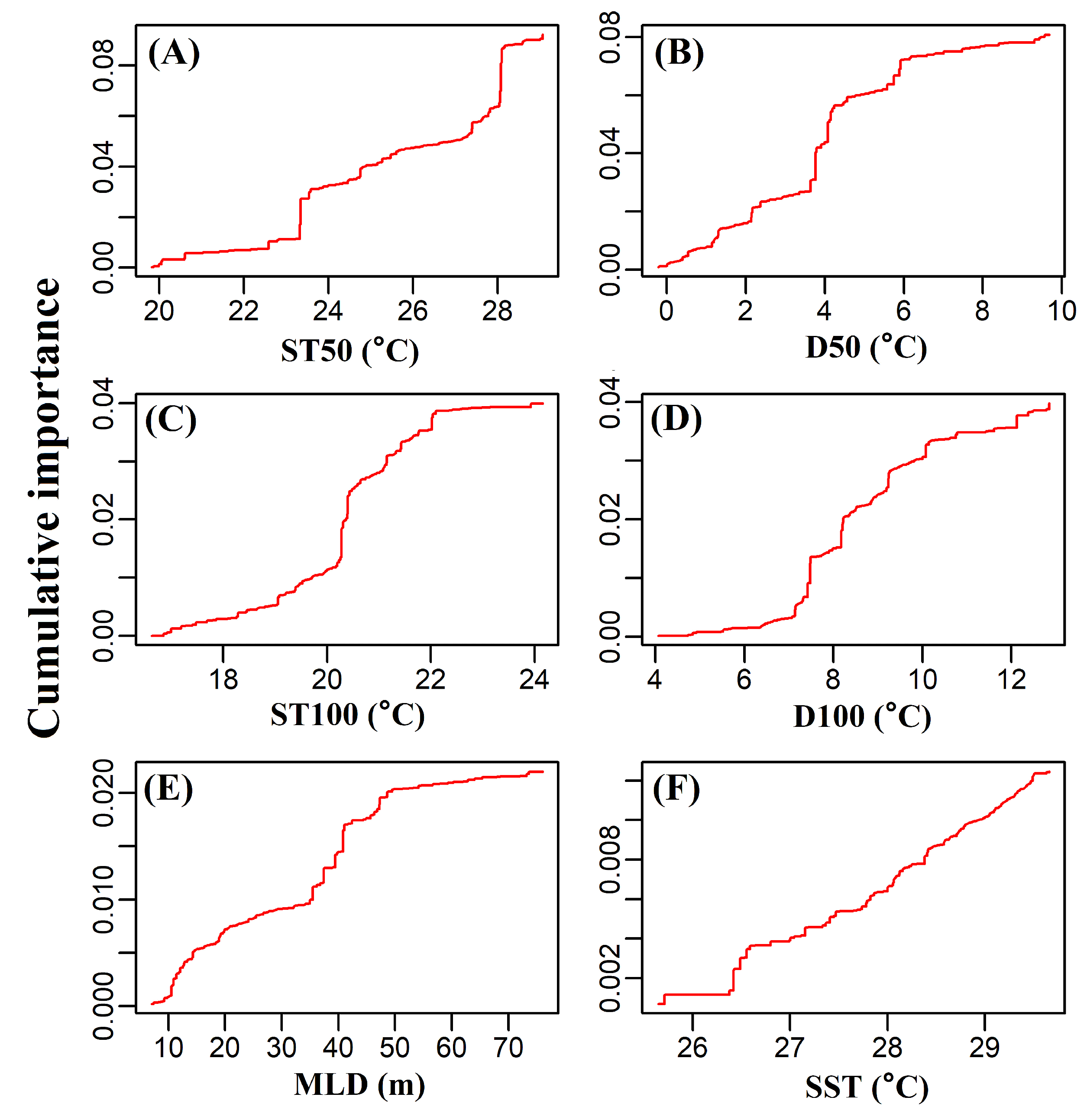
We weighted the CPUE in relation to each of the environmental factors by calculating the cumulative importance distributions of split value improvement scaled by the R2 weighted importance and standardized by the density of observations (Figure 5). The CPUE for juvenile tuna species had a strong threshold response when the values for D50, ST50, the MLD, and SST were approximately 5 °C, 25 °C, 10 m, and 29 °C, respectively.
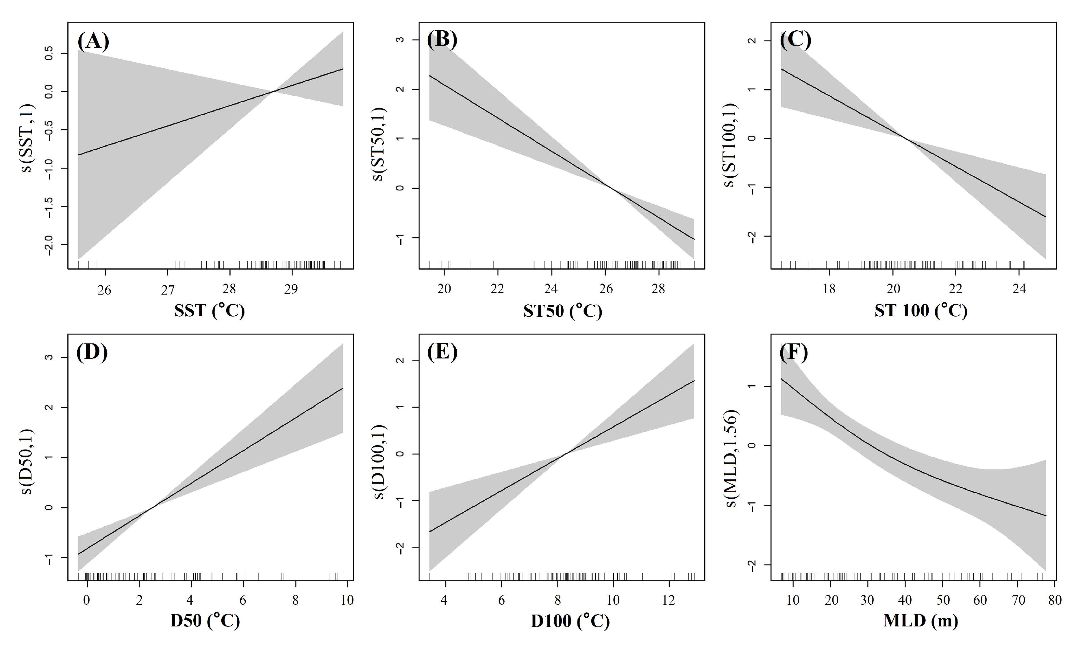
A GAM was used to analyze the individual effects of each predictor variable on the CPUE for juvenile tuna species. The result showed that SST, D50, and D100 were positively related to the CPUE, while ST50, ST100, and the MLD showed negative relationships (Figure 6). These results indicate that higher surface water temperature, lower deep-water temperature, and a shallow MLD were favorable for the aggregation of tuna.

4. Discussion

4.1. Occurrence of Tuna Species in the South China Sea

Tuna species were present at more stations in spring than in the autumn, indicating a wider distribution in spring (Table 1). There are four species of the tuna genus Thunnus in the South China Sea: T. albacares, T. obesus, T. alalonga, and T. thynnus [8,10]. In our surveys the catch of this genus comprised mainly T. albacares with a small amount of T. obesus; T. alalunga and T. thynnus were not caught. A longline fishery survey in 2013 in the South China Sea showed that almost all T. alalunga and T. thynnus were caught in winter, and the catch of T. albacares and T. obesus were much greater in spring and winter than in summer and autumn [8]. Consistent findings imply that the South China Sea is an overwintering ground for T. alalunga and T. thynnus, rather than their long-term habitat. Most catches of T. albacares were juveniles (fork length < 35 cm), which suggests that the South China Sea is the overwintering and spawning ground for T. albacares in winter and spring, with most migrating to the Pacific Ocean for feeding in summer and autumn, and only a small proportion of the population remaining in the South China Sea.

4.2. The Effect of Water Column Temperature on Juvenile Tuna

Sea temperature is generally considered to be the most important environmental factor affecting fish, as it affects the early mortality and growth rate of fish, but is also a major factor driving the seasonal migration of fish and the distribution of fishing grounds [23,43,44]. A study of the relationship between adult T. albacares and SST in the South China Sea by Ji et al. [31] showed that the highest CPUE for juvenile tuna occurred in waters having an SST near 29 °C, and the optimal SST range was empirically determined to be 26.9–29.4 °C. In this study, juvenile tuna species were mainly associated with SSTs between 28.5 and 29.5 °C (Figure 3). However, the gradient forest results showed that SST was the least important among the six environmental factors considered (Figure 4), indicating that the influence of SST on the distribution of juvenile tuna species was not as important as deeper temperature factors in the water column. Among the environmental indices considered in the gradient forest analysis, D50 was significantly more important than the other indices, and the GAM model showed that D50 was positively correlated with the juvenile tuna CPUE (Figure 6), which indicates that a greater temperature difference between the surface layer and the 50 m water layer have also more dense aggregation of juvenile tuna. The GAM analysis also showed a positive relationship between D100 and the CPUE for juvenile tuna species, while ST50, ST100, and MLD showed a negative relationship (Figure 4). These results consistently indicate that the greater the vertical water temperature decrease, the more favorable are the conditions for the aggregation of tuna.
As tuna species can move rapidly through a large range of vertical movements in the water, the temperature of the water column throughout their range of activity can have an effect on them [6]. It has been shown in studies of the Atlantic and Pacific Oceans that vertical water temperature structure is more important than SST in influencing the distribution of tuna [6,13]. Brill et al. [29] suggested that horizontal movements of juvenile bluefin tuna (Thunnus thynnus) are independent of SST in the western North Atlantic, as there is little variation in water temperature compared to vertical temperature. In our study, the difference in SST throughout the survey area was generally <4 °C, while the temperature difference in the deeper layer was greater, up to 10 °C (Figure 3). These data showed similar results that the change in the deep-water temperature was more significant compared with the change in the SST. Lan et al. [13] showed that the depth of the thermocline is inversely proportional to the CPUE in the longline fishery in the West Pacific Ocean, and that a shallow thermocline depth is favorable to the aggregation of fish. Based on tagging data, some studies have showed that free swimming T. albacares are predominantly restricted to depths of the mixed layer, but they occasionally occur below the thermocline for short periods of time [45,46]. These results are similar to our finding on juvenile tuna species that the relationship of the MLD to the juvenile CPUE was inversely proportional. The formation of a shallower mixed layer and large temperature gradients is most likely caused by upwelling, which leads to an increase in primary productivity and consequently improves the potential for predation by tuna species and causes the juvenile tuna to aggregate. Moreover, a shallower mixed layer may have the advantage of resulting in tuna aggregation in the vertical direction, thus facilitating fishing by light falling-net fisheries.
The distribution of oceanic migratory fishes is determined by a combination of marine environmental factors [47]. As tuna are distributed in water depths up to 500 m, the subsurface water column temperature structure has an important influence on fish distribution. In addition to temperature, salinity, complex dynamic oceanic processes, including ocean fronts and eddies, prey and predators, etc., also have an important influence on tuna distribution [11,48]. Salinity is also an important factor, as tuna larvae are more likely to survive in waters with higher salinity. Ocean currents, fronts and eddies can transport larvae to different areas, and they can also affect the availability of food and other resources [48,49]. Juvenile tuna feed on a variety of prey, including small fish, squid, and crustaceans. The availability of these prey items can affect the distribution of tuna larvae, as they are more likely to move to areas with higher prey densities [50]. In addition, the presence of predators can also affect the growth and survival of tuna larvae, as they are more likely to avoid areas with high predator densities.
In this study, both gradient forest analysis and GAM were used to analyze the effect of vertical water column on distribution of juvenile tuna species. The GAM model is generally used to analyze the nonlinear relationship between environmental factors and fisheries. However, the model has an important limitation that there can be no correlation between the environmental factors used in the model simultaneously. However, there is a strong correlation between environmental factors in this study. On the other hand, the gradient forests analysis model can accurately determine the importance of each factor without considering the correlation between environmental factors. By synthesizing the cross-validated R2 and accuracy importance measures from univariate random forest analyses, gradient forest obtains a monotonic function of each predictor that represents the compositional turnover along the gradient of the predictor [39]. It is a regret that the model cannot plot the fitted curves between CPUE and environment factors. Therefore, we used a combination of the two models; the gradient deep forest mainly ranks the importance of the environmental factors, while the GAM model gives the fitted curve of each factor. The results have a good explanation for vertical water column affecting the juvenile tuna species.

5. Conclusions

This study obtained the distribution of six juvenile tuna species (T. albacares, T. obesus, K. pelamis, A. thazard, A. rochei and E. yait) in the South China Sea through light falling-net fishery survey. To analyze the effect of vertical water column on distribution of juvenile tuna species, we used gradient forest and GAM analyze the relationship between environmental factors (SST, ST50, ST100, D50, D100, and MLD) and CPUE of juvenile tuna species. The results of gradient forest analyses showed that D50 was the most important predictor for CPUE with highest mean importance value, followed by ST50, MLD, D100, ST100, and SST. The results of GAM showed that SST, D50, and D100 were positively related to the CPUE, while ST50, ST100, and the MLD showed negative relationships. Our research proved that the subsurface water column temperature structure is more important than SST on the distribution of juvenile tuna species, and relatively rapid vertical decrease in water temperature is favorable for the aggregation of juvenile tuna.

Author Contributions

Conceptualization, S.L., L.L. and P.S.; Data curation, R.Z. and S.C.; Formal analysis, S.L.; Funding acquisition, Y.L. and L.L.; Investigation, S.L., Y.L., X.M., R.Z. and P.S.; Methodology, S.L., R.W. and P.S.; Project administration, L.L.; Resources, L.L.; Software, S.L. and R.W.; Supervision, Y.L., R.W. and X.M.; Validation, Y.L. and X.M.; Visualization, S.L. and S.C.; Writing—original draft, S.L. and Y.L.; Writing—review and editing, L.L. and P.S. All authors have read and agreed to the published version of the manuscript.

Funding

This study was supported by the National Programme on Global Change and Air–Sea Interaction (GASI-01-EIND-YD01/02aut/spr).

Institutional Review Board Statement

The animal study was reviewed and approved by Third Institute of Oceanography, Ministry of Natural Resources.

Data Availability Statement

The datasets generated during and analyzed during the current study are available from the corresponding author on reasonable request.

Conflicts of Interest

The authors declare no conflict of interest.

References

  1. Arrizabalaga, H.; Bruyn, P.; Diaz, G.A.; Murua, H.; Chavance, P.; Molina, A.D.; Gaertner, D.; Ariz, J.; Ruiz, J.; Kell, L.T. Productivity and susceptibility analysis for species caught in Atlantic tuna fisheries. Aquat. Living Resour. 2011, 24, 1–12. [Google Scholar] [CrossRef] [Green Version]
  2. Kaplan, D.M.; Chassot, E.; Amandé, J.M.; Dueri, S.; Demarcq, H.; Dagorn, L.; Fonteneau, A. Spatial management of Indian Ocean tropical tuna fisheries: Potential and perspectives. ICES J. Mar. Sci. 2014, 71, 1728–1749. [Google Scholar] [CrossRef] [Green Version]
  3. Evans, K.; Young, J.W.; Nicol, S.; Kolody, D.; Allain, V.; Bell, J.; Singh, A. Optimising fisheries management in relation to tuna catches in the western central Pacific Ocean: A review of research priorities and opportunities. Mar. Policy 2015, 59, 94–104. [Google Scholar] [CrossRef]
  4. Hallier, J.P.; Gaertner, D. Drifting fish aggregation devices could act as an ecological trap for tropical tuna species. Mar. Ecol. Prog. 2008, 353, 255–264. [Google Scholar] [CrossRef] [Green Version]
  5. Báez, J.C.; Czerwinski, I.A.; Ramos, M.L. Climatic oscillations effect on the yellowfin tuna (Thunnus albacares) Spanish captures in the Indian Ocean. Fish Oceanogr. 2020, 29, 572–583. [Google Scholar] [CrossRef]
  6. Mediodia, H. Effects of sea surface temperature on tuna catch: Evidence from countries in the Eastern Pacific Ocean. Ocean Coast Manag. 2021, 209, 105657. [Google Scholar] [CrossRef]
  7. Lehodey, P.; Senina, I.; Calmettes, B.; Hampton, J.; Nicol, S. Modelling the impact of climate change on pacific skipjack tuna population and fisheries. Clim. Chang. 2013, 119, 95–109. [Google Scholar] [CrossRef]
  8. Feng, B.; Li, Z.; Hou, G. Fish species and quantity in the South China Sea surveyed by deep longline. J. Trop. Oceanogr. 2015, 1, 64–70. [Google Scholar]
  9. Thanh, H. Ocean tuna fishing and marketing in Vietnam. Vietfish 2009, 6, 56–59. [Google Scholar]
  10. Li, Z.; Dong, A.; Wang, M.; Yan, Y.; Lu, H. History and trends of Vietnamese tuna fishery in the South China Sea. J. Modern. Fish Inform. 2014, 1, 60–64. [Google Scholar]
  11. Bakun, A. Ocean eddies, predator pits and bluefin tuna: Implications of an inferred ‘low risk–limited payoff’ reproductive scheme of a (former) archetypical top predator. Fish Fish 2013, 14, 424–438. [Google Scholar] [CrossRef]
  12. Tian, Y.; Uchikawa, K.; Ueda, Y.; Cheng, J. Comparison of fluctuations in fish communities and trophic structures of ecosystems from three currents around Japan: Synchronies and differences. ICES J. Mar. Sci. 2014, 71, 19–34. [Google Scholar] [CrossRef] [Green Version]
  13. Lan, K.W.; Lee, M.A.; Nishida, T.; Lu, H.J.; Weng, J.S.; Chang, Y. Environmental effects on yellowfin tuna catch by the Taiwan longline fishery in the Arabian Sea. Int. J. Remote Sens 2012, 33, 7491–7506. [Google Scholar] [CrossRef]
  14. Ma, S.; Cheng, J.; Li, J.; Liu, Y.; Wan, R.; Tian, Y. Interannual to decadal variability in the catches of small pelagic fishes from China Seas and its responses to climatic regime shifts. Deep-Sea Res II Top Stud. Oceanogr. 2018, 159, 112–129. [Google Scholar] [CrossRef]
  15. Checkley, D.; Alheit, J.; Oozeki, Y.; Roy, C. Climate Change and Small Pelagic Fish. New York, NY, USA, 2009. Available online: https://www.researchgate.net/profile/Juergen-Alheit/publication/266567677_Climate_Change_and_Small_Pelagic_Fish/links/54b5057c0cf26833efd05664/Climate-Change-and-Small-Pelagic-Fish.pdf (accessed on 2 January 2023).
  16. Hollowed, A.B.; Barange, M.; Beamish, R.J.; Brander, K.; Cochrane, K.L.; Drinkwater, K.F.; Foreman, M.G.G.; Hare, J.A.; Holt, J.; Ito, S.-I.; et al. Projected impacts of climate change on marine fish and fisheries. ICES J. Mar. Sci. 2013, 70, 1023–1037. [Google Scholar] [CrossRef] [Green Version]
  17. Pecl, G.T.; Araújo, M.B.; Bell, J.D.; Blanchard, J.; Bonebrake, T.C.; Chen, I.C.; Williams, S.E. Biodiversity redistribution under climate change: Impacts on ecosystems and human well-being. Science 2017, 355, 9214. [Google Scholar] [CrossRef]
  18. Gou, A.; Chen, X. The relationship between ENSO and tuna purse-seine resource abundance and fishing grounds distribution in the Western and Central Pacific Ocean. Mar. Fish 2005, 27, 76–80. [Google Scholar]
  19. Mugo, R.; Saitoh, S.I.; Nihira, A.; Kuroyama, T. Habitat characteristics of skipjack tuna (Katsuwonus pelamis) in the western North Pacific: A remote sensing perspective. Fish Oceanogr. 2010, 19, 382–396. [Google Scholar] [CrossRef]
  20. Lan, K.W.; Lee, M.A.; Lu, H.J.; Shieh, W.J.; Lin, W.K.; Kao, S.C. Ocean variations associated with fishing conditions of yellowfin tuna (Thunnus albacares) in the equatorial Atlantic Ocean. ICES J. Mar. Sci. 2011, 68, 1063–1071. [Google Scholar] [CrossRef]
  21. Lan, K.W.; Evans, K.; Lee, M.A. Effects of climate variability on the distribution and fishing conditions of yellowfin tuna (Thunnus albacares) in the western Indian Ocean. Clim. Chang. 2013, 119, 63–77. [Google Scholar] [CrossRef] [Green Version]
  22. Lan, K.W.; Lee, M.A.; Chou, C.P.; Vayghan, A.H. Association between the interannual variation in the oceanic environment and catch rates of bigeye tuna (Thunnus obesus) in the Atlantic Ocean. Fish Oceanogr. 2018, 27, 395–407. [Google Scholar] [CrossRef]
  23. Kumar, P.S.; Pillai, G.N.; Manjusha, U. El Nino Southern Oscillation (ENSO) impact on tuna fisheries in Indian Ocean. SpringerPlus 2014, 3, 591. [Google Scholar] [CrossRef] [Green Version]
  24. Pikitch, E.; Santora, C.; Babcock, E.; Bakun, A.; Bonfil, R.; Conover, D.; Dayton, P.; Doukakis, P.; Fluharty, D.; Heneman, B. Ecosystem-Based Fishery Management. Policy Forum 2004, 350, 346–347. [Google Scholar] [CrossRef] [PubMed]
  25. Kao, S.-M.; Tseng, H.-S. Scientific Research and Its Influence in Decision-Making of Tuna Regional Fisheries Management Organizations: Case Studies in the Atlantic Ocean and Indian Ocean. Fishes 2022, 7, 76. [Google Scholar] [CrossRef]
  26. Sissenwine, M.P.; Mace, P.M.; Powers, J.E.; Scott, G.P. A commentary on western Atlantic bluefin tuna assessments. Trans. Am. Fish. Soc. 1998, 127, 838–855. [Google Scholar] [CrossRef]
  27. Liu, S.; Liu, Y.; Fu, C.; Yan, L.; Xu, Y.; Wan, R.; Li, J.; Tian, Y. Using novel spawning ground indices to analyze the effects of climate change on Pacifc saury abundance. J. Mar. Syst. 2019, 191, 13–23. [Google Scholar] [CrossRef]
  28. Wiryawan, B.; Loneragan, N.; Mardhiah, U.; Kleinertz, S.; Wahyuningrum, P.I.; Pingkan, J.; Wildan, T.; Duggan, D.; Yulianto, I. Catch per Unit Effort Dynamic of Yellowfin Tuna Related to Sea Surface Temperature and Chlorophyll in Southern Indonesia. Fishes 2020, 5, 28. [Google Scholar] [CrossRef]
  29. Brill, R.; Lutcavage, R.; Metzger, G.; Bushnell, P.; Lucy, M.; Foley, D. Horizontal and vertical movements of juvenile bluefin tuna (Thunnus thynnus), in relation to oceanographic conditions of the western North Atlantic, determined with ultrasonic telemetry. Fish Bull 2021, 100, 155–167. [Google Scholar]
  30. Blank, J.M.; Morrissette, J.M.; Farwell, C.J.; Price, M.; Schallert, R.J.; Block, B.A. Temperature effects on metabolic rate of juvenile Pacific bluefin tuna Thunnus orientalis. J. Exp. Biol. 2007, 210, 4254–4261. [Google Scholar] [CrossRef] [Green Version]
  31. Ji, S.; Zhou, W.; Xu, H.; Wang, X. A WebGIS application: Tuna fishing ground forecasting information service system for the open South China Sea. In Proceedings of the 2016 IEEE International Geoscience and Remote Sensing Symposium, Beijing, China, 10–15 July 2016; pp. 3628–3631. [Google Scholar]
  32. Zhou, W.; Li, A.; Ji, S.; Qiu, Y. Yellowfin Tuna (Thunnusalbacares) Fishing Ground Forecasting Model Based on Bayes Classifier in The South China Sea. Pol. Marit. Res. 2017, 24, 140–146. [Google Scholar] [CrossRef] [Green Version]
  33. Arrizabalaga, H.; Pereira, J.G.; Royer, F.; Galuardi, B.; Goni, N.; Artetxe, I.; Lutcavage, M. Bigeye tuna (Thunnus obesus) vertical movements in the Azores Islands determined with pop-up satellite archival tags. Fish Oceanogr. 2008, 17, 74–83. [Google Scholar] [CrossRef]
  34. Williams, A.J.; Allain, V.; Nicol, S.J.; Evans, K.J.; Hoyle, S.D.; Dupoux, C.; Vourey, E.; Dubosc, J. Vertical behavior and diet of albacore tuna (Thunnus alalunga) vary with latitude in the South Pacific Ocean. Deep-Sea Res. II Top Stud. Oceanogr. 2015, 113, 154–169. [Google Scholar] [CrossRef]
  35. Uchiyama, J.; Struhsaker, P. Age and growth of skipjack tuna, Katsuwonus pelamis, and yellowfin tuna, Thunnus albacares, as indicated by daily growth increments of sagittae. Fish Bull. 1981, 79, 151–162. [Google Scholar]
  36. Neilson, J.D.; Campana, S.E. A validated description of age and growth of western Atlantic bluefin tuna (Thunnus thynnus). Can. J. Fish Aquat. Sci. 2008, 65, 1523–1527. [Google Scholar] [CrossRef]
  37. Soares, J.B.; Monteiro-Neto, C.; Costa, M.R.D.; Martins, R.R.M.; Vieira, F.C.D.S.; Andrade-Tubino, M.F.D.; Bastos, A.L.; Tubino, R.D.A. Size structure, reproduction, and growth of skipjack tuna (Katsuwonus pelamis) caught by the pole-and-line fleet in the southwest Atlantic. Fish Res. 2019, 212, 136–145. [Google Scholar] [CrossRef]
  38. Shi, P.; Du, Y.; Wang, D.; Gan, Z. Annual cycle of mixed layer in South China Sea. J. Trop Oceanogr. 2001, 20, 10–17. [Google Scholar]
  39. Ellis, N.; Smith, S.J.; Pitcher, C.R. Gradient forests: Calculating importance gradients on physical predictors. Ecology 2012, 93, 156–168. [Google Scholar] [CrossRef]
  40. Hastie, T.J.; Tibshirani, R.J. Generalized Additive Models. Stat Sci. 1986, 1, 297–310. [Google Scholar] [CrossRef]
  41. Litzow, M.A.; Hobday, A.J.; Frusher, S.D.; Dann, P.; Tuck, G.N. Detecting regime shifts in marine systems with limited biological data: An example from southeast Australia. Prog. Oceanogr. 2016, 14, 96–108. [Google Scholar] [CrossRef]
  42. Pang, Y.; Tian, Y.; Fu, C.; Wang, B.; Li, J.; Ren, Y.; Wan, R. Variability of coastal cephalopods in overexploited China Seas under climate change with implications on fisheries management. Fish Res. 2018, 208, 22–33. [Google Scholar] [CrossRef]
  43. Tittensor, D.P.; Mora, C.; Jetz, W.; Lotze, H.K.; Ricard, D.; Berghe, E.V.; Worm, B. Global patterns and predictors of marine biodiversity across taxa. Nature 2010, 466, 1098–1101. [Google Scholar] [CrossRef] [PubMed]
  44. Tseng, C.T.; Sun, C.L.; Belkin, I.M.; Yeh, S.Z.; Kuo, C.L.; Liu, D.C. Sea surface temperature fronts affect distribution of Pacific saury (Cololabis saira) in the Northwestern Pacific Ocean. Deep-Sea Res II Top Stud Oceanogr. 2014, 107, 15–21. [Google Scholar] [CrossRef]
  45. Dagorn, L.; Holland, K.N.; Hallier, J.-P.; Taquet, M.; Moreno, G.; Sancho, G.; Itano, D.G.; Aumeeruddy, R.; Girard, C.; Million, J.; et al. Deep diving behavior observed in yellowfin tuna (Thunnus albacares). Aquat. Living Res. 2006, 19, 85–88. [Google Scholar] [CrossRef] [Green Version]
  46. Schaefer, K.M.; Fuller, D.W. Movements, behavior, and habitat utilization of yellowfin tuna (Thunnus albacares) in the northeastern Pacific Ocean, ascertained through archival tag data. Mar. Biol. 2007, 152, 503–525. [Google Scholar] [CrossRef]
  47. Zainuddin, M.; Saitoh, K.; Saitoh, S.I. Albacore (Thunnus alalunga) fishing ground in relation to oceanographic conditions in the western North Pacific Ocean using remotely sensed satellite data. Fish Oceanogr. 2008, 17, 61–73. [Google Scholar] [CrossRef] [Green Version]
  48. Syah, A.F.; Saitoh, S.I.; Alabia, I.D.; Hirawake, T. Detection of potential fishing zone for Pacific saury (Cololabis saira) using generalized additive model and remotely sensed data. IOP Conf. Ser. Earth Env. Sci. 2017, 54, 012074. [Google Scholar] [CrossRef]
  49. Kuroda, H.; Yokouchi, K. Interdecadal decrease in potential fishing areas for Pacific saury off the southeastern coast of Hokkaido, Japan. Fish. Oceanogr. 2017, 26, 439–454. [Google Scholar] [CrossRef]
  50. Bakun, A. Fronts and eddies as key structures in the habitat of marine fish larvae: Opportunity, adaptive response and competitive advantage. Sci. Mar. 2006, 70, 105–122. [Google Scholar] [CrossRef]
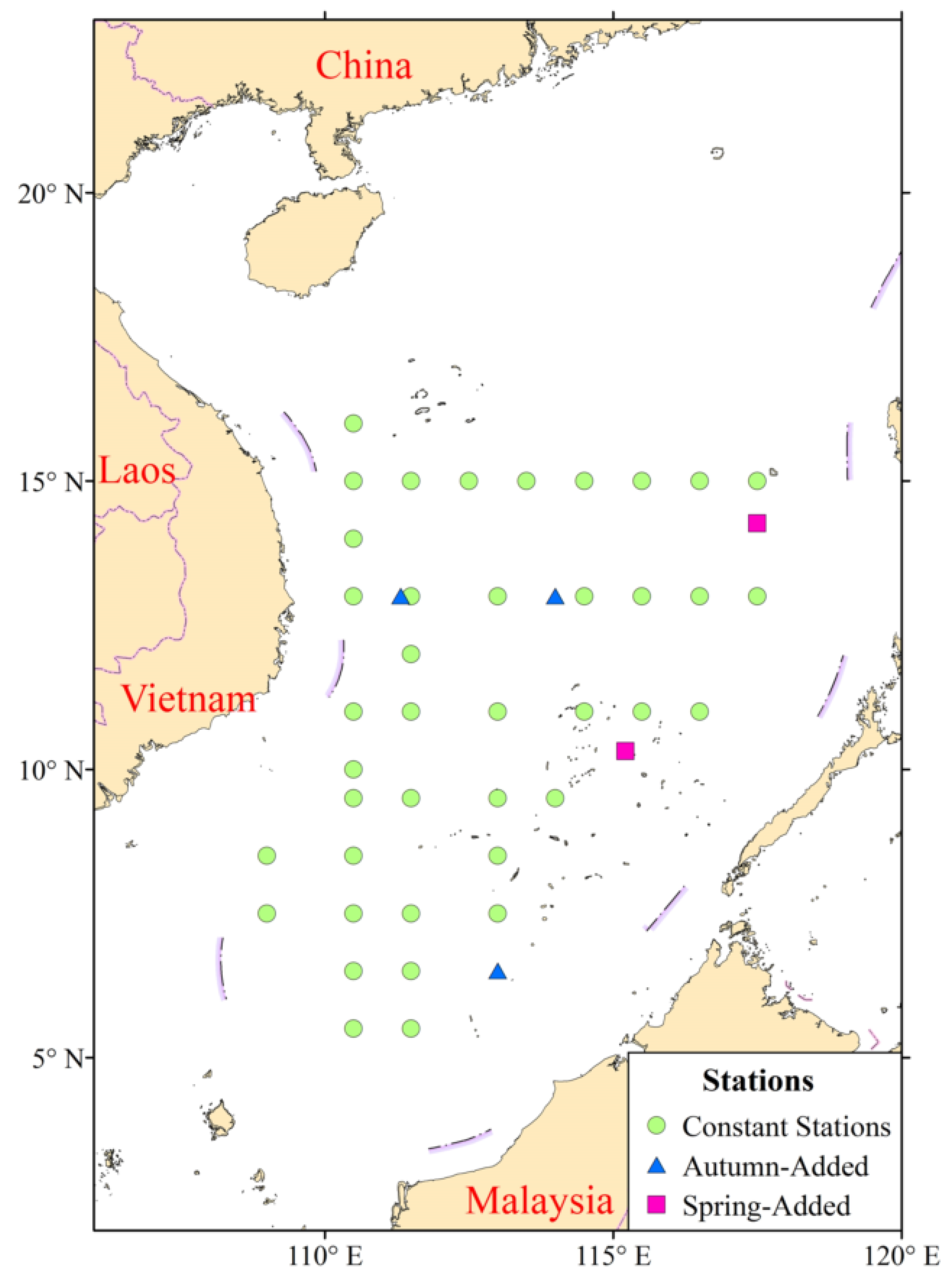
Figure 1. Distribution of stations for surveys in autumn 2012 and spring 2013. Green circles indicate stations common to both surveys; blue triangles represent additional stations in autumn 2012; pink squares represent additional stations in spring 2013.
Fishes 08 00135 g001
Figure 2. CPUE distribution for six juvenile tuna species (T. albacares, T. obesus, K. pelamis, A. thazard, A. rochei, and E. yaito).
Fishes 08 00135 g002
Figure 3. Data for six environmental factors: (A) SST, (B) ST50, (C) ST100, (D) D50, (E) D100, and (F) MLD for stations at which juvenile tuna species were present.
Fishes 08 00135 g003
Figure 4. Importance of environmental variables: ST50, D50, ST100, D100, MLD, and SST across CPUE outputs (R2) from the gradient forest analyses.
Fishes 08 00135 g004
Figure 5. Cumulative shifts (in R2 units) of the CPUE for juvenile tuna species in response to environmental variables: (A) ST50, (B) D50, (C) ST100, (D) D100, (E) MLD, and (F) SST.
Fishes 08 00135 g005
Figure 6. GAM-derived effect of environmental factors on CPUE of juvenile tuna species, based on the model constructed using: (A) SST, (B) ST50, (C) ST100, (D) D50, (E) D100, and (F) MLD. Rug plots on the horizontal axis represent observed data points, and the fitted function is shown by the solid line. The gray shading shows the 95% confidence interval.
Fishes 08 00135 g006
Table 1. Juvenile tuna species capture information.
SpeciesAutumn 2012Spring 2013
Number of Present StationsTotal Catch (kg)Number of Present StationsTotal Catch (kg)
T. albacares19446.8226103.03
T. obesus2145.0030.40
K. pelamis161810.802212.95
A. thazard13245.951026.79
A. rochei8223.1356474.20
E. yaito19174.84122.27
Tuna species293046.53346619.63
Disclaimer/Publisher’s Note: The statements, opinions and data contained in all publications are solely those of the individual author(s) and contributor(s) and not of MDPI and/or the editor(s). MDPI and/or the editor(s) disclaim responsibility for any injury to people or property resulting from any ideas, methods, instructions or products referred to in the content.