Abstract
Pacific sardine (Sardinops sagax) is a commercially important species and supports important fisheries in the Northwest Pacific Ocean (NPO). Understanding the habitat distribution patterns of Pacific sardine is of great significance for fishing ground prediction and stock management. In this study, both single-algorithm and ensemble distribution models were established through the Biomod2 package for Pacific sardine by combining the species occurrence data, sea surface temperature (SST), sea surface height (SSH), sea surface salinity (SSS) and chlorophyll-a concentration (Chla) in the NPO during the main fishing season (June–November) from 2015 to 2020. The results indicated that the key environmental variables affecting the habitat distribution of Pacific sardine were the SSH and SST. The suitable habitat area for Pacific sardine showed significant monthly changes: the suitable habitat range in June was larger than that in July and August, while the suitable habitat range gradually increased from September to November. Furthermore, the monthly geometric centers of habitat suitability index (HSI) for Pacific sardine presented a counterclockwise pattern, gradually moving to the northeast from June, and then turning back to the southwest from August. Compared with single-algorithm models, the ensemble model had higher evaluation metric values and better spatial correspondence between habitat prediction and occurrence records data, which indicated that the ensemble model can provide more accurate prediction and is a promising tool for potential habitat forecasting and resource management.
1. Introduction
Fishery resources are the foundation for the development of fisheries and related industries, and are one of the main sources of high-quality protein for humans [1]. Marine environmental changes can have direct or indirect influences on the marine ecosystems that have consequences for the spatio-temporal distribution, resource abundance and productivity of marine species, as well as their interactions with each other [2,3,4]. Marine species, in turn, are predicted to respond to environmental variations in suitable distribution areas through genetic adaptation or changing distribution ranges [5,6]. Therefore, understanding the suitable habitat distribution and the dynamics of habitat distribution under environmental change is of great significance to the sustainable use and management of fisheries resources.
Pacific sardine (Sardinops sagax) is widely distributed in the warm temperate waters of the Indo-Pacific and is also one of the most important pelagic stocks in the Northwest Pacific Ocean (NPO) [7,8,9]. Pacific sardine can reach a maximum age of 6–7 years [10,11], and attain sexual maturity at two years old, with an average length at maturity (L50) of 180 mm and an average weight higher or equal to 180 g [12]. The gonadosomatic index of female Pacific sardine varies depending on the area, with maximum values at 11 °C water temperature [13,14]. The main spawning time of Pacific sardine has been reported to be from February to March along central and southern Japan [15]. Sardine larvae are transported to the northeast by the Kuroshio and Kuroshio Extension, then continued to migrate to the northeast, reaching the feeding grounds in summer [16]. In winter, Pacific sardine migrate southwest along the Pacific coast of southern Japan to spawning grounds [17]. Japanese fishermen were pioneers in exploiting this species in the 1920s, and China began a fishery for these resources in the 1980s [18]. At present, Pacific sardine is mainly exploited by Japan, China (including Chinese Taipei) and Korea. The annual catch of Pacific sardine recorded in 2019 in China was about 24,773 tons, which accounted for 11.1% of global production [19]. Moreover, the proportion of Pacific sardine catches in the NPO of China showed a gradually increasing trend from 2014 to 2020 [20]. Due to their increasing ecological and economic value, the utilization and management of Pacific sardine resources have raised widespread concern and these fish have been listed among the priority fish species by the North Pacific Fisheries Commission (NPFC) [21].
Owing to the short life cycle and long migration route of Pacific sardine, large-scale climate events and regional environmental changes are generally considered to be important factors that affect the Pacific sardine population [22,23]. Many studies indicated that like other small pelagic species, the habitat distribution of Pacific sardine is largely influenced by marine environmental factors, such as the sea surface temperature (SST), sea surface height (SSH), chlorophyll-a concentration (Chla) and sea surface salinity (SSS) [24,25,26]. For instance, Dudarev [27] indicated that 8–20 °C and 15–30 m are the suitable SST and depth for the Pacific sardine distribution in the NPO, respectively. Vander et al. [28] studied the effects of the SST, SSS and SSH on the distribution of Pacific sardine and the results showed that the SST has a higher impact than the SSH and SSS. Takasuka et al. [29] put forward a simple “optimal growth temperature” hypothesis and investigated the relationship between the growth rate of Pacific sardine and SST. The results showed dome-shaped relationships between the growth rate and SST, with the optimal growth rate occurring when the temperature was 16.2 °C. To our knowledge, there are few studies that investigated the spatial variation in the potential habitat distribution of Pacific sardine.
A species distribution model (SDM) is widely considered a significant tool for predicting a species’ potential distribution and the influence of climate change on its distribution, which can combine the species occurrence data and environmental variables [30,31]. SDMs were successfully used to predict the potential distribution of many species. For instance, Gong et al. [32] applied maximum entropy (MaxEnt) to forecast the potential distribution of neon flying squid and projected potential habitat ranges under future climate scenarios. Guénard et al. [33] used a deep feed-forward artificial neural network (ANN) to model habitat suitability for Lake sturgeon (Acipenser fulvescens) and White perch (Morone americana). MaxEnt was used by Zhang et al. [34] to study the influencing mechanism of marine environmental factors on the potential fishing grounds for Pacific saury (Cololabis saira) in the NPO, and the distribution range shifts in different months of potential distribution were revealed. With the development of computer technology and modeling algorithms, dozens of SDMs were proposed to meet the increasing demand for potential habitat prediction and fishing grounds searches for marine species [35]. However, the statistical and predictive performances of different models are varied, which are attributed to the differences in their scope of application and theoretical algorithms. MaxEnt is one of the most frequently used SDMs and is generally considered to have a good evaluation performance [36,37]; it is also simple to operate, easy to use and can deal with high-capacity data [38]. Thuiller [39] indicated that the performance of SDM decreases with the increase of input data, and it is not stable and reliable to use only a certain model for potential distribution prediction. The Biomod modeling package can integrate the results of multiple models and use the comprehensive results as the output of the ensemble model to improve the accuracy of prediction results [40]. The latest version is Biomod2, which was updated in 2016. Biomod2 has been widely recognized and used for the potential distribution prediction of many species since its publication [41,42,43].
To reasonably utilize and manage Pacific sardine resources in the NPO, it is important to understand their potential habitat distribution and the impact of the environment on habitat suitability. However, previous research on the Pacific sardine in this area mainly focused on basic biology, and there was little research on suitable habitat prediction [44,45]. In addition, challenges and uncertainties still exist in the research to predict the suitable habitat distribution of Pacific sardine in the NPO. Thus, Biomod2 was applied in this study to investigate the potential distribution of Pacific sardine in the NPO. The predictive performance of the single-algorithm model and ensemble model in the Biomod2 package was tested. The main objectives of this study were (1) to determine the key environmental variables influencing the habitat distribution of Pacific sardine, (2) to identify the monthly habitat patterns of Pacific sardine in the main fishing seasons (June to November), and (3) to compare the predictive performances of single algorithm model and ensemble model and explore their application prospects.
2. Materials and Methods
2.1. Study Area
In this research, the study area was distributed between 38–45° N and 145–160° E, covering the main fishing grounds of Pacific sardine in the NPO (Figure 1). This area is situated at the junction of the Kuroshio warm current and the Oyashio cold current, which is one of the high-yield sea areas around the world. Many economically important fish species, such as tunas (Thunnus spp.), Pacific saury (Cololabis saira), Chub mackerel (Scomber japonicas) and Pacific sardine, inhabit this zone.
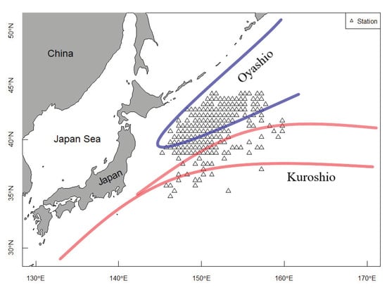
Figure 1.
Location of fishing grounds for Pacific sardine in the NPO. The Oyashio cold current is represented using the blue lines and the Kuroshio warm current is shown using the red lines.
2.2. Data Resources
Species occurrence data and environmental variables are essential inputs for ecological niche models and SDMs. Both inputs are used to detect potentially habitable sites of target species in the study area [46]. In this study, occurrence data with a spatial resolution grid of 0.25° latitude × 0.25° longitude of Pacific sardine was derived from the Technical Group for Trawl-Purse Seine Fishery, Distant-Water Fishery Society of China, covering the period between June and November from 2015 to 2020. In total, 599 occurrence records of Pacific sardine were included in this study, and the number of occurrence records in each month is shown in Table 1. Environmental variables that predominantly influence the abundance and distribution of Pacific sardine stock, including SST, SSH, SSS and Chla, were selected for species distribution modeling given that they were reported in the literature as important variables that influence the abundance and distribution of Pacific sardine stock [47]. Those data were downloaded from the Copernicus Marine Service (http://marine.copernicus.eu, accessed on 23 May 2022). In order to match with the spatio-temporal resolution of the species occurrence data, all the environmental data were downloaded at 0.25° spatial resolution and monthly temporal resolution.

Table 1.
The number of occurrence records of the Pacific sardine by month from 2015 to 2020.
In order to ensure that the multicollinearity of environmental variables did not affect the predictive ability and lead to overfitting [48], the mutual independence of environmental variables was checked by the variance inflation factor (VIF) (Table 2). The VIF values of the environmental variables were less than 3, except for the SSS. However, the VIF of the SSS was less than 10, indicating that there was no serious multi-collinearity among the environmental variables [49,50].
Table 2.
Variance inflation factors (VIFs) of the environmental variables.
2.3. Modelling Procedure
The Biomod2 package in the R(V4.0.2) environment was used to predict the potential distribution of Pacific sardine in this study, which included ten models: generalized linear model (GLM), generalized additive model (GAM), multiple adaptive regression splines (MARS), generalized boosting model (GBM), classification tree analysis (CTA), ANN, surface range envelope (SRE), flexible discriminant analysis (FDA), random forest (RF) and MaxEnt. During the modeling process, the first step was to construct the single-algorithm Pacific sardine habitat model. Three groups of pseudoabsence records were randomly generated based on the occurrence data and background data of the Pacific sardine, and each group had 500 pseudoabsence records [46]. In order to evaluate the accuracy of the model, we randomly selected 70% of the occurrence data as the training dataset and the remaining 30% as the validation dataset, and the weight of occurrence points was equal to pseudoabsence points when the model was running and evaluating [51]. Each model was run ten times, with a total of 1800 single-algorithm model results (3 groups of pseudoabsence records × running 10 times × 10 single-algorithm models × 6 months). The true skill statistic (TSS), Cohen’s kappa statistic (Kappa) and the area under the receiver operating characteristic curve (AUC) were applied as evaluation metrics to assess the performance of the models [52,53]. The measurement standards for TSS, Kappa and AUC are shown in Table 3, and the closer each of their values was to 1, the more reliable the prediction results were [54]. Furthermore, the relative importance of environmental variables was calculated in order to better understand the environmental factors that affected the habitat of the Pacific sardine in the NPO.
Table 3.
Measurement standard for TSS, Kappa and AUC.
The second step was to develop the ensemble model. In order to reduce the uncertainty of the single-algorithm model and data generation process (mainly pseudoabsence sites), we formulated the ensemble species distribution model to predict the spatial distribution of suitable habitats for the Pacific sardine in the NPO. In this study, individual models with AUC ≥ 0.9, TSS ≥ 0.7 and Kappa ≥ 0.6 were kept to construct the ensemble species distribution model of the Pacific sardine based on a range of published work [55,56]. A total of 6 ensemble models were constructed in this study, that is, one per month from June to November. The potential suitable habitat distribution results of the Pacific sardine based on the ensemble model were normalized, and the habitat distribution map of the Pacific sardine was made using ArcGIS 10.3. The grid value in the map represents the probability of species occurrence in the fishing area, and the habitat suitability index (HSI) ranges from 0 to 1, where the closer the grid value is to 1, the higher the probability of species occurrence. According to the results by Chen et al. [57] and Yu et al. [58], the areas with HIS ≥ 0.6, with 0.2 < HIS < 0.6 and with HIS ≤ 0.2 were defined as a suitable habitat, a common habitat and a poor habitat, respectively, for the Pacific sardine stock in the NPO.
2.4. Centroid Shifts
To show the change in the spatial distribution of the suitable habitat due to environmental variation, monthly longitudinal geometric centers of the HSI (LONGHSI) and latitudinal geometric centers of the HSI (LATGHSI) were calculated. The LONGHSI and LATGHSI were determined using the following equations [59]:
where Longitude(i,m) and Latitude(i,m) were the longitude and latitude of the ith fishing unit in month m, respectively. HSI(i,m) is the HSI value within the ith fishing unit in month m.
3. Results
3.1. Single-Algorithm Models Performances
The TSS, Kappa and AUC values of all ten single-algorithm models for each month were calculated based on the cross-validation evaluation (Table 4). The evaluation results revealed that different optimal models could be obtained for different months using different evaluation metrics. For instance, in June, MaxEnt was the optimal model under the three evaluation metrics. For July, the GAM model was the optimal model based on the TSS values, the RF model was the optimal model based on the Kappa values and the MaxEnt model was the best model based on the AUC values. Furthermore, for November, the MaxEnt model had the highest Kappa and AUC values, whereas the MARS model had the largest TSS value. The above results showed the uncertainty of statistical precision of single-algorithm models. Considering the AUC performance metrics, the models with the best predictive performance from June to November were all MaxEnt models (0.938, 0.975, 0.910, 0.911, 0.929 and 0.946, respectively), and the worst ones were all SRE models (0.839, 0.872, 0.737, 0.764, 0.817 and 0.852, respectively) (Table 4).
Table 4.
Evaluation metrics for single-algorithm models.
The averaged relative environmental variable importance of each single-algorithm model is shown in Figure 2. The analysis pointed out that the SSH was the most important environmental variable affecting the habitat distribution of the Pacific sardine in the NPO in all single-algorithm models, except for the SRE model, followed by the SST. In the SRE model, the SST and Chla were the two most significant environmental variables, which contributed 39.0% and 36.6% to the model, respectively, followed by the SSS (34.3%) and SSH (30.7%). For the single-algorithm models, in most cases, the MaxEnt model was the optimal model, and if selected based on the AUC evaluation metric, MaxEnt was the best model for every month (Table 4). Therefore, the monthly averaged predicted potential habitat distribution of the Pacific sardine in the NPO predicted using MaxEnt model is shown in Figure 3. The distribution range of the suitable habitat for the Pacific sardine varied between months. The suitable habitat area showed a fluctuating trend (first decreasing and then increasing) from June to November, and the corresponding proportion of pixels with a probability higher than or equal to 0.6 was June (6.4%), July (4.8%), August (4.2%), September (6.7%), October (7.5%) and November (8.4%). While most of the occurrences coincided with suitable habitat areas (HIS ≥ 0.6), there were some that appeared in a common habitat (0.2 < HIS < 0.6) or a poor habitat (HIS ≤ 0.2) (Figure 3).
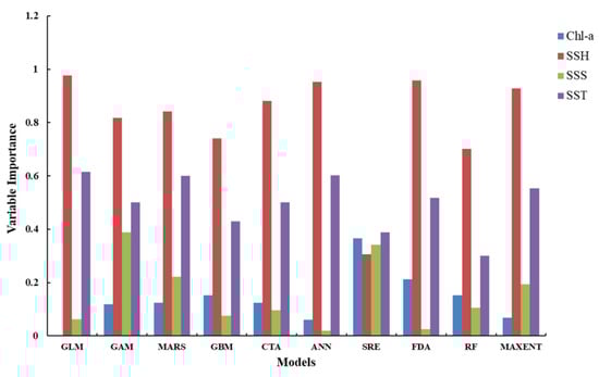
Figure 2.
Relative environmental variable importance derived from the single-algorithm models.
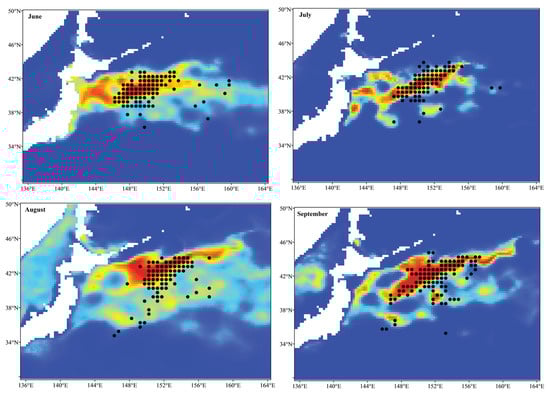
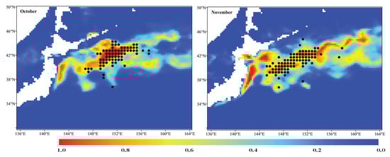
Figure 3.
Predicted potential habitat distribution of the Pacific sardine in the NPO using the top single-algorithm model (MaxEnt) with the highest AUC value between June and November from 2015 to 2020. The black points represent the operation positions of the Pacific sardine fishing grounds.
3.2. Ensemble Model Prediction and Potential Habitat Distribution of the Pacific Sardine
Table 5 shows the model compositions and evaluation metric values of the ensemble models from June to November. The three evaluation metrics of the ensemble models from June to November were all higher than the corresponding single-algorithm models, which revealed that the ensemble models provided more robust predictions (Table 4, Table 5). The environmental variables permutation importance of the ensemble models for different months was shown in Figure 4, indicating that the SSH and SST played the most important roles in the potential distribution of the Pacific sardine, and their mean contribution rates were 68.3% and 46.3%, respectively. In relative terms, the Chla and SSS contributed little to the predictive performance of the model, which was consistent with the results of the single-algorithm models in Figure 2.
Table 5.
Evaluation metrics and model compositions for the ensemble models.
Figure 4.
Permutation importance of the environmental variables for different months.
Figure 5 exhibits the monthly averaged potential habitats of the Pacific sardine for the ensemble models between June and November from 2015 to 2020. In June, the Pacific sardine suitable habitats (HIS ≥ 0.6) mainly occurred in the waters between 36–42° N and 145–160° E of NPO. The suitable Pacific sardine habitat areas of July and August were narrow in extent and shifted from south to north from June to August. Suitable habitat areas in September were larger than those in July and August, and the areas appeared to be larger and shifted from north to south from September to November. Moreover, the habitat prediction maps for September to November revealed that the fishing vessels of Pacific sardine were mainly concentrated in suitable habitat areas, and the spatial correspondence between the habitat predictions and occurrence records data of the ensemble model was better than the single-algorithm models (Figure 3, Figure 5). Figure 6 reveals the monthly SST, SSH, Chla and SSS values for the fishing grounds of the Pacific sardine fishery from 2015 to 2020. The SST increased first and then decreased with the increase in months, while the Chla showed the opposite trend. The SSH increased gradually with the increase in months, while the SSS was relatively stable (Figure 6).
Figure 5.
Distribution of the Pacific sardine potential habitats simulated using the ensemble models between June and November from 2015 to 2020 in the NPO. The black points represent the operation positions of the Pacific sardine fishing grounds.
Figure 6.
Monthly satellite-based (A) SST, (B) SSH, (C) Chla and (D) SSS values for the fishing grounds of the Pacific sardine fishery between 2015 and 2020.
3.3. Centroid Shifts of Pacific Sardine Fishing Grounds
Variation in the geometric centers of the HSI between June and November during 2015–2020 is shown in Figure 7. It can be seen from the figure that the geometric centers of the HSI for the Pacific sardine presented a counterclockwise pattern, gradually moving to the northeast from June, reaching the northeast end in August, and then turning back to the southwest from September, which pointed out that the geometric center of the HSI had obvious seasonal changes. The variation range of the longitude and latitude of the HSI geometric center was between 41°6′ and 42°22′ N and between 149°51′ and 152°14′ E (Figure 7).
Figure 7.
Variation of the geometric centers of the HSI between June and November from 2015 to 2020.
4. Discussion
SDMs, such as GAM, ANN and MaxEnt, have been widely used to predict suitable habitats, map habitat variations and evaluate the relationship between species distribution and the marine environment [60,61,62]. Monthly suitable habitat distributions of the Pacific sardine in the NPO were predicted in this study based on Biomod2 combined with species occurrence data and environmental variables. There were some issues with the Biomod2 applied in this study that need to be explained here. First, compared with a single-algorithm model, such as MaxEnt and GAM, Biomod2 can map the overall variation of all models and can integrate other aspects of different models, such as the variable importance or model response curves [41]. Therefore, Biomod2 was used in this study to predict the habitat distribution of the Pacific sardine. Second, the data series used in this research included just six years (2015–2020). The reason for this was that the Pacific sardine fishery in the NPO of China started relatively late and the data was limited, which may have affected the results of the model. The sensitivity analysis of this data series will be carried out in future research. Finally, our research was one of the few examples that predicted the monthly habitat variation pattern of the Pacific sardine in the NPO using the ensemble model based on Biomod2, which could provide accurate information for the sustainable utilization and conservation of this species.
Figure 2 indicated that while the relative importance rankings of environmental variables for the single-algorithm models were fairly consistent, the statistical performance differed between the models (Table 4), which revealed that the inherent differences and uncertainties between the individual models and the prediction performance varied widely [36]. The monthly TSS, Kappa and AUC values in the ensemble model were all higher than the corresponding monthly values in the single-algorithm model (Table 4, Table 5). In addition, the species occurrence points of the ensemble model were mainly concentrated in high-HSI areas, and the predicted habitat had a better spatial correspondence with reality relative to the top-performing single-algorithm models (Figure 3, Figure 5). The above conclusions reinforced the findings of previous studies showing that the ensemble model is more robust than the single-algorithm models in predicting suitable habitats for marine organisms [63,64,65]. Therefore, the ensemble model is expected to become an important tool for fishing grounds forecasting and resource management.
Figure 2 and Figure 4 showed the relative importance of environmental variables for the single-algorithm models and the ensemble model, respectively, which demonstrated that the SSH and SST contributed more to the Pacific sardine habitat model than the Chla and SSS, and were important environmental factors that affected the Pacific sardine habitat distribution. Arkhipkin et al. [66] reported that although environmental factors, such as the SSS, play an important role in the population dynamics of pelagic species, their contributions are relatively small compared to the SSH and SST, which is consistent with the results of this study. Moreover, the findings in this study underpinned the importance of the SSH and SST in the habitat distributions of the Pacific sardine in the NPO. Pacific sardine is a small warm-temperate pelagic stock, which is sensitive to the SST in their habitat area. At the same time, plankton is the main prey of Pacific sardine, and the SSH can change the spatial distribution of this food concentration, which is why the SSH and SST have a greater impact on the habitat distribution of Pacific sardine.
Figure 5 showed that the suitable habitats for the Pacific sardine were mainly distributed between 38° and 43° N and between 145° and 156° E. However, the habitat patterns of Pacific sardine in the NPO exhibited significant monthly variations from June to November. The spatial pattern of suitable habitats was closely related to the changes in the marine environment in the NPO. The area of suitable habitat for the Pacific sardine gradually decreased from June to August and increased from September to November (Figure 5). Correspondingly, the SST increased from 15.19 °C in June to 22.10 °C in August, and then gradually decreased, and the SST decreased to 14.25 °C in November. Therefore, it was preliminarily determined that the optimal SST for sardine fishing grounds was approximately 13 °C to 15 °C (Figure 6A), which was consistent with previous studies [67]. The SSH could indicate the mesoscale activity in the NPO. Convergence drives the local food concentration into different spatial patterns, and it is a physical driver of small pelagic species distribution [68]. In this study, as the environmental variable with the highest contribution rate (Figure 2, Figure 4), the SSH gradually increased from June to October, and then decreased, and the overall change in the SSH value was small (Figure 6B). However, there was no regular correspondence with the area changes of suitable habitats, which may have been related to the complicated mechanism of the SSH affecting the distribution of Pacific sardine habitats [69]. The effect of Chla on the sardine distribution in the NPO can be related to marine productivity and food availability for zooplankton, as Chla is considered an indicator of these processes [70]. Our findings indicated that the Chla decreased gradually from June to August and showed an increasing trend from September to November, which was consistent with the monthly habitat pattern of the Pacific sardine (Figure 5, Figure 6C). The optimal Chla range was approximately 0.3 to 0.6 mg/m3, which was consistent with the results of Yang et al. [71]. The impact of the SSS on the suitable habitat of the Pacific sardine was relatively small, and the monthly average SSS changed little (Figure 6C). Therefore, the suitable habitat distribution of the Pacific sardine in the NPO was affected by a combination of several oceanographic changes.
Meanwhile, the distribution range of suitable habitats and the geometric centers of the HSI were also different in each month, which was attributed to the environmental changes too (Figure 5, Figure 6 and Figure 7). Changes in the marine environmental variables, such as an increase in the SST and a decrease in the Chla in July and August and the migration of geometric centers from June to November, suggested the migration of Pacific sardine populations northeast to feeding grounds. After August, the Pacific sardine populations might move southwest again in search of the optimal marine environment (Figure 7). These findings indicated that due to the temporal and spatial changes in the marine environment, the suitable habitat range and geometric centers of the Pacific sardine were not very stable. Interestingly, the movement pattern of the Pacific sardine in this study was consistent with Yang’s [71] study.
Although some studies have predicted suitable habitats for Pacific sardine in other regions, most of them used a single-algorithm model, and the prediction results had large indeterminacies [47,72,73]. An ensemble model that integrated multiple single-algorithm models was applied in this study to accurately simulate and predict suitable habitat distribution and monthly habitat pattern variations of the Pacific sardine, which is an economically and ecologically important species in the NPO. Such ensemble modeling should be repeated and applied to other economic fish and cephalopods in the global oceans, such as Pacific saury and Chub mackerel in the NPO [19], jumbo flying squid (Dosidicus gigas) in the Southeast Pacific Ocean [74] and Japanese flying squid (Todarodes pacificus) in the East China Sea [75].
With the development of the world’s distant-water fisheries, more and more countries and regions have fleets targeting Pacific sardine in the NPO. In order to utilize and manage Pacific sardine fishery resources based on scientific grounds, we propose the following management recommendations to deal with the change in the marine environment. (1) Improve knowledge about the life history of Pacific sardine in the NPO and their responses to the environmental conditions. Meanwhile, adjust the fishing intensity of the Pacific sardine fishery according to different months and environmental conditions to obtain a high catch of target species, for example, by increasing the operation intensity of Pacific sardine from September to November. (2) Improve the knowledge about the relationship between suitable habitats and the central fishing grounds of Pacific sardine in the NPO with environmental conditions in order to improve the accuracy of fishing grounds exploration and reduce the unnecessary investment of fishing effort. (3) Monitor environmental change and climate variability, and develop a warning system for marine environmental change in the NPO to better adjust the fishing policy for important economic marine species in the sea area. Thus, it is necessary to study spatio-temporal variations of suitable habitats for important fish species.
5. Conclusions
In this study, the Biomod2 package was applied to investigate potential habitat distribution and monthly variation patterns of the distribution of the Pacific sardine in the NPO. The results showed that the ensemble model we formulated provided more robust projections than any single-algorithm model. The occurrence records in the ensemble model were well-matched with the predicted suitable habitat. The SSH and SST were important environmental factors that affected the suitable habitat distribution of the Pacific sardine. The suitable habitat range contracted from June to August and expanded from September to November. The HSI geometric centers of the Pacific sardine in the NPO presented a counterclockwise pattern, gradually moving to the northeast from June, and then turning back to the southwest from August. The findings in this study suggested that the range and spatial pattern of the monthly habitat were affected directly by the favorable environmental conditions in each month. The results presented in this study serve as the first step to moving the scientific management and sustainable utilization of Pacific sardine resources in the NPO forward.
Author Contributions
Y.S. and B.K.: conceived the project and designed the experiments. Y.S.: writing—original draft preparation. W.F.: investigation and resources. L.X. and S.Z.: writing—review and editing. X.C.: data processing, review and comment. Y.D.: review and comment. S.Z.: manuscript revision and improvement. All authors have read and agreed to the published version of the manuscript.
Funding
This study was sponsored by National Key R&D Program of China (2019YFD0901405), Shanghai Sailing Program (22YF1459900), the Central Public-Interest Scientific Institution Basal Research Fund, ECSFR, CAFS (2021T04) and Laoshan Laboratory (No. LSKJ202201804).
Institutional Review Board Statement
Not applicable.
Data Availability Statement
The datasets used and/or analyzed during the current study are available from the corresponding author on reasonable request.
Conflicts of Interest
The authors declare no conflict of interest.
References
- Methot, R.D.J.; Wetzel, C. Stock synthesis: A biological and statistical framework for fish stock assessment and fishery management. Fish. Res. 2013, 142, 86–99. [Google Scholar] [CrossRef]
- Cheung, W.W.L.; Lam, V.W.Y.; Sarmiento, J.L.; Kearney, K.; Watson, R.E.G.; Pauly, D. Projecting global marine biodiversity impacts under climate change scenarios. Fish Fish. 2009, 10, 235–251. [Google Scholar] [CrossRef]
- Poloczanska, E.S.; Brown, C.J.; Sydeman, W.J.; Kiessling, W.; Burrows, M.T. Global imprint of climate change on marine life. Nat. Clim. Chang. 2013, 3, 919–925. [Google Scholar] [CrossRef]
- Yu, W.; Chen, X.J. Ocean warming-induced range shifting of potential habitat for jumbo flying squid Dosidicus gigas in the southeast Pacific Ocean off Peru. Fish. Res. 2018, 204, 137–146. [Google Scholar] [CrossRef]
- Stramma, L.; Johnson, G.C.; Sprintall, J.; Mohrholz, V. Expanding oxygen minimum zones in the tropical oceans. Science 2008, 320, 655–658. [Google Scholar] [CrossRef] [PubMed]
- Gallo, N.D.; Levin, L.A. Fish ecology and evolution in the world’s oxygen minimum zones and implications of ocean deoxygenation. Adv. Mar. Biol. 2016, 74, 117–198. [Google Scholar] [PubMed]
- Cortes, G.G.; Montanez, J.A.D.A.; Sánchez, F.A.; Salas, S.; Balart, E.F. How do environmental factors affect the stock–recruitment relationship? The case of the Pacific sardine (Sardinops sagax) of the northeastern Pacific Ocean. Fish. Res. 2010, 102, 173–183. [Google Scholar] [CrossRef]
- Guan, X.D. Sardinops sagax from the coast of Japan. Mar. Fish. 1985, 4, 187–189, (In Chinese with English Abstract). [Google Scholar]
- Wei, C.; Chen, Y.Z.; Zhou, B.B.; Sun, J.M. Identification of Sardinops sagax populations in the Yellow Sea of China. Mar. Sci. 1989, 4, 55–60, (In Chinese with English Abstract). [Google Scholar]
- Morimoto, H. Age and growth of Japanese sardine (Sardinops melanostictus) in Tosa Bay, southwestern Japan during a period of declining stock size. Fish. Sci. 2003, 69, 745–754. [Google Scholar] [CrossRef]
- Yatsu, A.; Kawabata, A. Reconsidering Trans-Pacific “synchrony” in population fluctuations of sardines. Bulletin J. Soc. Fish. Oceanogr. 2017, 81, 271–283. [Google Scholar]
- Suda, M.; Kishida, T. A spatial model of population dynamics of the early life stages of Japanese sardine, Sardinops melanostictus, off the Pacific coast of Japan. Fish. Oceanogr. 2003, 12, 85–99. [Google Scholar] [CrossRef]
- Michio, Y.; Tanaka, H.; Honda, S.; Nishida, H.; Nashida, K.; Hirota, Y.; Ishida, M.; Ohshimo, S.; Miyabe, S.; Ito, H. Sex-ual maturation, spawning period and batch fecundity of Japanese sardine (Sardinops melanostictus) in the coastal waters of western Japan in 2008–2010. Bull. Jpn. Soc. Fish. Oceanogr. 2013, 77, 59–67. [Google Scholar]
- Nyuji, M.; Hongo, Y.; Yoneda, M.; Nakamura, M. Transcriptome characterization of BPG axis and expression profiles of ovarian steroidogenesis-related genes in the Japanese sardine. BMC Genom. 2020, 21, 668. [Google Scholar] [CrossRef] [PubMed]
- Watanabe, Y.; Zenitani, H.; Kimura, R. Population decline of the Japanese sardine Sardinops melanostictus owing to recruitment failures. Can. J. Fish. Aquat. Sci. 1995, 52, 1609–1616. [Google Scholar] [CrossRef]
- Kinoshita, T. Northward migrating juveniles in the Kuroshio Extension area. In Stock Fluctuations and Ecological Changes of the Japanese Sardine; Watanabe, Y., Wada, T., Eds.; Koseisyakoseikaku: Tokyo, Japan, 1998; pp. 84–92, (In Japanese with English Abstract). [Google Scholar]
- Kuroda, K. Studies on the recruitment process focusing on the early life history of the Japanese sardine, Sardinops melanostictus (Schelegen). Bull. Natl. Res. Inst. Fish. Sci. 1991, 3, 25–278, (In Japanese with English Abstract). [Google Scholar]
- Wang, M.Y.; Dong, W.D. Development and utilization of the Sardinops sagax. Fish. Sci. 1992, 7, 14–16, (In Chinese with English Abstract). [Google Scholar]
- Shi, Y.C.; Zhang, X.M.; He, Y.R.; Fan, W.; Tang, F.H. Stock Assessment Using Length-Based Bayesian Evaluation Method for Three Small Pelagic Species in the Northwest Pacific Ocean. Front. Mar. Sci. 2022, 9, 775180. [Google Scholar] [CrossRef]
- Zhao, G.Q.; Shi, Y.C.; Fan, W.; Cui, X.S.; Tang, F.H. Study on main catch composition and fishing ground change of light purse seine in Northwest Pacific. South China Fish. Sci. 2022, 18, 33–42, (In Chinese with English Abstract). [Google Scholar]
- North Pacific Fisheries Commission. NPFC Yearbook 2017. 2017, p. 385. Available online: www.npfc.int (accessed on 21 November 2017).
- Brochier, T.; Echevin, V.; Tam, J.; Chaigneau, A.; Goubanova, K.; Bertrand, A. Climate change scenarios experiments predict a future reduction in small pelagic fish recruitment in the Humboldt Current system. Glob. Chang. Biol. 2013, 19, 1841–1853. [Google Scholar] [CrossRef]
- Ishimura, G.; Herrick, S.; Sumaila, U.R. Stability of cooperative management of the Pacific sardine fishery under climate variability. Mar. Policy 2013, 39, 333–340. [Google Scholar] [CrossRef]
- Chen, C.S.; Chiu, T.S. Abundance and spatial variation of Ommastrephes bartramii in the eastern North Pacific observed from an exploratory survey. Acta Zool. Taiwan 1999, 10, 135–144. [Google Scholar]
- Lacomte, F.; Grant, W.S.; Dodson, J.J.; Rodriguez-Sanchez, R.; Bowen, B.W. Living with uncertainty; genetic imprints of climate shifts in east Pacific anchovy (Engraulis mordax) and sardine (Sardinops sagax). Mol. Ecol. 2004, 13, 2169–2182. [Google Scholar] [CrossRef]
- Porchas, M.M.; Rodríguez, M.H.; Ramírez, L.F.B. Thermal behavior of the Pacific sardine (Sardinops sagax) acclimated to different thermal cycles. J. Therm. Biol. 2009, 34, 372–376. [Google Scholar] [CrossRef]
- Dudarev, V.A. Oceanological Principles of Distribution, Migration, and Dynamics of Population of Far Eastern Sardine. In Gidrometeorologiya i Gidrokhimiya Morei, Tom 8. Yaponskoe More; Hydrometeorology and Hydrochemistry of the Seas, Vol. 8: Sea of Japan; Gidrometeoizdat: St. Petersburg, Russia, 2004; Volume 8, pp. 229–234. [Google Scholar]
- Vander, L.C.D.; Castro, L.; Drapeau, L.; Checkley, D., Jr. (Eds.) Report of a GLOBEC-SPACC Workshop on Characterizing and Comparing the Spawning Habitats of Small Pelagic Fish; GLOBEC Report 21; GLOBEC: Swindon, UK, 2005; Volume 7, p. 33. [Google Scholar]
- Takasuka, A.; Oozeki, Y.; Aoki, I. Optimal growth temperature hypothesis: Why do anchovy flourish and sardine collapse or vice versa under the same ocean regime? Can. J. Fish. Aquat. Sci. 2007, 64, 768–776. [Google Scholar] [CrossRef]
- Elith, J.; Leathwick, J.R. Species distribution models: Ecological explanation and prediction across space and time. Annu. Rev. Ecol. Evol. S. 2009, 40, 677–697. [Google Scholar] [CrossRef]
- Zhang, Z.; Xu, S.; Capinha, C.; Weterings, R.; Gao, T. Using species distribution model to predict the impact of climate change on the potential distribution of Japanese whiting Sillago japonica. Ecol. Indic. 2019, 104, 333–340. [Google Scholar] [CrossRef]
- Gong, C.X.; Chen, X.J.; Gao, F.; Yu, W. The Change Characteristics of Potential Habitat and Fishing Season for Neon Flying Squid in the Northwest Pacific Ocean under Future Climate Change Scenarios. Mar. Coast. Fish. 2021, 13, 450–462. [Google Scholar] [CrossRef]
- Guénard, G.; Morin, J.; Matte, P.; Secretan, Y.; Valiquette, E.; Mingelbier, M. Deep learning habitat modeling for moving organisms in rapidly changing estuarine environments: A case of two fishes. Estuar. Coast. Shelf Sci. 2020, 238, 106713. [Google Scholar] [CrossRef]
- Zhang, X.M.; Shi, Y.C.; Li, F.; Zhu, M.M.; Wei, Z.H. Prediction of potential fishing ground for Pacific saury (Cololabis saira) based on MAXENT model. J. Shanghai Ocean Univ. 2020, 29, 280–286, (In Chinese with English Abstract). [Google Scholar]
- Hao, T.; Elith, J.; Lahoz-Monfort, J.J.; Guillera-Arroita, G. Testing whether ensemble modelling is advantageous for maximising predictive performance of species distribution models. Ecography 2020, 43, 549–558. [Google Scholar] [CrossRef]
- Elith, J.; Graham, C.H.; Anderson, R.P.; Dudík, M.; Ferrier, S.; Guisan, A.; Hijmans, R.J.; Huettmann, F.; Leathwick, J.R.; Lehmann, A. Novel methods improve prediction of species’ distributions from occurrence data. Ecography 2006, 29, 129–151. [Google Scholar] [CrossRef]
- Araújo, M.B.; New, M. Ensemble forecasting of species distributions. Trends Ecol. Evol. 2007, 22, 42–47. [Google Scholar] [CrossRef]
- Ahmed, S.E.; McInerny, G.; O’Hara, K.; Harper, R.; Salido, L.; Emmott, S.; Joppa, L.N. Scientists and software-surveying the species distribution modeling community. Divers. Distrib. 2015, 21, 258–267. [Google Scholar] [CrossRef]
- Thuiller, W. Biomod: Optimizing predictions of species distributions and projecting potential future shifts under global change. Glob. Chang. Biol. 2003, 9, 1353–1362. [Google Scholar] [CrossRef]
- Thuiller, W.; Lafourcade, B.; Engler, R.; Araújo, M.B. Biomod: A platform for ensemble forecasting of species distributions. Ecography 2009, 32, 369–373. [Google Scholar] [CrossRef]
- Alabia, I.D.; Saitoh, S.I.; Igarashi, H.; Ishikawa, Y.; Usui, N.; Kamachi, M.; Awaji, T.; Seito, M. Ensemble squid habitat model using three-dimensional ocean data. ICES J. Mar. Sci. 2016, 73, 1863–1874. [Google Scholar] [CrossRef]
- Xu, Y.; Huang, Y.; Zhao, H.; Yang, M.; Zhuang, Y.; Ye, X. Modelling the Effects of Climate Change on the Distribution of Endangered Cypripedium japonicum in China. Forests 2021, 12, 429. [Google Scholar] [CrossRef]
- Zhao, G.H.; Cui, X.Y.; Sun, J.J.; Li, T.T.; Wang, Q.; Ye, X.Z.; Fan, B.G. Analysis of the distribution pattern of Chinese Ziziphus jujuba under climate change based on optimized biomod2 and MaxEnt models. Ecol. Indic. 2021, 132, 108256. [Google Scholar] [CrossRef]
- Logerwell, E.A.; Smith, P.E. Mesoscale eddies and survival of late stage Pacific sardine (Sardinops sagax) larvae. Fish. Oceanogr. 2010, 10, 13–25. [Google Scholar] [CrossRef]
- Ma, C.; Zhuang, Z.D.; Liu, Y.; Xu, C.Y.; Cai, J.D.; Shen, C.C. Preliminary study on catch composition and biological characteristics of main species of light-lift net in the Northwest Pacific Ocean. J. Fish. Res. 2018, 40, 141–147, (In Chinese with English Abstract). [Google Scholar]
- Assis, J.; Tyberghein, L.; Bosh, S.; Verbruggen, H.; Serrão, E.A.; Clerck, D.O. Bio-ORACLE v2.0: Extending marine data layers for bioclimatic modelling. Glob. Ecol. Biogeogr. 2017, 27, 277–284. [Google Scholar] [CrossRef]
- Petatán, R.D.; Ojeda, R.M.Á.; Sánchez, V.L.; Rivas, D.; Reyes, B.H.; Cruz, P.G.; Morzaria, L.H.N.; Cisneros, M.A.M.; Cheung, W.; Salvadeo, C. Potential changes in the distribution of suitable habitat for Pacific sardine (Sardinops sagax) under climate change scenarios. Deep Sea Res. Part II 2019, 169–170, 104632. [Google Scholar] [CrossRef]
- Graham, M.H. Confronting multicollinearity in ecological multiple regression. Ecology 2003, 84, 2809–2815. [Google Scholar] [CrossRef]
- Dormann, C.F.; Elith, J.; Bacher, S.; Buchmann, C.; Carl, G.; Carr’e, G.; Marqu´ez, J.R.G.; Gruber, B.; Lafourcade, B.; Leitao, P.J. Collinearity: A review of methods to deal with it and a simulation study evaluating their performance. Ecography 2013, 36, 27–46. [Google Scholar] [CrossRef]
- Tien, B.D.; Lofman, O.; Revhaug, I.; Dick, O. Landslide susceptibility analysis in the Hoa Binh province of Vietnam using statistical index and logistic regression. Nat. Hazards 2011, 59, 1413–1444. [Google Scholar]
- Chen, Y.L.; Shan, X.J.; Ovando, D.; Yang, T.; Dai, F.Q.; Jin, X.S. Predicting current and future global distribution of black rockfish (Sebastes schlegelii) under changing climate. Ecol. Indic. 2021, 128, 107799. [Google Scholar] [CrossRef]
- Allouche, O.; Tsoar, A.; Kadmon, R. Assessing the accuracy of species distribution models: Prevalence, kappa and the true skill statistic (TSS). J. Appl. Ecol. 2006, 43, 1223–1232. [Google Scholar] [CrossRef]
- Lobo, J.M.; Jiménez, V.A.; Real, R. AUC: A misleading measure of the performance of predictive distribution models. Glob. Ecol. Biogeogr. 2008, 17, 145–151. [Google Scholar] [CrossRef]
- Pearce, J.; Ferrier, S. Evaluating the predictive performance of habitat models developed using logistic regression. Ecol. Modell. 2000, 133, 225–245. [Google Scholar] [CrossRef]
- Phillips, N.D.; Reid, N.; Thys, T.; Harrod, C.; Payne, N.L.; Morgan, C.A.; White, H.J.; Porter, S.; Houghton, J.D.R. Applying species distribution modelling to a data poor, pelagic fish complex: The ocean sunfishes. J. Biogeogr. 2017, 44, 2176–2187. [Google Scholar] [CrossRef]
- Silva, D.P.; Aguiar, A.G.; Simiao-Ferreira, J. Assessing the distribution and conservation status of a long-horned beetle with species distribution models. J. Insect. Conserv. 2016, 20, 611–620. [Google Scholar] [CrossRef]
- Chen, X.J.; Tian, S.Q.; Chen, Y.; Liu, B.L. A modeling approach to identify optimal habitat and suitable fishing grounds for neon flying squid (Ommastrephes bartramii) in the Northwest Pacific Ocean. Fish. Bull. 2010, 108, 1–15. [Google Scholar]
- Yu, W.; Wen, J.; Zhang, Z.; Chen, X.J.; Zhang, Y. Spatio-temporal variations in the potential habitat of a pelagic commercial squid. J. Mar. Syst. 2020, 206, 103339. [Google Scholar] [CrossRef]
- Li, G.; Cao, J.; Zou, X.; Chen, X.J.; Runnebaum, J. Modeling habitat suitability index for Chilean jack mackerel (Trachurus murphyi) in the South East Pacific. Fish. Res. 2016, 178, 47–60. [Google Scholar] [CrossRef]
- Guisan, A.; Thuiller, W. Predicting species distribution: Offering more than simple habitat models. Ecol. Lett. 2005, 8, 993–1009. [Google Scholar] [CrossRef]
- Arroita, G.G.; Monfort, J.J.L.; Elith, J.; Gordon, A.; Kujala, H.; Lentini, P.E.; McCarthy, M.A.; Tingley, R.; Wintle, B.A. Is my species distribution model fit for purpose? Matching data and models to applications. Glob. Ecol. Biogeogr. 2015, 24, 276–292. [Google Scholar] [CrossRef]
- Takasuka, A.; Kuroda, H.; Okunishi, T.; Shimizu, Y.; Hirota, Y.; Kubota, H.; Sakajl, H.; Kimura, R.; Ito, S.I.; Oozeki, Y. Occurrence and density of Pacific saury Cololabis saira larvae and juveniles in relation to environmental factors during the winter spawning season in the Kuroshio Current system. Fish. Oceanogr. 2014, 23, 304–321. [Google Scholar] [CrossRef]
- Mainali, K.P.; Warren, D.L.; Dhileepan, K.; McConnachie, A.; Strathie, L.; Hassan, G.; Karki, D.; Shrestha, B.B.; Parmesan, C. Projecting future expansion of invasive species: Comparing and improving methodologies for species distribution modeling. Glob. Chang. Biol. 2015, 21, 4464–4480. [Google Scholar] [CrossRef]
- Watling, J.I.; Brandt, L.A.; Bucklin, D.N.; Fujisaki, I.; Mazzotti, F.J.; Romañach, S.S.; Speroterra, C. Performance metrics and variance partitioning reveal sources of uncertainty in species distribution models. Ecol. Modell. 2015, 309–310, 48–59. [Google Scholar] [CrossRef]
- Scales, K.L.; Miller, P.I.; Ingram, S.N.; Hazen, E.L.; Bograd, S.J.; Phillips, R.A. Identifying predictable foraging habitats for a wide-ranging marine predator using ensemble ecological niche models. Divers. Distrib. 2016, 22, 212–224. [Google Scholar] [CrossRef]
- Arkhipkin, A.I.; Rodhouse, P.G.K.; Pierce, G.J.; Sauer, W.; Sakai, M.; Allcock, L.; Arguelles, J.; Bower, J.R.; Castillo, G. World squid fisheries. Rev. Fish. Sci. Aquac. 2015, 23, 92–252. [Google Scholar] [CrossRef]
- Weber, E.D.; McClatchie, S. Predictive models of northern anchovy Engraulis mordax and Pacific sardine Sardinops sagax spawning habitat in the California Current. Mar. Ecol. Prog. Ser. 2010, 406, 251–263. [Google Scholar] [CrossRef]
- Ichii, T.; Mahapatra, K.; Sakai, M.; Okada, Y. Life history of the neon flying squid: Effect of the oceanographic regime in the North Pacific Ocean. Mar. Ecol. Prog. Ser. 2009, 378, 1–11. [Google Scholar] [CrossRef]
- Song, H.; Miller, A.J.; McClatchie, S.; Weber, E.D.; Nieto, K.M.; Checkley, D.M.J. Application of a data-assimilation model to variability of Pacific sardine spawning and survivor habitats with ENSO in the California Current System. J. Geophys. Res. 2012, 117, C03009. [Google Scholar] [CrossRef]
- Hua, C.X.; Li, F.; Zhu, Q.C.; Zhu, G.P.; Meng, L.W. Habitat suitability of Pacific saury (Cololabis saira) based on a yield-density model and weighted analysis. Fish. Res. 2020, 221, 105408. [Google Scholar] [CrossRef]
- Yang, C.; Zhang, H.; Han, H.B.; Zhao, G.Q.; Xu, B.; Shi, Y.C.; Yan, Y.Z.; Ge, Y.L. Spatial and temporal distribution and optimum environmental characteristics of the Sardinops sagax in the North Pacific Ocean. Progr. Fish. Sci. 2022. Available online: http://journal.yykxjz.cn/yykxjz/ch/reader/view_abstract.aspx?journal_id=yykxjz&file_no=202203210000001 (accessed on 14 May 2022). (In Chinese with English Abstract).
- Emmett, R.L.; Brodeur, R.D.; Miller, T.W.; Pool, S.S.; Bentley, P.J.; Krutzikowsky, G.K.; McCrae, J. Pacific sardine (Sardinops sagax) abundance, distribution, and ecological relationships in the Pacific Northwest. Cal. Coop. Ocean. Fish. 2005, 46, 122–143. [Google Scholar]
- Nieto, K.; McClatchie, S.; Weber, E.D.; Lennert-Cody, C.E. Effect of mesoscale eddies and streamers on sardine spawning habitat and recruitment success off southern and central California. J. Geophys. Res. Oceans 2014, 119, 6330–6339. [Google Scholar] [CrossRef]
- Yu, W.; Wen, J.; Chen, X.J.; Gong, Y.; Liu, B.L. Trans-Pacific multidecadal changes of habitat patterns of two squid species. Fish. Res. 2021, 233, 105762. [Google Scholar] [CrossRef]
- Zhang, X.; Saitoh, S.I.; Hirawake, T. Predicting potential fishing zones of Japanese common squid (Todarodes pacificus) using remotely sensed images in coastal waters of south-western Hokkaido, Japan. Int. J. Remote Sens. 2016, 1–18. [Google Scholar]
Disclaimer/Publisher’s Note: The statements, opinions and data contained in all publications are solely those of the individual author(s) and contributor(s) and not of MDPI and/or the editor(s). MDPI and/or the editor(s) disclaim responsibility for any injury to people or property resulting from any ideas, methods, instructions or products referred to in the content. |
© 2023 by the authors. Licensee MDPI, Basel, Switzerland. This article is an open access article distributed under the terms and conditions of the Creative Commons Attribution (CC BY) license (https://creativecommons.org/licenses/by/4.0/).