Abstract
Chub mackerel (Scomber japonicus) is a major targeted species in the Northwest Pacific Ocean, fished by China, Japan, and Russia, and predominantly captured with purse seine fishing gear. A formal stock assessment of Chub mackerel in the region has yet to be implemented by the managing authority, that is, the North Pacific Fisheries Commission (NPFC). This study aims to provide a wider choice of potential models for the stock assessment of Chub mackerel in the Northwest Pacific using available data provided by members of the NPFC. The five models tested in the present study are CMSY, BSM, SPiCT, JABBA, and JABBA-Select. Furthermore, the influence of different data types and input parameters on the performance of the different models used was evaluated. These effects for each model are catch time series for CMSY, catch time series and prior of the relative biomass for BSM, prior information for SPiCT, and selectivity coefficients for JABBA-Select. Catch and CPUE (catch per unit effort) data used are derived from NPFC, while some life history information is referred from other references. The results indicate that Chub mackerel stock might be slightly overfished, as indicated by CMSY (B2020/BMSY = 0.98, F2020/FMSY = 1.12), BSM (B2020/BMSY = 0.97, F2020/FMSY = 1.21), and the base case run for the JABBA-Select (SB2020/SBMSY = 0.99, H2020/HMSY = 0.99) models. The results of the models SPiCT (B2020/BMSY = 2.30, F2020/FMSY = 0.31) and JABBA (B2020/BMSY = 1.40, F2020/FMSY = 0.62) showed that the state of this stock may be healthy. Changes in the catch time series did not affect CMSY results but did affect BSM. The present study confirms that prior information for BSM and SPiCT models is very important in order to obtain reliable results on the stock status. The results of JABBA-Select showed that different selectivity coefficients can affect the stock status of a species, as observed in the present study. Based on the optimistic stock status indicated by the best model, JABBA, a higher catch is allowable, but further projection is required for specific catch limit setting. Results suggested that, as a precautionary measure, management would be directed towards maintaining or slightly reducing the fishing effort for the sustainable harvest of this fish stock, while laying more emphasis on accurately estimating prior input parameters for use in assessment models.
1. Introduction
Chub mackerel (Scomber japonicus), a pelagic migratory fish, is widely distributed in the Indian Ocean and the Pacific Ocean [1]. There are two cohorts of Chub mackerel in the Northwest Pacific Ocean: the Tsushima cohort, and the Pacific cohort [2,3]. The Tsushima cohort is located on the western side of the Japanese landmass, mainly distributed from the northern part of the Sea of Japan to the southern part of the East China Sea, while the Pacific cohort is distributed along the southern coast of Japan, on the eastern side of the Japanese landmass, as far east as the sea around 170° E [2,3]. The Pacific cohort of this species is an abundant and highly valued species under the jurisdiction of the North Pacific Fisheries Commission (NPFC), including China, Japan, and Russia fishing for Chub mackerel [4]. The Pacific cohort generally has a maximum reported age of 11 years [5]. The spawning depth of Chub mackerel ranges from 20 to 100 m, and spawning water temperature and salinity vary slightly over time and between areas, with temperatures generally ranging from 15 to 21 °C and salinities from 29 to 34.5% [6]. The spawning period for the Pacific cohort ranges between 1 and 6 months, with the peak of spawning occurring in March to April [7].
The catch of Chub mackerel in the NPFC jurisdictional area in 2020 was about 460,238 tons, accounting for 34% of the global production [8]. These resources fluctuate and production varies from year to year due to the increase in the number of fishing vessels in this fishery and changes in climate and the marine environment [9]. Since 2015, Chub mackerel has been listed among the priority fish species by the NPFC [10]. Due to its increasing commercial and ecological value, the research and management of Chub mackerel have gained much interest and concern in the field of fisheries science [9,11].
In 2017, the NPFC established the Technical Working Group on Chub Mackerel Stock Assessment (TWG CMSA) and began to work on the conservation and management of Chub mackerel [10]. At present, the TWG CMSA has not formally started to conduct a stock assessment for Chub mackerel, and instead have just been testing several stock assessment models, and screening them for operational models, although they can give us some information about the status of the stock [4]. Most of these models require large amounts of data to support them, such as catch at age, weight at age, etc. [4]. However, these data are not publicly available, and are only used internally by TWG CMSA, and it is difficult for us to collect them ourselves.
Hence, for this study, a limited amount of data, such as catch and CPUE (catch per unit effort) were the only available data for public usage regarding Chub mackerel [12]. Given that a vast majority of fish species stocks worldwide are data-limited [13], research efforts to develop methods that can improve the reliability of stock assessments in data-limited situations are increasing. As a result, several methods for evaluating the status of data-limited stocks have been developed and are increasingly used for management purposes [14,15,16,17].
As aforementioned, the data available for Chub mackerel are time series for catch and CPUE, and are thus suitable for surplus production models (SPMs) [18]. Surplus production models are the only data-limited method that allows for a complete assessment of fish stocks. These models provide exploitation and stock status assessments based on maximum sustainable yield (MSY) reference points and catch forecasts based on alternative scenarios [14,15]. For this study, we employed a suit of SPMs to assess the stock of Chub mackerel in the Northwest Pacific. The Catch MSY (CMSY) model [14], a Bayesian state-space implementation of the Schaefer production model (BSM) [14], a stochastic surplus production model in continuous time (SPiCT) [15], Just Another Bayesian Biomass Assessment (JABBA) [16], and JABBA-Select [17] are all fish stock assessment models that have been proposed in the last decade with relatively low data requirements and have been used by several academics or regional fisheries management organizations (RFMOs) for conservation and management purposes. They all have fewer data requirements, and our data can meet their needs.
The present study used the above five models to assess for Chub mackerel in the Pacific Ocean, to compare model performances on the basis of available information and to provide management advice based on the suit of used models.
2. Materials and Methods
2.1. Data Collection
The catch and fishing effort data used in this study were collected from the NPFC database [12]. The catch data came from the combination of landings from reports presented by China, Russia, and Japan to the NPFC. TWG CMSA has also done a lot of studies on standardizing the catch per unit effort (CPUE), but the work is yet to be made public for external users [4]. Chub Mackerel fishing operations are complex, as varied gears are used to capture them, including purse seines, pelagic trawls, bottom trawls, mid-water trawls, and dip-nets [12]. However, the annual average percentage of purse seine production to total landings of this species is about 72% [12]. The TWG CMSA has also done a lot of research on the life history parameters, life cycle, and other vital parameters of Chub mackerel, which has helped us to set the parameters of the model [19,20,21]. However, the public does not have access to all the data from different fleets among countries used for CPUE standardization. Purse seining is the main fishing practice for harvesting most of the Chub mackerel in the region. Therefore, for the present study, only the CPUE data obtained from purse seine fleets were used. This CPUE was derived from the landings and the number of vessels operating annually by the Chinese, Japanese, and Russian purse seine fleets. However, NPFC did not collect the number of vessels of purse seine fleets from 1995–2010; therefore, for assessment years, we used CPUE data from 2010 to 2020 and the catch data from 1995 to 2020 (Figure 1). We could see that the production remained at a high level after 2014, while a downward CPUE trend could be observed (Figure 1).
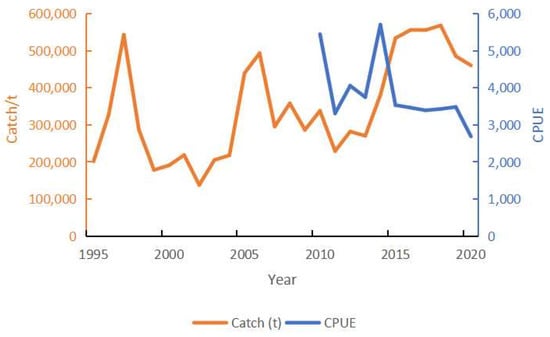
Figure 1.
Catch and CPUE of Chub mackerel in the Northwest Pacific Ocean from 1995–2020. NOTE: Catch is the total catch of all countries and fleets; CPUE is calculated as catch of purse seine fleets/number of vessels of purse seine fleets.
2.2. Stock Assessment Models and Initial Prior Parameters Settings
In this study, we used five state-space surplus production models to assess the Chub mackerel stock in the Northwest Pacific.
CMSY requires catch and resilience data, as well as quantitative stock status information [14,22]. The model fits the best r (the intrinsic rate of population increase)-K (the carrying capacity) combination from the input prior information and selects the biomass when the stock was unfished from the prior distribution of the biomass. In validating the effectiveness of the CMSY for the stock assessment of the actual fisheries, it is sometimes necessary to compare it with relevant parameters from the fully assessed stock, hence the BSM model was developed based on CMSY, which requires fishing effort data for the calculation [14,23]. The main advantage of BSM compared to other implementations of surplus production models is the focus on informative priors and the acceptance of short and incomplete (fragmented) CPUE [14,23].
We set up different scenarios for complete yield and CPUE pairings and equivalent year data to see how the results changed. For the CMSY and BSM, depletion prior ranges are very important and was classified into five categories, according to Froese et al. [14,23]. Based on previous research results [4,23], we set low depletion as the start B/K and medium depletion as the end B/K as the base case, and performed sensitivity analysis for the BSM with different prior information (Table 1). The other model settings are not described in detail in this paper (see [14]).

Table 1.
Scenarios for different parameter settings of CMSY and BSM.
The parameters estimation methods for CMSY and BSM were estimated as [25,26] MSY = rK/4, F = C/B, FMSY = 0.5r, and BMSY = 0.5K.
This study applies the CMSY+ package proposed by Froese [23], within which the CMSY and BSM models are run in an integrated manner (http://oeanrep.geomar.de/33076/, accessed on 20 October 2021).
SPiCT, a stochastic surplus production model in continuous time, incorporates dynamics in both biomass and fisheries, and observation error of both catches and biomass indices [15]. The prior information, such as K and r, can be added or not provided in the SPiCT model; therefore, in this study, two scenarios, with or without partial prior information, were set (Table 2). The other model base settings are described in detail as in [15]. The SPiCT package used in this study is from Github (https://github.com/DTUAqua/spict, accessed on 30 November 2022) [27].
Table 2.
Scenarios for different parameters settings of SPiCT.
JABBA (Just Another Bayesian Biomass Assessment) is a Bayesian state-space surplus production model with a Bayesian framework that reduces uncertainty in the model with reasonable prior information and state-space modelling that estimates both process and observation errors [16]. JABBA has already been used for stock assessment for some fisheries, such as the North Pacific Blue shark (Prionace glauca), South Atlantic Swordfish (Xiphia gladius), and Mediterranean Albacore tuna (Thunnus alalunga) [16]. JABBA-Select is a stock assessment model based on JABBA, considering fishery selectivities and life history, with the information requirement of additional gear selectivity and fish life history parameters [17]. At this stage, a few studies have been conducted on stock assessment through JABBA-Select, with only the South African silver kob (Argyrosomus inodorus) and Atlantic yellowfin tuna (Thunnus albacares) [17,28].
Here we use both the JABBA and JABBA-Select models to evaluate the effect of the presence or absence of life history parameters and selectivity on the stock status (Table 3 and Table 4). Due to the large uncertainty of selectivity estimating, four scenarios considering 0.8, 0.9, 1.1, and 1.2 times of the base selective body lengths were assumed and sensitivity analyses were conducted to explore the results of the model under different selective lengths (Table 5). The other model settings, such as the prior information on observation errors and process errors, were kept the same as for the base case settings; for details of this approach, see [14,28]. This study uses JABBA (version v1.5, https://github.com/jabbamodel/JABBA, accessed on 22 October 2021) and JABBA-Select (version v1.1, https://github.com/jabbamodel/JABBA-Select, accessed on 27 October 2021.)
Table 3.
Scenarios for different parameters settings of JABBA and JABBA-Select.
Table 4.
Summary of life history parameters and selectivity for Chub mackerel in Northwest Pacific used in the JABBA-Select.
Table 5.
Different assumptions of selectivity in the JABBA-Select for Chub mackerel in the Northwest Pacific Ocean.
2.3. Model Diagnosis and Comparison
In CMSY and BSM, if its own residual diagnostics result is green, this indicates a good fit [14,23]. The root mean squared error (RMSE) values and deviation information criteria (DIC) were used to compare the performance of model fits in JABBA and JABBA-Select models/scenarios [16,17]. The performance of the model fit in SPiCT was evaluated using one-step-ahead (OSA) residuals [29], the Ljung–Box test [30] to detect violations of the independence assumption, and the Shapiro–Wilk test [31] to detect the normality of the residuals, with tests having green shades indicating desirable results [15].
Furthermore, the problem of systematic bias in model estimates may occur as fishery data increase from year to year during the operation of a stock assessment model. The persistent over- or under-estimation of results is known as the retrospective problem [32]. This study introduced retrospective analysis to test the performances of CMSY, BSM, SPiCT, JABBA, and JABBA-Select. The Mohn’s ρ value is obtained by:
where t1 and t2 are the start and end years of the input data, respectively, t1:t indicates a fit using data from years t1–t, and X is the model parameter for a given estimate. If ρ tends to zero, this indicates that there is no retrospective problem; if ρ is greater than zero, this indicates that the estimated parameters in the long-term period are smaller than the estimates in the short-term period, and vice versa. The retrospective analysis was conducted on data from the past five years, while the Mohn’s ρ values were estimated for B/BMSY (SB/SBMSY) and F/FMSY (H/HMSY).
All analyses conducted in the present study were carried out using the R software (v4.0.3) [33].
3. Results
3.1. Model Fit
The fits for the BSM models were better, with log-residual CPUE fit values in the healthy (green) range (Figure S1). The resulting feedback for all three parameters (OSA, Ljung–Box and Shapiro–Wilk) used to validate the SPiCT models were also in the green range (Figure S2). The CPUE fits for the JABBA and JABBA-Select models were relatively similar, with the RMSE values differing by a small margin. The DIC values for the JABBA-Select selectivity scenarios did not differ by a large margin, with the DIC values for JABBA being smaller than those of the JABBA-Select scenarios (Table S1). The posterior distributions of all parameters were symmetrical and within a reasonable range, indicating that the models converged and yielded reliable results (Figures S3–S7).
3.2. Stock Dynamics and Assessment Results from Base Case Scenarios
The result of the SPiCT1 fit (Table 6) appeared to be biologically unrealistic, with an r of 4.97, and was therefore excluded from further consideration. The remaining MSY results for Chub mackerel in the Northwest Pacific varied from 0.40–0.66 million tons, with an r from 0.38–0.56. Two of the five base cases (SPiCT, JABBA) showed that the stock was not overfished in 2020; conversely the other three models indicated that it may be overfished (Table 6).
Table 6.
Posterior estimates and 95% confidence intervals of parameters for all scenarios used on Chub mackerel stock assessment in the Northwest Pacific. Numbers in red indicate the results of the spawning biomass (SB) and harvest rate (H) reported by the JABBA-Select model.
Chub mackerel biomass increased between 1995–2005 and decreased slightly after 2005, but the trend was more subdued. From 2015, the biomass trend decreased continuously until 2020; a similar trend was also witnessed for spawning biomass. The relative fishing mortality and relative harvest rates were high for Chub mackerel during 2015–2020, with much lower stock biomass and spawning biomass during this period (Figure 2 and Figure 3).
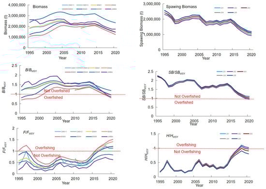
Figure 2.
Dynamic variations of stock status and biological parameters of Chub mackerel in the Northwest Pacific for CMSY, BSM, JABBA, and JABBA-Select models.
Figure 3.
Dynamic variations of stock status and biological parameters of Chub mackerel in the Northwest Pacific according to SPiCT models.
The stock status of Chub mackerel under the base case scenarios of the five models showed distinct results. The results of CMSY and BSM base cases showed that Chub mackerel stock was not in a good condition in 2020, with only 22.6% and 25.8% probabilities of being healthy, respectively. JABBA showed an 88.3% probability of Chub mackerel being in a healthy state in 2020; JABBA-Select shows a slightly worse stock status than the JABBA model, with a 46.4% probability of being in a healthy state in 2020; SPiCT did not provide the probability for each outcome, but the Kobe plot revealed that the Chub mackerel population has the highest probability of falling in the green zone. Both F/FMSY (H/HMSY) and B/BMSY (SB/SBMSY) have trended towards overfishing in recent years (Figure 4).
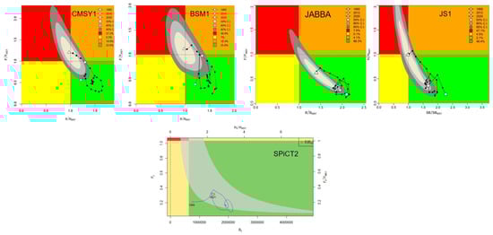
Figure 4.
Kobe phase plot showing estimated trajectories of resource state in CMSY1, BSM1, JABBA, JS1, and SPiCT2 for Chub mackerel in the Northwest Pacific. The black dotted line shows the interannual variation, and three different shades of the grey area represent the confidence intervals (C.I. 50%, 80%, 95%) of the stock status in 2020.
The retrospective analysis performed for the five base case scenarios indicated that the Mohn’s ρ values of B/BMSY and F/FMSY in SPiCT were the smallest (Table 7, Figure 5). Results of four models provided the underestimated trend of B/BMSY and SB/SBMSY, and overestimated trend of F/FMSY and H/HMSY values, while results of SPiCT were just the opposite. All five models have a retrospective pattern, with CMSY and BSMY stronger than JABBA and JABBA-Select.
Table 7.
The Mohn’s ρ values of B/BMSY, SB/SBMSY, F/FMSY, and H/HMSY of the base case scenarios of the five models for Chub mackerel in the Northwest Pacific.
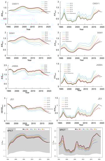
Figure 5.
Retrospective analysis of B/BMSY, SB/SBMSY, F/FMSY, and H/HMSY of the base case scenarios of the five models for Chub mackerel in the Northwest Pacific.
3.3. Sensitivity Analysis
For different data time series in CMSY1 and CMSY2, the two scenarios essentially did not show different results, whereas differences were observed between the results for B2020/BMSY and F2020/FMSY in BSM1 and BSM2. Estimates of other parameters were similar among different models. For different prior at B/K in BSM, the results of BSM1 and BSM4 were much closer together and the estimated r-values were similar in all scenarios. For the presence or absence of CPUE, the comparison of CMSY1 and BSM1 (time series 1995–2020) with CMSY2 and BSM2 (time series 2010–2020) showed almost no difference in terms of r, K, and MSY estimates, and models with the long time series (1995–2020) yielded a much closer stock status (B/BMSY, F/FMSY) (Table 6, Figure 2). For the presence or absence of the prior information, the results of SPiCT1 without prior K and r were less accurate than those of SPiCT2.
As can be seen from JABBA and JS1, the presence or absence of life history parameters and selectivity did have some effect on the model results. However, the selectivity coefficients did not have much influence on the stock assessment results, while JS1–JS2 had a slightly lower SB/SBMSY and a slightly higher H/HMSY after 2015 than those of JS3 –JS5 (Table 6, Figure 2). In addition, estimates of stock status from SPiCT and JABBA were close but more optimistic than those from CMSY, BSM, and JABBA-Select. (Table 6).
4. Discussion
In this study, we assessed the stock status of Chub mackerel in the Northwest Pacific between 1995 and 2020 (or 2010 and 2020) using five state-space surplus production models (CMSY, BSM, SPiCT JABBA, and JABBA-Select) and conducted different sensitivity runs to evaluate their performances. The results obtained in SPiCT and JABBA models indicate that the Chub mackerel stock is in a healthy state in 2020, while the CMSY, BSM, and JABBA-Select models indicate that the Chub mackerel stock may be slightly overfished. The results of the stock assessment indicate that the current MSY of Chub mackerel would be around 400,000–660,000 tonnes. The results of the sensitivity analysis indicate that the uncertainty in the JABBA-Select selectivity patterns has a small effect on the state of the stock, while the prior information of the relative biomass B/K in the BSM model has a larger effect on the final result when presenting the state of the stock.
4.1. Status of Chub Mackerel Stock
All five base cases combined show a declining trend in the stock status of Chub mackerel in the Northwest Pacific after 2015, likely due to increased fishing efforts in recent years. In 2020, the TWG CMSA started to carry out part of the stock assessment work in selecting operational models [34]. The results from the age-structured assessment program (ASAP) model indicated that MSY was between 0.14 and 0.23 million tonnes, and the corresponding Kobe plots indicated that the population was in a healthy state [19]. A Bayesian state-space biomass dynamic model (BSSPM) found Chub mackerel’s MSY to be around 1.46 million tonnes, with B2019/BMSY and F2019/FMSY of 1.53 and 0.22, respectively [35]. The MSY obtained by the Chub mackerel working group from the ASAP and BSSPM differed significantly from the results presented in the present study and the changes in biomass also differ from those obtained in this study. These differences may be characterized by the longer time series of the catch data used (1970–2019), the stock abundance index used for both studies to conduct assessments, and also because the model assumptions of ASAP are quite different from those used in the present paper. Looking at the changes in yield and nominal CPUE at this stage (Figure 1), it seems that the MSY of this study is more reasonable. However, this does not necessarily mean that a longer time series gives more accurate results; population dynamics do not necessarily stay stationary in a long time series; in such situations, stock assessment models might perform better to inform the current population status if fitted only to more recent time-series data [36].
In addition to TWG CMSA, there are few studies, especially stock assessment studies, that had been conducted on Chub mackerel in the Northwest Pacific Ocean. In recent years, only Shi et al. [9] assessed the stock status of Chub mackerel in the Northwest Pacific in 2016–2018 using a length-based Bayesian biomass evaluation (LBB), with their results indicating a healthy state (B2019/BMSY between 1.10 and 1.80). These results are in accordance with the results from 5 of the 14 scenarios tested in the present study, with the other scenarios indicating nearly full exploitation states for the Chub mackerel in the Northwest Pacific Ocean.
4.2. Uncertainty in the Stock Assessment Models
Surplus production models are known to be sensitive to different data types, especially catch time series, life history parameters, and prior values relative to the biomass and intrinsic growth rates. In this study, it seemed that the data time series duration did not show a significant influence on the results of the CMSY and BSM runs, which is in line with the conclusion observed by Kindong et al. [37] showing that differences in the catch times series did not affect the final stock status result of the South Atlantic Ocean Blue Shark (Prionace glauca). This seems to suggest that for CMSY and BSM, a particularly long time series is not required for stock assessment, but exactly how long may require further research. However, the results for BSM1 and BSM3–5 show that priors of B/K do have a significant impact on the stock status, as this may be related to the modelling style [14]. Furthermore, the change of this parameter has little effect on the results of r, K, and MSY, as observed in the present study. The similar results observed for BSM1 and BSM4 suggest that Chub mackerel’s start B2010/K set at a medium depletion level may be more accurate [14].
In the present study, SPiCT could not give accurate results without priors of K, r, as was demonstrated by the results on the species Argentine Slipper Illex argentinus [38]. Therefore, for SPiCT, the inclusion of prior information before runs is equally important for obtaining reasonable results. The different selectivity coefficients applied in the JABBA-Select model did not show very distinct significant changes, although slight differences were observed between JS1–JS2 runs and JS3–JS5 runs after 2015, which may be a result of increasing fishing efforts on the species [12]. However, studies of Atlantic Yellowfin tuna and South African silver kob have found that logistic and dome-shaped selectivity can generate a great difference in estimates of fishing mortality, absolute abundance, and stock status [17,28,39]. Although a slight difference in the harvest was observed in the present study amongst runs (JS1–5), it could be observed that the run having the smaller size at 50% retention by purse seines (JS2) indicated a possibility for this stock witnessing overfishing, thus raising the importance of properly estimating different sizes at 50% retention, as this parameter can cause variation in the final stock status results. The results of Tian et al. [28] on yellowfin tuna found that if changing the selectivity curve from a logistics curve to a dome shaped curve, it will generate differences on estimates of fishing mortality, absolute abundance, and stock status. More complex dome-shaped selectivity is worth exploring in future research when related information is available, but not limited to the logistic selectivity in this study.
Bouch et al. [40] have applied CMSY and SPiCT to 17 data-rich stocks and compared the status estimates to the accepted International Council for the Exploration of the Sea (ICES) age-based assessments. There was evidence that CMSY tended to have a negative bias relative to the ICES analytical assessments and SPiCT had a positive bias, and, importantly, both methods rarely tell the same story. This is similar to the results of this study, where CMSY showed that the stock was overfished, while SPiCT concluded that the stock was still healthy. The stock status in JABBA differed from JS1, probably because in JABBA only the shape parameter (m) can be fixed, while in JABBA-Select the best-fit m can be fitted [16,17]. Some retrospective problems were observed in the base case scenarios of the five models, with Mohn’s ρ values of B/BMSY and F/FMSY of CMSY and BSM larger than those of SPiCT, JABBA, and JABBA-Select. The difference in Mohn’s ρ values among models may be attributed to the fact that the state-space modelling of SPiCT, JABBA, and JABBA-Select can eliminate some of the uncertainty of observation errors and process errors, thus avoiding certain traceability problems [15,16,17].
4.3. Model Comparison
Since the models we use do not have uniform criteria for assessing convergence, it is difficult for us to make cross-sectional comparisons in this area (except for JABBA and JABBA-Select); however, all have their individual test criteria, which they all passed (Table S1, Figures S1 and S2). JABBA outperformed JABBA-Select in the goodness-of-fit tests (Table S1). The retrospective analysis shows that SPiCT is by far the best model in this study only, followed by JABBA and JABBA-Select, but CMSY and BSM do not perform as well here. In terms of posterior parameters feedback, CMSY and BSM performed well, but, in direct comparison, BSM would be a better choice than CMSY if CPUE data were available. The posterior parameters of SPiCT, JABBA, and JABBA-Select are all very good and almost always show a normal distribution (Figures S3–S7).
Overall, SPiCT and JABBA perform better out of these five models. SPiCT shows the most optimistic results of the five models, but as we mentioned above, SPiCT tends to be overly optimistic at times. Therefore, if we had to choose the best model, we would prefer the JABBA results. However, this does not mean that we reject the rest of the models; we prefer to give managers more scientific management advice through a slightly more flexible result obtained from multiple models.
Of our five models, CMSY requires the least amount of data [14,15,16,17]. There is no doubt that we can only use CMSY when we only have catch data, but when we have CPUE data, the surplus production model would be a better choice, as would our other four models, from our retrospective analysis and posterior results (Table 7, Figures S3–S7). The BSM is more general than SPiCT and JABBA [14,15,16] in terms of inputted a priori information and is somewhat inferior to the other two models, as revealed by retrospective analysis (Table 7). Therefore, JABBA and SPiCT can be recommended when we have more accurate prior information. Although in this paper both RMSE and DIC show that JABBA is superior to JABBA-Select, when assessing stocks from other fisheries, if we have data for JABBA-Select (Table S1), we recommend trying JABBA-Select as well.
4.4. Limitations
Compared to complex models, such as SS3 and age-structured models (ASAP), surplus production models have the characteristics of using fewer parameters and relatively simple data. However, the shape parameter has a significant effect on the estimation of K and r, and fixing the shape parameter to a certain value may affect the reliability of surplus production models [18]. Contrarily, the JABBA-Select model reduces error by using the built-in ASEM model to estimate m of spawning biomass from life history parameters; the model structure is limited by the fact that the assumed natural mortality and steepness are constant, which inevitably deviates from the true stock [17]. In order to ensure the sustainable exploitation of this stock, this study does not recommend increasing the catch. In addition, the CPUE data used in this study are not standardized, although there is also a lot of literature that uses non-standardized CPUE for calculations, as in this study [41,42], but it probably affects the accuracy of the stock assessment results to a certain extent. The standardization of CPUE data is an important basic work in the assessment and management of fishery stock [43].
The abundance and catch in the previous years (e.g., 1970s and 1980s) were extremely high [2]. After that, the fishery collapsed due to overfishing for both Japan and Russia [2]. However, the data of Chub mackerel are inconsistent among different sources, leading to difficulties for conducting stock assessments covering the early years. The data used in this research are derived from the NPFC website, limited to the year 1995 [12]. We did conduct a stock assessment to cover the early years, ignoring the inconsistent problems, but the results appeared to be confused and unrealistic, and were not added in the manuscript. If consistent data are available or there is an effective method to standardize the data, the stock assessment of Chub mackerel could cover the early years to provide more information for managers.
5. Conclusions
In this study, CMSY, BSM, SPiCT, JABBA, and JABBA-select were used to evaluate the status of Chub mackerel stock in the Northwest Pacific. The sensitivity analysis of the parameters indicated that the results differ when using different abundance data and that the prior information of the selectivity coefficients used in the JABBA-Select models slightly affect the results. Additionally, the CMSY model was more sensitive to the prior values of B/K, with SPiCT presenting unrealistic results when prior parameters were not defined. In order to improve the accuracy of the stock assessment results and reduce the uncertainty and the impact of the retrospective problem, it is necessary to focus on the quality of the catch data and the prior parameters. Though the base cases of the five stock assessment models indicate a higher likelihood that the current stock status of Chub mackerel in the Northwest Pacific might be healthy (JABBA and SPiCT) or witnessing slight overfishing (CMSY1, BSM1, and JS1), considering that Chub mackerel production has been documented to be higher in the 1970s than it is today [2], it would be preferable to maintain or slightly reduce the fishing effort to sustainably harvest this fish stock. Based on the optimistic stock status indicated from the best model, JABBA, a higher catch is allowable, but further projection is required for specific catch limit setting.
Supplementary Materials
The following supporting information can be downloaded at: https://www.mdpi.com/article/10.3390/fishes8020080/s1, Figure S1: Goodness of fitting in BSM of Chub mackerel in the Northwest Pacific; Figure S2: Goodness of fitting in SPiCT of Chub mackerel in the Northwest Pacific; Figure S3: Priors (light) and posteriors (dark) of parameters of base case in CMSY for Chub mackerel in the Northwest Pacific; Figure S4: Priors (light) and posteriors (dark) of parameters of base case in BSM for Chub mackerel in the Northwest Pacific; Figure S5: Priors (dark) and posteriors (light) of parameters in JABBA for Chub mackerel in the Northwest Pacific; Figure S6: Priors (dark) and posteriors (light) of parameters of base case in JABBA-Select for Chub mackerel in the Northwest Pacific; Figure S7: Priors and posteriors of parameters of base case in SPiCT for Chub mackerel in the Northwest Pacific; Table S1: Goodness of fitting in JABBA and JABBA-Select of Chub mackerel in the Northwest Pacific.
Author Contributions
Conceptualization, methodology, investigation, resources, writing–original draft, writing–review and editing: K.C. Data curation, investigation, conceptualization, methodology, writing–review and editing: R.K. Supervision, project administration, conceptualization, methodology, resources: Q.M. and S.T. All authors have read and agreed to the published version of the manuscript.
Funding
This study was supported by the National Natural Science Foundation of China (32202934) and the National Key R&D Programs of China (2019YFD0901404).
Institutional Review Board Statement
All applicable international, national, and/or institutional guidelines for the care and use of animals were followed.
Data Availability Statement
Data is contained within the article or supplementary materials.
Conflicts of Interest
The authors have no relevant financial or non-financial interest to disclose.
References
- Yatsu, A.; Watanabe, T.; Ishida, M.; Sugisaki, H.; Jacobson, L.D. Environmental effects on recruitment and productivity of Japanese sardine Sardinops melanostictus and Chub mackerel Scomber japonicus with recommendations for management. Fish. Oceanogr. 2005, 14, 263–278. [Google Scholar] [CrossRef]
- Yoshiue, R.; Watanabe, C.; Uemura, T.; Watanabe, C.; Taiyang, U.; Hashimoto, G. Stock Assessment of the Pacific Cohort of Chub mackerel (Scomber japonicus) in 2017; National Research Institute of Fisheries Science: Yokohama, Japan, 2017. [Google Scholar]
- Kuroda, k.; Yoda, M.; Yasuda, T.; Suzuki, K.; Takegaki, S.; Sasaki, C.; Takahashi, S. Stock Assessment of the Tsushima Current Cohort of Chub Mackerel (Scomber japonicus) in 2017; Seikai National Fisheries Research Institute: Ishigaki-jima, Japan, 2017. [Google Scholar]
- NPFC. 5th Meeting Report, NPFC-2022-TWG CMSA05-Final Report. In Proceedings of the 5th Meeting of the Technical Working Group on Chub Mackerel Stock Assessment; 2022; p. 24. Available online: https://www.npfc.int/system/files/2022-07/TWG%20CMSA05%20report.pdf (accessed on 30 November 2022).
- Nishijima, S.; Kamimura, Y.; Yukami, R.; Manabe, A. Update on Natural Mortality Estimators for Chub Mackerel in the Northwest Pacific Ocean; NPFC-2021-TWG CMSA04-WP05; North Pacific Fisheries Commission: Tokyo, Japan, 2021. [Google Scholar]
- Zhuang, P.; Wang, Y.K.; Li, S.F.; Deng, S.M.; Li, C.S.; Ni, Y. Fisheries of the Yangtze Estuary; Shanghai Scientific & Technical Publishers: Shanghai, China, 2006; pp. 361–364. [Google Scholar]
- Watanabe, C. A Review of the Reproductive Studies for Chub Mackerel in Relation to the Stock Assessment. Bull Fish Res. 2006, 4, 101–111. [Google Scholar]
- FAO. FAO Yearbook; Fishery and Aquaculture Statistics: Rome, Italy, 2022. [Google Scholar]
- Shi, Y.; Zhang, X.; He, Y.; Fan, W.; Tang, F. Stock Assessment Using Length-Based Bayesian Evaluation Method for Three Small Pelagic Species in the Northwest Pacific Ocean. Front. Mar. Sci. 2022, 9, 775180. [Google Scholar] [CrossRef]
- NPFC. 1st Meeting Report, NPFC-2017-TWG CMSA01-Final Report. In Proceedings of the 1st Meeting of the Technical Working Group on Chub Mackerel Stock Assessment; 2017; p. 21. Available online: https://www.npfc.int/system/files/2020-01/TWG%20CMSA01%20Final%20Report.pdf (accessed on 30 November 2022).
- Arnold, L.M.; Heppell, S.S. Testing the robustness of data-poor assessment methods to uncertainty in catch and biology: A retrospective approach. ICES J. Mar. Sci. 2015, 72, 243–250. [Google Scholar] [CrossRef]
- NPFC Secretariat. Summary Footprint of Chub Mackerel Fisheries. NPFC-2022-AR-Annual Summary Footprint-. Chub & Spotted Mackerels. 2022. Available online: https://www.npfc.int/summary-footprint-chub-mackerel-fisheries (accessed on 30 November 2022).
- Costello, C.; Ovando, D.; Hilborn, R.; Gaines, S.; Deschenes, O.; Lester, S. Status and Solutions for the World’s Unassessed Fisheries. Science 2012, 338, 517–520. [Google Scholar] [CrossRef]
- Froese, R.; Demirel, N.; Coro, G.; Kleisner, K.; Winker, H. Estimating fisheries reference points from catch and resilience. Fish Fish. 2017, 18, 506–526. [Google Scholar] [CrossRef]
- Pedersen, M.W.; Berg, C.W. A stochastic surplus production model in continuous time. Fish Fish. 2017, 18, 226–243. [Google Scholar] [CrossRef]
- Winker, H.; Carvalho, F.; Kapur, M. JABBA: Just another Bayesian biomass assessment. Fish. Res. 2018, 204, 275–288. [Google Scholar] [CrossRef]
- Winker, H.; Carvalho, F.; Thorson, J.; Kell, L.; Parker, D.; Kapur, M.; Sharma, R.; Booth, A.; Kerwath, S. JABBA-Select: Incorporating life history and fisheries’ selectivity into surplus production models. Fish. Res. 2020, 222, 105355. [Google Scholar] [CrossRef]
- Guan, W.; Tian, S.; Zhu, J.; Chen, X. A review of fisheries stock assessment models. J Fish Sci China. 2013, 20, 1112–1120. [Google Scholar] [CrossRef]
- Ma, Q.; Cai, K.; Tian, S.; Dai, L.; Zhou, Y. Update Stock Assessment Based on ASAP (Age-Structured Assessment Program) for Chub Mackerel in the North Pacific Ocean 2022; NPFC-2022-TWG CMSA05-WP04; North Pacific Fisheries Commission: Tokyo, Japan, 2022. [Google Scholar]
- Cai, K.; Kindong, R.; Ma, Q.; Han, X.; Qin, S. Growth Heterogeneity of Chub Mackerel (Scomber japonicus) in the Northwest Pacific Ocean. J. Mar. Sci. Eng. 2022, 10, 301. [Google Scholar] [CrossRef]
- Manabe, A.; Kamimura, Y.; Ichinokawa, M.; Oshima, K. Maturity at Age of Chub Mackerels under Different Stock Level in the Northwestern Pacific Ocean; NPFC-2021-TWG CMSA04-WP07; North Pacific Fisheries Commission: Tokyo, Japan, 2022. [Google Scholar]
- Al-Mamun, M.A.; Shamsuzzaman, M.M.; Schneider, P.; Mozumder, M.M.H.; Liu, Q. Estimation of Stock Status Using the LBB and CMSY Methods for the Indian Salmon Leptomelanosoma indicum (Shaw, 1804) in the Bay of Bengal, Bangladesh. JMSE 2022, 10, 366. [Google Scholar] [CrossRef]
- Froese, R.; Demirel, C.; Winker, H. A Simple User Guide for CMSY+ and BSM (CMSY_2019_9f. R). 2019, p. 16. Available online: http://oceanrep.geomar.de/33076/ (accessed on 30 November 2022).
- Froese, R.; Pauly, D. (Eds.) FishBase; World Wide Web Electronic Publication. 2022. Available online: www.fishbase.org (accessed on 5 April 2022).
- Schaefer, M.B. Some aspects of the dynamics of populations important to the management of the commercial marine fisheries. Int.-Am. Trop. Tuna Comm. Bull. 1954, 1, 23–56. [Google Scholar]
- Ricker, W.E. Computation and interpretation of biological statistics of fish populations. Bull. Fish. Res. Board Can. 1975, 191, 1–382. [Google Scholar]
- Pedersen, M.W.; An R-Package for Fittng Surplus Production Models in Continuous-Time to Fisheries Catch Data and Biomass Indices (Either Scientific or Commercial). v1.3.7. 2022. Available online: https://github.com/DTUAqua/spict (accessed on 30 November 2022).
- Tian, Z.; Wang, W.; Tian, S.; Ma, Q. Stock assessment for Atlantic yellowfin tuna based on extended surplus production model considering life history. Acta Oceanol. Sin. 2022, 41, 41–51. [Google Scholar] [CrossRef]
- Magnusson, A.; Hilborn, R. What makes fisheries data informative? Fish Fish. 2007, 8, 337–358. [Google Scholar] [CrossRef]
- Harvey, A.C. Foercasting, Structural Time Series Models and the Kalman Filter; Cambridge University Press: Cambridge, UK, 1989. [Google Scholar]
- Ljung, G.M.; Box, G.E.P. On a measure of lack of fit in time series models. Biometrika 1978, 65, 297–303. [Google Scholar] [CrossRef]
- Mohn, R. The retrospective problem in sequential population analysis: An investigation using cod fishery and simulated data. ICES J. Mar. Sci. 1999, 56, 473–488. [Google Scholar] [CrossRef]
- R Core Team. R: A Language and Environment for Statistical Computing; R Foundation for Statistical Computing: Vienna, Austria, 2020; Available online: https://www.R-project.org (accessed on 30 November 2022).
- NPFC. 3rd Meeting Report. NPFC-2020-TWG CMSA03-Final Report. In Proceedings of the 3rd Meeting of the Technical Working Group on Chub Mackerel Stock Assessment; 2020; p. 25. Available online: https://www.npfc.int/system/files/2021-01/TWG%20CMSA03%20report.pdf (accessed on 30 November 2022).
- Ma, Q.; Dai, L.; Cai, K.; Tian, S. North Pacific Ocean Chub Mackerel Stock Assessment Report Based on BSSPM; NPFC-2022-TWG CMSA05-WP05; North Pacific Fisheries Commission: Tokyo, Japan, 2022. [Google Scholar]
- Zhang, F.; Reid, K.B.; Nudds, T.D. The longer the better? Trade-offs in fisheries stock assessment in dynamic ecosystems. Fish Fish. 2021, 22, 789–797. [Google Scholar] [CrossRef]
- Kindong, R.; Wu, F.; Tian, S.; Ousmane, S. How Well Do ‘Catch-Only’Assessment Models Capture Catch Time Series Start Years and Default Life History Prior Values? A Preliminary Stock Assessment of the South Atlantic Ocean Blue Shark Using a Catch-Based Model. Animals 2022, 12, 1386. [Google Scholar] [CrossRef]
- Han, Q.P.; Shan, S.Q.; Guan, L.S.; Jin, X.S.; Wan, R.; Chen, Y.L. Application of SPiCT for data-limited stock assessment of short-lived Illex Argent. J. Fish. Sci. China 2018, 25, 169–177. [Google Scholar]
- Tian, Z.P.; Tian, S.Q.; Dai, L.B.; Ma, Q.Y. Stock assessment for Atlantic yellowfin tuna based on Bayesian state-space production mode. Haiyang Xuebao 2021, 43, 67–78. [Google Scholar] [CrossRef]
- Bouch, P.; Minto, C.; Reid, D.G. Comparative performance of data-poor CMSY and data-moderate SPiCT stock assessment methods when applied to data-rich, real-world stocks. ICES J. Mar. Sci. 2021, 78, 264–276. [Google Scholar] [CrossRef]
- Tian, Z.P.; Ma, Q.Y.; Zhang, Y.F.; Tian, S.Q. Uncertainties of Parameters Associated with Stock Assessment for Chub Mackerel Pneumatophoorus japonicus Based on JABBA. Fish Sci. 2022, 46, 915–926. [Google Scholar]
- Zhang, Q.Q.; Liu, Q. Assessing Biological Reference Points for Three Important Fishery Resources in Coastal Water of China. Periood. Ocean. Uni. China 2021, 51, 123–134. [Google Scholar]
- Guan, W.J.; Tian, S.Q.; Wang, X.F.; Zhu, J.W.; Chen, X.J. A review of methods and model selection for standardizing CPUE. J. Fish. Sci. China. 2014, 21, 852–862. [Google Scholar] [CrossRef]


Disclaimer/Publisher’s Note: The statements, opinions and data contained in all publications are solely those of the individual author(s) and contributor(s) and not of MDPI and/or the editor(s). MDPI and/or the editor(s) disclaim responsibility for any injury to people or property resulting from any ideas, methods, instructions or products referred to in the content. |
© 2023 by the authors. Licensee MDPI, Basel, Switzerland. This article is an open access article distributed under the terms and conditions of the Creative Commons Attribution (CC BY) license (https://creativecommons.org/licenses/by/4.0/).