The Bioeconomic Analysis of Hybrid Giant Grouper (Epinephelus fuscoguttatus × Epinephelus lanceolatus) and Green Grouper (Epinephelus malabaricus): A Case Study in Taiwan

Abstract

Grouper aquaculture is a rapidly growing and dynamic industry within the Taiwan aquaculture sector that serves as an important source of income generation. Farming fishes at a better location (FFABL) is a promising production strategy. This study evaluated the production and economic performance of grouper farming in Taiwan. This investigation employed two steps: (1) a cost–benefit analysis to determine the main component affecting profitability; and (2) multivariate statistics to clarify the relationship between biological and economic factors. The findings suggest that the best choice of species is hybrid giant grouper that generates and highlights a positive income, viable benefit–cost ratio and profit rate. The study found the feed management of hybrid giant groupers requires more consideration due to its low feed conversion ratio. The producers need to replace trash fish in commercial feed during the production cycle to ensure better feed management. Finally, this paper argues that feed is the main constraint for grouper farming, which is sensitive to any change in feed productivity, and this constraint must be solved to sustain the grouper industry in Taiwan.

1. Introduction

The aquaculture of groupers is carried out in tropical and subtropical areas throughout the world, but most production occurs in Asia. Three countries are responsible for an estimated 93% of global production, including China (65% of total production), Taiwan (17%) and Indonesia (11%) [1]. FAO reported that almost 155,000 tons of grouper were produced in 2015, with a total value of USD 630 million [2]. Grouper farming has been expanding in Taiwan, with the land area used for grouper farming increasing from 1235 ha in 2003 to 2336 ha in 2017 [3]. Consequently, grouper has emerged as one of the primary and most economically valuable species in aquaculture [4].

The application of genetics is an established approach to improving farming efficiency which has been widely applied and is increasingly used in aquaculture [5]. However, there have been studies exploring the hybridization of groupers, such as E. fuscoguttatus × E. polyphekadion [6], E. costae × E. marginatus [7], E. fuscoguttatus × E. lanceolatus [8] and E. coioides × E. lanceolatus [9]. The main appeal of hybrid groupers is increasing harvestability and environmental tolerance [10], as well as improving their growth rates [11].

Farming fishes at a better location (FFABL) is a promising production strategy which involves assessing the environmental and economic suitability of farming areas for the cultivation of major species. In terms of economic evaluation, production costs are one of the major factors affecting profitability, and the costs of fry, feed and labor are the most significant expenditures in fish farming [12,13,14,15]. Moreover, the production scale of cultivation farms can influence the input and output of the production process [16,17,18]. Different cultured species also can influence the variation in production costs, and in turn reflect the differences in profit performance. Efficient management is necessary to maximize farming profit, and analysis of the cost–return structure can, therefore, identify areas needing improvement for the cost-efficient management of farming [19].

Bio-economic analysis can provide insight into how to achieve better farming management strategies [20], which quantifies the economic implications of any change in the parameters of production and markets [21]. In this study, cost–benefit analysis was applied to evaluate farm profitability [22,23,24,25,26,27]. Multivariate analysis methods, including Mahalanobis distance and canonical discriminant function, were applied to assess variables identified as highly correlated with farm performance [15,18]. These results could provide a quantitative technique to assist producers in understanding and interpreting the many interrelated processes in grouper culture and the economic constraints faced by producers. Building upon this as a theoretical foundation, we conducted research towards the advancement of the objective of FFABL.

2. Materials and Methods

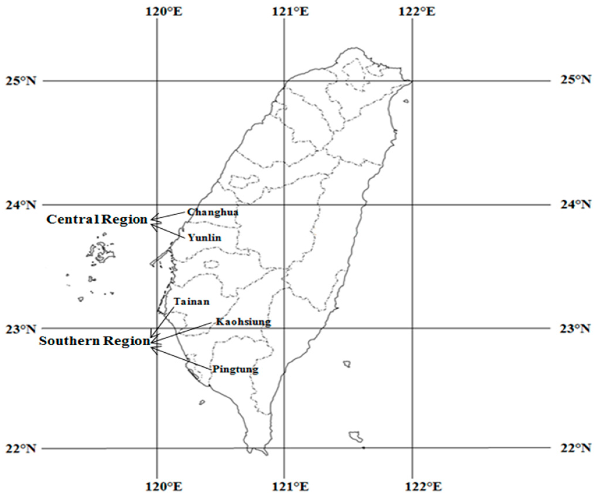
2.1. Data Input and Study Site

Two types of grouper species (green grouper and hybrid giant grouper) were evaluated in two locations (Kaohsiung and Pingtung) (Figure 1). A survey, through interviews with four-category growers, was conducted from July 2016 to March 2017. In 2017, there were a total of 1282 grouper aquaculture operators, with 382 in Kaohsiung and 467 in Pingtung. For this study, a sample of 61 operators was interviewed, comprising 29 from Kaohsiung and 32 from Pingtung.

2.2. Economic Analysis

2.2.1. Cost–Benefit Analysis

In cost–benefit analysis, the costs consist of operating expenses and depreciation costs [19,29]. Operating expenses refer to the expenses incurred in aquaculture, such as fry, water–electricity, personnel, feed, management and marketing, excluding initial investment, while depreciation costs refer to the annual amortized cost calculated by the straight-line depreciation method based on the purchase cost of hardware equipment, such as paddle wheels and water pumps. The unit is one thousand New Taiwan Dollars (NTD) per fen, with one US dollar equal to NTD 30.2. One hectare is equal to 10.31 fen (1 fen = 967 m²).

In cost–benefit analysis, cost inputs and profits are defined and calculated as follows:

(1)

Cost variables (NTD/year): cost_i/unit area (fen)

• Fry cost (FC), feed cost (FDC), labor cost (LC), water–electricity cost (WEC) and other cost (OC)

(2)

Total return (TR) (NTD/year): stocking density (piece/fen) × survival rate (%) × harvest size (kg/piece) × purchasing price (NTD/kg)

(3)

Total cost (TC)(NTD/year): fry cost + feed cost + personnel cost + water–electricity cost + other costs (NTD/year)

(4)

Net return (NR) (NTD/year): total earning (NTD/year)-total cost (NTD/year)

(5)

Benefit–cost ratio (BCR): BCR_n = NR_n/TC_n

n: the n^th year

BCR_n: Benefit–cost ratio in the n^th year

NR_n: Net return in the n^th year

TC_n: Total cost in the n^th year

(6)

Profit rate (PR): PR_n = NR_n/TR_n

n: the n^th year

PR_n: Profit rate in the n^th year

NR_n: Net return earning in the n^th year

TR_n: Total return in the n^th year

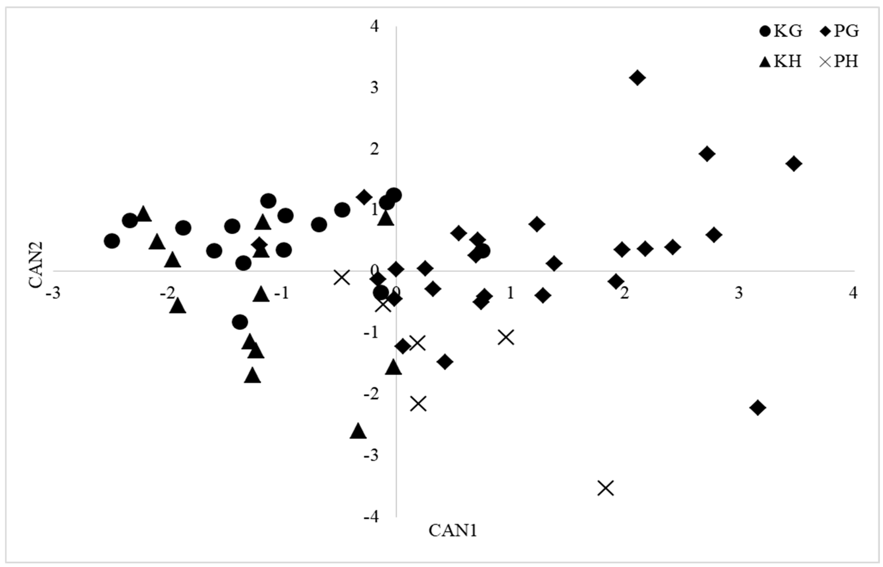
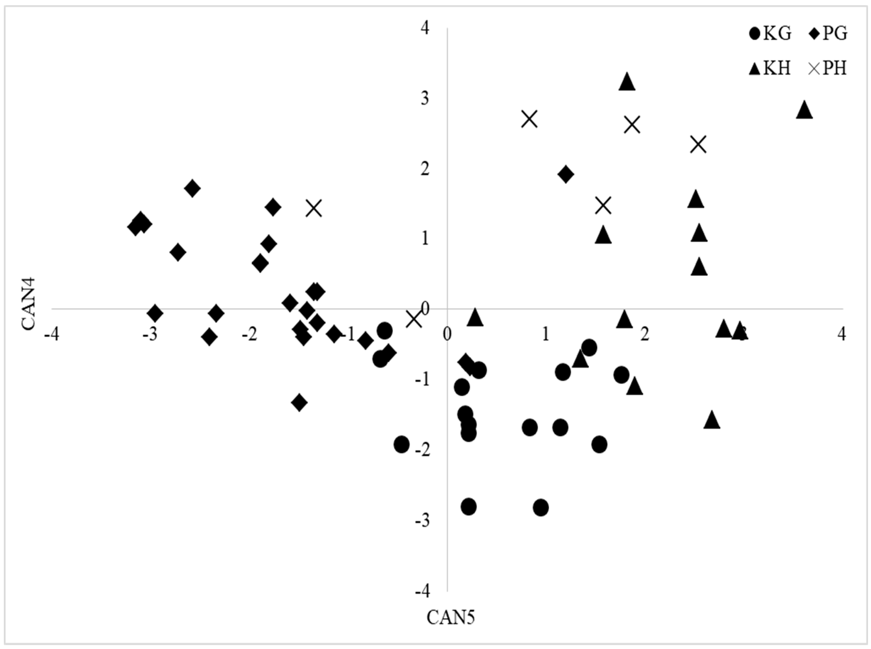
2.2.2. Multivariate Analysis

The effects of geographical location and species on profitability performance were examined by multivariate analyses. We conducted a test of the null hypothesis that the main effect means (expressed in mean vectors) caused by the factor of geographical location would not be statistically different. The test was as follows: H₀: u_L = u_S, where ‘u_L’ refers to the location factor and ‘u_S’ refers to the species factor. This analysis was applied to three key variables: biological variables, input intensities and profitability variables, including a two-way analysis of variance (ANOVA) that considered the studied factors of location, species and the interaction between these groups. Subsequently, a two-way ANOVA was employed to further analyze variables that exhibited significant differences, exploring the specific factors influencing these variables.

Mahalanobis Distances and Canonical Discriminant Function

The Mahalanobis distances among the four categories were first calculated using biological variables, input intensities and profitability variables, respectively, to validate the differences in farming performance [30]. These were calculated as follows.

$$D_{ij}^2=({\overline{x}}_i-{\overline{x}}_j)\prime C^{-1}\left({\overline{x}}_i-{\overline{x}}_j\right),$$

where $D_{ij}^2$ is the Mahalanobis distance between category i and category j, ${\overline{x}}_i$ is a mean vector of the ith category with dimensions of 4 × 1 and $C^{-1}$ is a unique inverse of variance–covariance matrix C with dimensions of 4 × 4.

The canonical discriminant function was used to find linear combinations of the quantitative variables providing maximal separation among the locations and species. The first few functions were expected to be sufficient to account for almost all of the important group differences, and the canonical discriminant functions were sufficient to account for almost all of the important differences in farms [31]. This was calculated as follows.

$${CAN}_i={\alpha }_1{X}_1+{\alpha }_2{X}_2+{\alpha }_3{X}_3+\cdots +{\alpha }_n{X}_n,$$

where $X_n$ indicates fry cost, feed cost, labor cost, water–electricity cost and other cost as input intensity variables, and mean total revenue, net revenue, benefit cost ratio and profit rate as profitability variables.

Cobb-Douglas Production Function

The Cobb–Douglas production function was used to study the quantitative relationship between the inputs and output of the production system. Carefully evaluating this quantitative relationship helped to measure the responsiveness of the output to a unit increase in the inputs. The production function would exhibit increasing returns to scale if ε > 1; i.e., a simultaneous increase in all inputs by a certain percentage would result in a greater percentage increase in the output. If ε = 1, the production function would exhibit constant returns to scale; i.e., a simultaneous increase in all inputs by a certain percentage would result in an increase in production by the same percentage. If ε < 1, the production function would exhibit decreasing returns to scale; i.e., the proportional increase in the output would be less than the proportional increase in all inputs [23]. Computer software developed by the SAS Institute was adopted for this analysis.

3. Results

Table 1. Original variables of geographical location and species for green grouper and hybrid giant grouper farms in Taiwan.

	Geographical Location		Species
	Kaohsiung	Pingtung	Green Grouper	Hybrid Giant Grouper
Number of farms (n)	29	32	42	19
Farming area (fen)	13.6 ± 20.9	10.4 ± 11.8	11.7 ± 17.7	12.4 ± 14.6
Biological variables
Stocking density (pcs/fen)	5287.3 ± 1460.4	11,584.4 ± 2140.0	9286.5 ± 3548.2	7052.6 ± 3523.3
Survival rate (%)	68.9 ± 15.9	64.4 ± 11.3	64.3 ± 12.8	71.4 ± 14.9
Farming cycle (month)	15.7 ± 3.3	15.2 ± 2.6	16.8 ± 2.3	12.6 ± 2.1
Input intensities (NTD 1000/fen)
Fry cost (FC)	116.3 ± 58.8	199.4 ± 63.6	155.2 ± 66.7	170.2 ± 88.6
Feed cost (FDC)	321.5 ± 107.1	561.5 ± 142.7	475.8 ± 173.7	384.6 ± 163.8
Water–electricity cost (WEC)	38.3 ± 18.6	68.5 ± 39.9	63.0 ± 38.2	34.5 ± 11.2
Labor cost (LC)	43.3 ± 27.4	72.9 ± 40.8	64.8 ± 40.5	45.7 ± 27.8
Other cost (OC)	17.1 ± 10.9	23.2 ± 13.2	21.1 ± 13.7	18.5 ± 9.2
Total cost	536.7 ± 160.6	925.4 ± 200.9	780.0 ± 269.8	653.5 ± 244.7
Profitability variables
Total revenue (TR) (NTD 1000/fen)	799.0 ± 359.4	1152.1 ± 423.4	884.5 ± 354.1	1204.9 ± 504.9
Net revenue (NR) (NTD 1000/fen)	262.4 ± 258.1	226.7 ± 359.3	104.4 ± 184.0	551.4 ± 323.7
Benefit–cost ratio (BCR)	0.47 ± 0.40	0.25 ± 0.42	0.13 ± 0.22	0.84 ± 0.35
Profitability rate (PR)	0.27 ± 0.18	0.13 ± 0.22	0.09 ± 0.16	0.44 ± 0.11

Values are expressed as mean ± SD.

summarizes the basic statistical data related to biological and economic variables, distinguished by location (Kaohsiung and Pingtung) and species (hybrid giant grouper and green grouper) of grouper aquaculture in Taiwan. The means and standard deviations of the original biological variables, input intensities and profitability variables in the four farming categories are listed in

Table 2. Original variables of four-category grouper farms in Taiwan.

	Kaoshiung		Pingtung
	Green Grouper	Hybrid Giant Grouper	Green Grouper	Hybrid Giant Grouper
Number of farms (n)	16	13	26	6
Farming area (fen)	17.5 ± 27.1	8.7 ± 6.8	8.0 ± 5.9	20.2 ± 23.3
Biological variables
Stocking density (pcs/fen)	5552.1 ± 1673.0	4961.5 ± 1126.6	11,584.6 ± 2133.1	11,583.3 ± 2375.2
Survival rate (%)	64.1 ± 15.2	74.8 ± 15.4	64.4 ± 11.4	64.2 ± 11.6
Farming cycle (month)	17.8 ± 2.7	13.2 ± 2.1	16.1 ± 1.9	11.3 ± 1.6
Input intensities (NTD 1000/fen)
Fry cost (FC)	99.1 ± 42.4	137.5 ± 70.3	189.7 ± 54.5	241.2 ± 87.1
Feed cost (FDC)	319.9 ± 96.8	323.5 ± 122.7	571.7 ± 136.8	517.0 ± 172.5
Water–electricity cost (WEC)	45.0 ± 22.0	30.1 ± 8.1	74.1 ± 42.0	43.9 ± 11.7
Labor cost (LC)	48.0 ± 30.7	37.6 ± 22.6	75.2 ± 42.8	63.2 ± 31.9
Other cost (OC)	18.1 ± 12.9	16.0 ± 8.2	23.0 ± 14.1	23.9 ± 9.5
Total cost	530.1 ± 157.6	544.7 ± 170.4	933.8 ± 199.8	889.1 ± 220.2
Profitability variables
Total revenue (TR) (NTD 1000/fen)	562.1 ± 204.4	936.9 ± 416.8	1033.8 ± 339.5	1660.7 ± 395.2
Net revenue (NR) (NTD 1000/fen)	110.0 ± 94.7	449.9 ± 274.1	101.0 ± 223.8	771.4 ± 334.5
Benefit–cost ratio (BCR)	1.23 ± 0.18	1.88 ± 0.31	1.10 ± 0.24	1.91 ± 0.42
Profitability rate (PR)	0.15 ± 0.12	0.43 ± 0.10	0.06 ± 0.17	0.45 ± 0.14

Values are expressed as mean ± SD.

. Notably, our focus in Table 1 and Table 2 centers on survival rates and feed costs derived from data gathered during on-site interviews with aquaculture farmers, capturing essential information regarding various variables.

A two-way multivariate analysis of variance (MANOVA) indicated that the studied factors of location and species had significant effects on the biological variables, input intensities and profitability variables, and their interactions had significant effects on profitability variables (

Table 3. Two-way MANOVA (biological variables, input intensities and profitability variables) of geographical location and species for green grouper and hybrid giant grouper aquafarms in Taiwan.

	Biological Variables		Input Intensities		Profitability Variables
Number of factors	F value	Pr > F	F value	Pr > F	F value	Pr > F
Location (L)	53.60	<0.0001	9.39	<0.0001	25.70	<0.0001
Species (S)	18.88	<0.0001	4.21	0.0027	29.83	<0.0001
L × S	0.74	0.5337	0.44	0.8216	8.83	<0.0001

). The results demonstrated that the location had a statistically significant effect on the stocking density (p < 0.0001) and farming cycle (p = 0.0068), and the species also had a significant effect on the farming cycle (p = 0.0001) (

Table 4. Two-way ANOVA analysis of geographical location and species for green grouper and hybrid giant grouper aquafarms in Taiwan (biological variables).

Factor (s)	Stocking Density		Survival Rate		Farming Cycle
	F-Value	Pr > F	F-Value	Pr > F	F-Value	Pr > F
Location (L)	133.00	<0.0001	1.70	0.1981	7.88	0.0068
Species (S)	0.29	0.5917	1.76	0.1893	56.57	<0.0001
L × S	0.29	0.5933	1.94	0.1688	0.03	0.8656

). The results showed that the location had statistically significant effect on the fry cost, feed cost and total cost (p < 0.0001) (

Table 5. Two-way ANOVA of geographical location and species for green grouper and hybrid giant grouper aquafarms in Taiwan (input intensities).

Factor (s)	Input Intensities
	Fry		Feed		Water–Electricity		Labor		Other
	F-Value	Pr > F	F-Value	Pr > F	F-Value	Pr > F	F-Value	Pr > F	F-Value	Pr > F
Location (L)	31.46	<0.0001	34.97	<0.0001	5.74	0.0198	6.46	0.0138	3.13	0.0823
Species (S)	6.71	0.0121	0.46	0.4997	6.38	0.0144	1.16	0.2865	0.03	0.8637
L × S	0.14	0.7062	0.60	0.4412	0.73	0.3964	0.01	0.9377	0.16	0.6939

). Furthermore, the species had a statistically significant effect on the profitability variables (p < 0.0001), and the location had significant effects on the total and net revenue (

Table 6. Two-way ANOVA analysis of geographical location and species for green grouper and hybrid giant grouper farming in Taiwan (profitability variables).

Factor (s)	Profitability Variables
	Total Revenue		Net Revenue		Benefit–Cost Ratio		Profitability Ratio
	F Value	Pr > F	F Value	Pr > F	F Value	Pr > F	F Value	Pr > F
Location (L)	29.23	<0.0001	5.67	0.0206	0.00	0.9450	0.60	0.4416
Species (S)	24.96	<0.0001	59.29	<0.0001	82.27	<0.0001	67.04	<0.0001
L × S	1.91	0.1722	6.35	0.0146	1.54	0.2199	1.78	0.1873

).

The Mahalanobis distances which computed the input intensity variables highlighted significant differences in the management performances among the four categories (

Table 7. A matrix of Mahalanobis distances ¹ of input intensity variables between four categories of green grouper and hybrid giant grouper aquafarms in Taiwan.

	Pingtung Green Grouper (PG)	Pingtung Hybrid Giant Grouper (PH)	Kaohsiung Green Grouper (KG)	Kaohsiung Hybrid Giant Grouper (KH)
Pingtung green grouper (PG)	0 2 (1.0000) 3
Pingtung hybrid giant grouper (PH)	3.1829 (0.0102)	0 (1.0000)
Kaohsiung green grouper (KG)	4.7402 (<0.0001)	6.0525 (0.0003)	0 (1.0000)
Kaohsiung hybrid giant grouper (KH)	5.9635 (<0.0001)	3.7759 (0.0102)	1.0510 (0.1452)	0 (1.0000)

¹ Mahalanobis distance was expressed considering five input intensity variables, including fry cost, feed cost, labor cost, water–electricity cost and other costs as a whole. ² The values in the table represent Mahalanobis distances, providing a measure of the distance between each data point and the group mean. ³ The values represent the p-values of Mahalanobis distances, indicating the statistical significance of the distance between each data point and the group mean.

). Nevertheless, the distances computed using profitability variables all showed significant differences across locations and species (

Table 8. A matrix of Mahalanobis distances ¹ of profitability variables between four categories of green grouper and hybrid giant grouper aquafarms in Taiwan.

	Pingtung Green Grouper (PG)	Pingtung Hybrid Giant Grouper (PH)	Kaohsiung Green Grouper (KG)	Kaohsiung Hybrid Giant Grouper (KH)
Pingtung green grouper (PG)	0 2 (1.0000) 3
Pingtung hybrid giant grouper (PH)	10.8806 (<0.0001)	0 (1.0000)
Kaohsiung green grouper (KG)	7.7746 (<0.0001)	11.2238 (<0.0001)	0 (1.0000)
Kaohsiung hybrid giant grouper (KH)	14.6948 (<0.0001)	7.5953 (<0.0001)	7.5752 (<0.0001)	0 (1.0000)

¹ Mahalanobis distance was expressed considering profitability variables, including total revenue, net revenue, benefit–cost ratio and profit rate as a whole. ² The values in the table represent Mahalanobis distances, providing a measure of the distance between each data point and the group mean. ³ The values represent the p-values of Mahalanobis distances, indicating the statistical significance of the distance between each data point and the group mean.

).

Canonical discriminant function analysis was performed by considering the input intensities and profitability variables across locations and species (

Table 9. Canonical discriminant function analysis of four categories based on input intensities.

Canonical Coefficients	CAN1	CAN2	CAN3
Fry cost (FC)	0.1028	−1.0622	0.3911
Feed cost (FDC)	0.6771	0.3165	−0.8131
Water−electricity cost (WEC)	0.3771	0.5013	0.2720
Labor cost (LC)	0.3881	0.2217	0.8470
Other costs (OC)	0.1028	−1.0622	0.3911
Eigenvalue	1.2349	0.3651	0.0043
Approximated F value	6.29	3.13	0.12
Pr > F	<0.0001	0.0071	0.8860
Means of canonical variables
Pingtung green grouper (PG)	1.1346	0.2006	−0.0213
Pingtung hybrid giant grouper (PH)	0.4295	−1.4328	0.1099
Kaohsiung green grouper (KG)	−1.0108	0.5610	0.0637
Kaohsiung hybrid giant grouper (KH)	−1.2234	−0.4304	−0.0865

). The canonical variables were as follows:

CAN1 = 0.1028FC + 0.6771FDC + 0.3771WEC + 0.3881LC + 0.1028OC

CAN2 = −1.0622FC + 0.3165FDC + 0.5013WEC + 0.2217LC − 1.0622OC

A plot of CAN1 against CAN2 would assist in recognizing the differences among grouper farms across locations and species by input intensities through a visual aid (Figure 2). Canonical profitability variables across locations and species (

Table 10. Canonical discriminant function analysis of four categories based on profitability variables.

Canonical Coefficients	CAN4	CAN5	CAN6
Total revenue (TR)	−1.3112	1.4857	1.0115
Net revenue (NR)	0.7824	−1.6170	−3.4639
Benefit−cost ratio (BC)	0.0532	2.0186	2.4178
Profitability rate (PR)	0.8662	−0.9136	−0.1496
Eigenvalue	2.4303	0.9817	0.3683
Approximated F value	15.79	11.86	10.31
Pr > F	<0.0001	<0.0001	0.0002
Means of canonical variables
Pingtung green grouper (PG)	−1.6127	0.2490	0.2141
Pingtung hybrid giant grouper (PH)	0.8609	1.7364	−1.3824
Kaohsiung green grouper (KG)	0.5220	−1.4427	−0.3817
Kaohsiung hybrid giant grouper (KH)	−1.2234	−0.4304	−0.0865

) were also determined as follows:

CAN4 = −1.3112TR + 0.7824NR + 0.0532BC + 0.8662PR

CAN5 = 1.4857TR − 1.6170NR + 2.0186BC − 0.9136PR

Figure 3 shows the distribution of grouper farms according to locations and species through profitability variables.

Using the Cobb–Douglas function, various methods (i.e., forward selection, backward elimination, stepwise, adjusted R² selection and Mallows’ C_p selection) were analyzed at the same time to estimate the relationship between total production (TP) and the five cost inputs, including fry (FC), feed (FDC), water–electricity (WEC), labor (LC) and other costs (OC). This method showed that only the feed cost had significant effects (p < 0.0001) on the total production of green grouper and hybrid grouper, with elasticities of 1.0156 and 0.9045, respectively (

Table 11. The Cobb–Douglas production function, ¹ estimated by relating ² unit return to input intensities for green grouper aquafarms in Taiwan.

Parameter	Constant/Input Intensity
	Constant	Feed Cost (FDC)	Labor Cost (LC)	Other Costs (OC)
	Log β0	β1	β2	β3
Estimated parameter	−4.7708	1.0156	0.1019	−0.0559
Standard error	0.9880	0.0788	0.0616	0.0461
t value	23.31	165.96	2.74	1.47
Pr > |t|	<0.0001	<0.0001	0.1061	0.2331

¹ This function was determined as TP = β₀(FDC) ^β1 (LC) ^β2 (OC) ^β3, where TP is a unit return (Taiwanese kilogram/fen). ² R² = 0.8627 and C(p) = 2.2286.

and

Table 12. The Cobb–Douglas production function ¹ estimated by relating ² unit return to input intensities for hybrid grouper aquafarms in Taiwan.

Parameter	Constant/Input Intensity
	Constant	Feed Cost (FDC)	Labor Cost (LC)	Other Cost (OC)
	Log β0	β1	β2	β3
Estimated parameter	−6.7409	0.9045	0.2773	0.1125
Standard error	2.4894	0.1814	0.2353	0.1116
t value	7.33	24.86	1.39	1.02
Pr > |t|	0.0162	0.0002	0.2568	0.3296

¹ This function was determined as TP = β₀(FDC) ^β1 (LC) ^β2 (OC) ^β3, where TP is a unit return (Taiwanese kilogram/fen). ² R² = 0.8627 and C(p) = 2.2286.

). The equations used for green and hybrid giant grouper were TP = 8.4735 × 10⁻³ × FDC^1.0156 and TP = 1.1815 × 10⁻³ × FDC^0.9045, respectively.

4. Discussion

This study demonstrates that producers in Pingtung have stock of either green or hybrid giant grouper of over 10,000 pcs/fen compared to producers in Kaohsiung, which are stocked at 5000 pcs/fen. The survival rate, apart from that of hybrid giant grouper in Kaohsiung, is below 65% (Table 2). Similarly to other studies, it was found that groupers are carnivorous fish; most of the mortality occurs within the first month after stocking, with a survival rate below 75% [12]. In this study, we found that the farmers stocked 5–6 cm of fry of both species. Selection of the appropriate fry size in grouper culture is extremely crucial, and increasing the fry size improves the survival rate of both species. The preferred fry size for stocking is above 7 cm, given that grouper fry are highly cannibalistic [32]. From an economic standpoint, a better survival rate would increase farming production and therefore increase revenue. However, a small fry size increases their susceptibility to environmental fluctuations, and this vulnerability intensifies during the transition of grouper fry from the nursery to net cages for their grow-out phase, particularly within the first week. The increased risk of diseases at this stage is attributed to various stressors, including handling, sorting, transportation, packing, stocking density, and the health status of fry during the nursery or captive stages [33]. Furthermore, the effect of the farming cycle from an economic perspective is significant in the farming business. The farming cycle for hybrid giant grouper farming in both locations is between 11 and 13 months, but this takes 16 to 17 months for green grouper. Longer production periods in fish culture normally cause increasing costs, while shorter cycles lead to economic profits [20]. Finally, the findings of the present study demonstrate that a better fry quality will improve the survival rate, and that the hybrid giant grouper is the best choice of species due to its shorter farming cycle.

In this study, the cost variables, including fry, feed, labor, water–electricity and others, were measured. Feed cost was found to be the largest expense for commercial grouper farming, ranging from 57% to 61% over locations and species (Table 1 and Table 2). This finding resonates with established assertions that highlight feed costs constituting 30% to 60% of the total production costs in tilapia farming [34]. Moreover, a parallel scenario was observed in Taiwan, where feed costs represent the dominant proportion in the total production costs of Eleutheronema tetradactylum cultivation [35]. In a similar vein, bioeconomic studies on hybrid grouper farming in Vietnam have revealed that feed costs account for 68% to 74% of the total costs [36]. Commercial feed is the primary feed source for green grouper, and producers apply reasonable feed management in the range of 1.5 to 2.0 for the current feed conversion ratio. It is inferred that green grouper producers have strict control over feed management. On the other hand, the feed conversion ratio (FCR) for hybrid giant grouper of 3.0 to 6.0 as trash fish represents the most common source of feed. FCR was calculated as the ratio of the feed weight provided over a certain period to the corresponding increase in body weight. A lower FCR indicated more efficient feed utilization. According to the research reports, an FCR of 3.6 was obtained for 1.2 kg of harvested fish, and the FCR range for grouper cage cultures was between 6 and 17 [1,37,38]. The FCR when using low-value finfish ranged from 9 to 12 for grouper farming in Vietnam [36].

Fry constitutes the second major expense for the grouper farming business. The unit price of green grouper and hybrid giant grouper range from NTD 12 to 26 and from NTD 13 to 35 per fry, respectively. The cost difference across species results from different degrees of success in hatching. The survival of groupers in hatchery systems is generally very low when compared to other finfish [39,40]. Moreover, high mortality during the early larval stages has been observed in most grouper species reared in hatcheries [7,41,42,43,44]. The limited availability of hybrid fingerlings is a major constraint on the grouper aquaculture industry, as larval mortality rates are high and seed cost is high. The high seed costs are a result of the limited number of grouper hybrid eggs [36]. Therefore, giant hybrid producers must consider using commercial feed in the future to improve feed management, as well as stocking fry of the proper size to compensate for the expensive fry price.

The profit indices representing business performance analyzed in this study included total revenue, net revenue and BCR. The evidence obtained from grouper cultures proved that the hybrid giant grouper retained a high BCR (1.88–1.91) and PR (0.43–0.45). These indices are almost similar to the BCR index of a humpback grouper culture in Indonesia [12]. This performance of the profitability index was mainly related to the sales price. Since the hybrid giant grouper’s sales price was higher than green grouper, therefore, the hybrid giant grouper had higher BCR and PR values. Finally, this study reveals that hybrid giant grouper is the first choice of species due to its strong market demand, sales prices, fast growth rate and shorter production cycle compared to green grouper.

Mahalanobis distance and the canonical discriminant function were applied to measure distances, which were computed using input intensities and profitability variables. These analyses revealed that the fry and feed costs are the main expenses in hybrid giant grouper cultures, as shown in Figure 2. The figure demonstrated that hybrid giant grouper farms are distributed at higher CAN1 (positive sign) and higher CAN2 (negative sign) scores, indicating that these farms spend more on fry and feed costs. Figure 3 shows that hybrid giant grouper farms had higher CAN4 and CAN5 scores. This indicates that hybrid giant grouper cultures retain better BCR and PR indices. These results support the evidence mentioned previously that hybrid giant grouper exhibits a better economic performance.

Cobb–Douglas function analysis revealed that the key variable influencing production was strongly determined by the feed cost. The analysis revealed that the green grouper unit return decreases by 1% if the feed component increases by 1.0156%. It could be said that the profit generated from production decreases if producers cannot properly manage the feeding protocol during the production cycle. A similar trend was highlighted in hybrid giant grouper farming: the unit decreases when feed expenses are increased. These results reveal that feed is the main constraint on Taiwan grouper farming and is very sensitive to any change in productivity. An increase in FCR would positively increase the cost of producing a kilogram of grouper [45]. Inefficient use of trash fish causes grouper producers to have less control over feeding management [12]. As a result, the feed management of both grouper species allow aquaculture to improve in the future in order to sustain the grouper industry in Taiwan.

5. Conclusions

The results of this study indicate that location, species and management factors have significant impacts on the biological, economic and profitability variables in grouper aquaculture. To enhance the economic viability and sustainability of grouper farming, it is recommended to improve feed management, select appropriate fry sizes for stocking and emphasize cost control and production cycles.

Furthermore, the findings highlight that feed is a critical limiting factor for both green and hybrid giant grouper species, and its productivity is highly sensitive to any changes. Therefore, implementing feeding protocols and transitioning from trash fish to commercial feed are crucial steps toward better feed management.

Moreover, this study reveals that hybrid giant grouper farming demonstrates a more positive income, a viable benefit–cost ratio and superior profit rates. Thus, when considering the choice of species for aquaculture, the hybrid giant grouper stands out due to its strong market demand, higher selling prices, faster growth rate and shorter production cycle.

In summary, this study emphasizes the influence of location, species and management factors on various aspects of grouper aquaculture, including biological, economic and profitability variables. Improving feed management, selecting appropriate fry sizes and focusing on cost control and production cycles will contribute to enhancing the economic benefits and sustainability of grouper farming in the future.

As the present study focuses on the analysis of the grouper aquaculture industry in Taiwan based on data collected from 2016 to 2017, the limitations may include the influence of temporal and spatial factors. In the future, we plan to combine recent survey data with information on other significant aquaculture species, integrating data from previous years to explore strategies for FFABL.

References

1. Rimmer, M.A.; Glamuzina, B. A review of grouper (Family Serranidae: Subfamily Epinephelinae) aquaculture from a sustainability science perspective. Rev. Aquac. 2019, 11, 58–87. [Google Scholar] [CrossRef]
2. FAO. FishStatJ, a Tool for Fisheries Statistics Analysis; FAO Fisheries and Aquaculture Department, FIPS-Statistics and Information: Rome, Italy, 2017. [Google Scholar]
3. Fisheries Annual Report 2018. Annual Report of Fishery Statistics; Fisheries Department of the Council of Agriculture, Executive Yuan: Taipei, Taiwan, 2018. [Google Scholar]
4. Chen, J.C.; Chen, T.L.; Wang, H.L.; Chang, P.C. Underwater abnormal classification system based on deep learning: A case study on aquaculture fish farm in Taiwan. Aquac. Eng. 2022, 99, 102290. [Google Scholar] [CrossRef]
5. Gjedrem, T.; Robinson, N.; Rye, M. The importance of selective breeding in aquaculture to meet future demands for animal protein: A review. Aquaculture 2012, 350–353, 117–129. [Google Scholar] [CrossRef]
6. James, C.M.; Al-Thobaiti, S.A.; Rasem, B.M.; Carlos, M.H. Potential of grouper hybrid (Epinephelus fuscoguttatus × E. polyphekadion) for aquaculture. ICLARM Q. 1999, 22, 19–23. [Google Scholar]
7. Glamuzina, B.; Glavić, N.; Skaramuca, B.; Kožul, V.; Tutman, P. Early development of the hybrid Epinephelus costae ♀ × E. marginatus ♂. Aquaculture 2001, 198, 55–61. [Google Scholar] [CrossRef]
8. Ch’ng, C.L.; Senoo, S. Egg and larval development of a new hybrid grouper, tiger grouper Epinephelus fuscoguttatus × giant grouper E. lanceolatus. Aquac. Sci. 2008, 56, 505–512. [Google Scholar] [CrossRef]
9. Chu, K.I.C.; Shaleh, S.R.M.; Akazawa, N.; Oota, Y.; Senoo, S. Egg and larval development of a new hybrid orange-spotted grouper Epinephelus coioides × giant grouper E. lanceolatus. Aquac. Sci. 2010, 58, 1–10. [Google Scholar] [CrossRef]
10. Bartley, D.M.; Rana, K.; Immink, A.J. The use of inter-specific hybrids in aquaculture and fisheries. Rev. Fish Biol. Fish. 2001, 10, 325–337. [Google Scholar] [CrossRef]
11. Huang, W.; Liu, Q.; Xie, J.; Wang, W.; Xiao, J.; Li, S.; Zhang, H.; Zhang, Y.; Liu, S.; Lin, H. Characterization of triploid hybrid groupers from interspecies hybridization (Epinephelus coioides ♀ × Epinephelus lanceolatus ♂). Aquac. Res. 2014, 47, 2195–2204. [Google Scholar] [CrossRef]
12. Afero, F.; Miao, S.; Perez, A.A. Economic analysis of tiger grouper Epinephelus fuscoguttatus and humpback grouper Cromileptes altivelis commercial cage culture in Indonesia. Aquac. Int. 2010, 18, 725–739. [Google Scholar] [CrossRef]
13. Huang, C.T.; Miao, S.; Nan, F.H.; Jung, S.M. Study on regional production and economy of cobia Rachycentron canadum commercial cage culture. Aquacult Int. 2011, 19, 649–664. [Google Scholar] [CrossRef]
14. Mohammad, T.; Moulick, S.; Mukherjee, C.K. Economic feasibility of goldfish (Carassius auratus Linn.) recirculating aquaculture system. Aquac. Res. 2018, 49, 2945–2953. [Google Scholar] [CrossRef]
15. Nguyen, P.V.; Huang, C.T.; Hieu, T.K.; Hsiao, Y.J. Economic evaluation for improving productivity of brine shrimp Artemia franciscana culture in the Mekong Delta, Vietnam. Aquaculture 2020, 526, 735425. [Google Scholar] [CrossRef]
16. Miao, S.; Tang, H.C. Bioeconomic analysis of improving management productivity regarding grouper Epinepelus malabaricus farming in Taiwan. Aquaculture 2002, 211, 151–169. [Google Scholar] [CrossRef]
17. Miao, S.; Jen, C.C.; Huang, C.T.; Hu, S.H. Ecological and economic analysis for cobia Rachycentron canadum commercial cage culture in Taiwan. Aquac. Int. 2009, 17, 125–141. [Google Scholar] [CrossRef]
18. Huang, C.T.; Nguyen, P.V.; Chen, Y.T.; Liang, T.T.; Nan, F.H.; Liu, P.C. Improving productivity management of commercial abalone Haliotis diversicolor supertexta and Haliotis discus hannai aquaculture in Taiwan: A bioeconomic analysis. Aquaculture 2019, 512, 734323. [Google Scholar] [CrossRef]
19. Huang, C.-T.; Afero, F.; Hung, C.-W.; Chen, B.-Y.; Nan, F.-H.; Chiang, W.-S.; Tang, H.-J.; Kang, C.-K. Economic feasibility assessment of cage aquaculture in offshore wind power generation areas in Changhua County, Taiwan. Aquaculture 2022, 548, 737611. [Google Scholar] [CrossRef]
20. Shinji, J.; Nohara, S.; Yagi, N.; Wilder, M. Bio-economic analysis of super-intensive closed shrimp farming and improvement of management plans: A case study in Japan. Fish. Sci. 2019, 85, 1055–1065. [Google Scholar] [CrossRef]
21. Llorente, I.; Luna, L. Bioeconomic modelling in aquaculture: An overview of the literature. Aquac. Int. 2016, 24, 931–948. [Google Scholar] [CrossRef]
22. Campbell, H.F.; Brown, R.P.C. A multiple account framework for cost–benefit analysis. Eval. Program Plan. 2005, 28, 23–32. [Google Scholar] [CrossRef]
23. Engle, C.R. Aquaculture Economics and Financing Management and Analysis; Wiley-Blackwell: Ames, IA, USA, 2010; pp. 163–165. [Google Scholar]
24. Farel, R.; Yannou, B.; Ghaffari, A.; Leroy, Y. A cost and benefit analysis of future end-of-life vehicle glazing recycling in France: A systematic approach. Resour. Conserv. Recycl. 2013, 74, 54–65. [Google Scholar] [CrossRef]
25. Dalton, G.; Bardócz, T.; Blanch, M.; Campbell, D.; Johnson, K.; Lawrence, G.; Lilas, T.; Friis-Madsen, E.; Neumann, F.; Nikitas, N.; et al. Feasibility of investment in Blue Growth multiple-use of space and multi-use platform projects; results of a novel assessment approach and case studies. Renew. Sustain. Energy Rev. 2019, 107, 338–359. [Google Scholar] [CrossRef]
26. Liu, C.; Zhang, Q.; Wang, H. Cost-benefit analysis of waste photovoltaic module recycling in China. Waste Manag. 2020, 118, 491–500. [Google Scholar] [CrossRef] [PubMed]
27. O’Mahony, T. Cost-Benefit Analysis and the environment: The time horizon is of the essence. Environ. Impact Assess. Rev. 2021, 89, 106587. [Google Scholar] [CrossRef]
28. Academia Sinica. The Map and Remote Sensing Imagery Digital Archive Project. 2019. Available online: http://gis.rchss.sinica.edu.tw/mapdap/ (accessed on 1 June 2019).
29. Boardman, A.E.; Greenberg, D.H.; Vining, A.R.; Weimer, D.L. Cost-Benefit Analysis: Concepts and Practice; Prentice Hall: Bergen, NJ, USA, 2006. [Google Scholar]
30. Tabachnick, G.B.; Fidell, L.S. Using Multivariate Statistics, 15th ed.; Pearson/Allyn and Bacon: Boston, MA, USA, 2007. [Google Scholar]
31. Manly, B.F.J. Multivariate Statistical Methods: A Primer; Chapman and Hall: Boca Raton, FL, USA, 1986. [Google Scholar]
32. Marte, C.L. Larviculture of marine species in Southeast Asia: Current research and industry prospect. Aquaculture 2003, 227, 293–304. [Google Scholar] [CrossRef]
33. Leong, T.S. Grouper Culture. In Tropical Mariculture; De Silva, S.S., Ed.; Elsevier Science: Amsterdam, The Netherlands, 1998; pp. 423–448. [Google Scholar]
34. Poot-López, G.R.; Gasca-Leyva, E. Substitution of balanced feed with chaya, Cnidoscolus chayamansa, leaf in tilapia culture: A bioeconomic evaluation. J. Theworld Aquac. Soc. 2009, 40, 351–362. [Google Scholar] [CrossRef]
35. Huang, C.T.; Afero, F.; Lu, F.Y.; Chen, B.Y.; Huang, P.L.; Lan, H.Y.; Hou, Y.L. Bioeconomic evaluation of Eleutheronema tetradactylum farming: A case study in Taiwan. Fish. Sci. 2022, 88, 437–447. [Google Scholar] [CrossRef]
36. Dennis, L.P.; Ashford, G.; Thai, T.Q.; In, V.V.; Nihn, N.H.; Elizur, A. Hybrid grouper in Vietnamese aquaculture: Production approaches and profitability of a promising new crop. Aquaculture 2020, 522, 735108. [Google Scholar] [CrossRef]
37. Wu, R.S.S.; Lam, K.S.; Mackay, D.W.; Lau, T.S.; Yam, V. Impact of marine fish farming on water quality and bottom sediment: A case study in the sub-tropical environment. Mar. Environ. Res. 1994, 38, 115–145. [Google Scholar] [CrossRef]
38. Petersen, E.H.; Chinh, D.T.M.; Diu, N.T.; Van Phuoc, V.; Phuong, T.H.; Van Dung, N.; Dat, N.K.; Giang, P.T.; Glencross, B.D. Bioeconomics of gropuper, Serranidae: Epinephelinae, culture in Vietnam. Rev. Fish. Sci. 2013, 21, 49–57. [Google Scholar] [CrossRef]
39. Duray, M.N.; Estudillo, C.B.; Alpasan, L.G. The effect of background color and rotifer density on rotifer intake, growth and survival of the grouper (Epinephelus suillus) larvae. Aquaculture 1996, 146, 217–224. [Google Scholar] [CrossRef]
40. Glamuzina, B.; Skaramuca, B.; Glavić, N.; Kožul, V. Preliminary studies on reproduction and early life stages in rearing trials with dusky grouper, Epinephelus marginatus (Lowe, 1834). Aquac. Res. 1998, 29, 769–771. [Google Scholar] [CrossRef]
41. Duray, M.N.; Estudillo, C.B.; Alpasan, L.G. Larval rearing of the grouper Epinephelus suillus under laboratory conditions. Aquaculture 1997, 150, 63–76. [Google Scholar] [CrossRef]
42. Kohno, H.; Ordonio-Aguilar, R.S.; Ohno, A.; Taki, Y. Why is grouper larval rearing difficult? An approach from the development of the feeding apparatus in early stage larvae of the grouper, Epinephelus coioides. Ichthyol. Res. 1997, 44, 267–274. [Google Scholar] [CrossRef]
43. Toledo, J.D.; Golez, M.S.; Doi, M.; Ohno, A. Use of copepod nauplii during early feeding stage of grouper Epinephelus coioides. Fish. Sci. 1999, 65, 390–397. [Google Scholar] [CrossRef]
44. Ma, Z.; Guo, H.; Zhang, N.; Bai, Z. State of art for larval rearing of grouper. Int. J. Aquac. 2013, 3, 63–72. [Google Scholar] [CrossRef]
45. Sim, S.Y. Grouper Aquaculture in Three Asian Countries: Farming and Economic Aspect. Ph.D. Thesis, Deakin University, Geelong, VIC, Australia, 2006. Available online: https://hdl.handle.net/10536/DRO/DU:30027094 (accessed on 2 March 2023).
Figure 1. Geographical locations of green grouper and hybrid giant grouper farms in Taiwan [28].
Fishes 08 00610 g001
Figure 2. Distribution of four-category farming based on two canonical variables (CAN1 and CAN2) computed by input intensities.
Fishes 08 00610 g002
Figure 3. Distribution of four-category farming based on two canonical variables (CAN4 and CAN5) computed by profitability variables.
Fishes 08 00610 g003