Influence of Turbidity on Foraging Behaviour in Three-Spined Sticklebacks (Gasterosteus aculeatus)

Abstract

Anthropogenic activities increase turbidity in coastal marine environments globally, and turbidity is particularly caused by eutrophication. Turbidity is a measurement of the scattering and absorption of light by suspended matter in water. An increase in turbidity influences visual predators and affects community structures and whole ecosystems. The three-spined stickleback (Gasterosteus aculeatus) is a widespread species in the northern hemispheric Pacific and Atlantic oceans. It is a visual predator and, therefore, a very well-suited species for studying the effects of increasing turbidity on foraging behaviour and activity. Sticklebacks used for this study were from an aquarium in the North Sea Oceanarium. They have been in the aquarium for around two months and were originally collected in a highly eutrophicated marine fjord system. They were individually placed in an observation aquarium, fed with krill, given 10 min to forage, and observed by video cameras. The video films were analysed to study stickleback predation behaviour. Experiments were repeated with four different turbidity treatments, ranging from a mean of 0.034 up to 10 NTU (nephelometric turbidity unit). Bentonite clay was used as a turbidity-increasing substance. A statistically significant difference in foraging behaviour and activity between the turbidity treatments was observed. The test subjects were found to lunge less for prey and had a higher feeding latency with increasing turbidity. Additionally, they were less active with increasing turbidity. The behavioural instability estimated as a variation in feeding latency increased with increasing turbidity but decreased at the highest turbidity value. Our study indicates an effect of turbidity-increasing events on the behaviour of the three-spined stickleback and potentially also other similar visual predators.

1. Introduction

Light is of crucial importance to life in aquatic ecosystems. Primary production, which supplies energy and organic carbon for the subsequent trophic levels, is fuelled by light. Many heterotrophic organisms depend on light for foraging, mating, and the evasion of predators [1]. Turbidity, which is a measure of water clarity caused by the presence of suspended particles [2] in aquatic environments, is influenced by the presence of optically active substances (OAS) where phytoplankton, coloured dissolved organic matter (CDOM) and dead organic and inorganic particles are main contributors [1]. When foraging, animals can maximise their fitness if their foraging decisions can be tailored to the current environmental conditions. The individuals need to assess the potential risks of being captured by a predator and weigh them against the benefits of foraging. Therefore, decision-making processes that produce behavioural responses can lead to fitness maximisation [3]. Variability in behavioural responses can enable adaptation to changing conditions and maximise fish foraging efficiency. Feeding latency and its variability, defined as the time interval between a stimulus or opportunity for feeding and the initiation of feeding behaviour in an animal, should be one of the critical factors when an environmental change like water turbidity takes place. Foraging, mating, and antipredator behaviour can, in many fish species, potentially be altered by changes in turbidity [4,5]. The primary cause of the increase in turbidity of coastal environments is eutrophication, which is commonly acknowledged to be a consequence of nutrient over-enrichment from urbanisation and agriculture [6]. Eutrophication is a primary concern in coastal environments on a global scale [7]. The coastal environments of Denmark experienced increasing levels of eutrophication and degradation during the 20th century, and several political actions have been taken to reduce this since the 1980s. However, coastal areas are still strongly influenced [8].

Excessive nutrient enrichment is well known to be a cause of algal blooms, which can affect the physical and chemical properties of water in many ways. Because algae act as suspended particles containing light-absorbing pigments, their presence is an important turbidity-increasing factor [4]. Increased eutrophication and algal blooms can be detrimental to other life forms, including marine macrophytes such as seagrasses. In the absence of seagrasses, the presence of muddy sediment can increase the resuspension of particles and thereby increase the turbidity [9]. Marin-Diaz et al. [9] showed that the presence of patches of eelgrass beds contributed to locally decreased turbulence, which seems to be the primary cause for the reduced resuspension in patches of eelgrass [9]. Changes in the turbidity of coastal environments can have substantial ecological consequences as many marine fish species have important functions in the food chains of marine ecosystems [1].

The three-spined stickleback (Gasterosteus aculeatus, Linneaus 1758, from now on referred to as ‘stickleback’) is a small teleost fish that is native to various aquatic ecosystems, including coastal environments, in the Northern Hemisphere [10,11]. Sticklebacks have three major separate ecotypes: marine, anadromous, and freshwater, and their morphology, physiology, and behaviour vary with each ecotype [10,12]. Stickleback is a visual predator, using prey movement and colouration to detect and capture prey. Its diet comprises small crustaceans, fish fry and eggs, insect larvae, and zooplankton [13,14]. Foraging behaviour is influenced by factors such as the individual’s size, prey availability, and water temperature. The process of capturing prey items is a distinct behaviour that consists of both lunging at and ingesting the prey item. The fish can lunge at the same prey several times before either ingesting or rejecting it [13]. A lunge is defined as a fish’s rapid acceleration towards a prey item.

The stickleback readily adapts to changes in environmental conditions and is, therefore, able to colonise new environments when opportunities for favourable conditions emerge [15]. In the sea surrounding Denmark, stickleback populations have increased [16]. Tomczak et al. [16] ascribed this shift to environmental disturbances, nutrient loading, and fishery [16]. Being visual predators, a change in turbidity will influence foraging behaviour. Quesenberry et al. [13] found that the reactive distance (reactive distance is usually defined as the distance at which a test subject responds to a prey item) in sticklebacks decreased with increasing turbidity [13]. However, when sticklebacks found the prey, the number of feeding lunges did not differ between different turbidities [13]. Vlieger and Candolin [4] found that sticklebacks’ foraging behaviour in high turbidity could either be compromised or enhanced [4].

Sohel and Lindström [17] found that turbidity has detrimental effects on risk assessment in shallow water, and sticklebacks are more vulnerable to predators in turbid environments [17]. It could be hypothesised that feeding latency should increase with increasing turbidity to minimise predation risk. Furthermore, increased variability in feeding latency could be an adaptation to an unpredictable environment produced by reduced visibility. Pertoldi et al. [18] suggested that an increased behavioural instability, which is described as variability in behaviour, could have an adaptative value in an unpredictable environment [18]. The concept of variability has, however, been extended by Pertoldi et al. [18,19,20] as it has been described not only by the variance and/or the interquartile range (IQR) but also with the kurtosis and the skewness (asymmetry) of the distributions. All these parameters affect the median absolute deviation, which is a measure of variability in a set of data and is estimated by the median distance that the data values are from the median.

This study aimed to investigate the foraging behaviour and its variability of sticklebacks related to changes in turbidity with a novel methodological approach. Previous studies indicate the differing significance of turbidity on the foraging behaviour of sticklebacks, and similar studies have, to our knowledge, not been made in Danish coastal environments. Their response to turbidity may indicate consequences and responses to eutrophication in marine coastal areas.

2. Materials and Methods

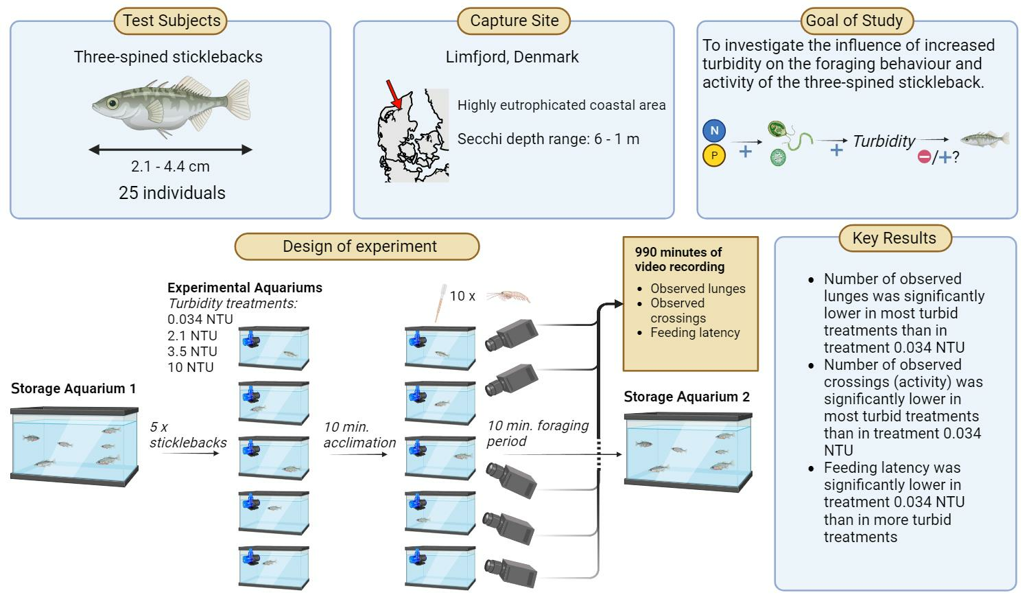
2.1. Sticklebacks for the Study

Sticklebacks used in the study were from an aquarium located in the North Sea Oceanarium (Hirtshals, Denmark). They were habituated in an aquarium set-up (simulating natural conditions) made by professional zookeepers around 2 months after being collected in the nearby Limfjord, the largest fjord system in Denmark and one of the most eutrophicated coastal areas in Denmark. Turbidity at the site of capture in spring was 1.5 ± 0.5 NTU (mean ± SE) and the closest measurements of Secchi depth in the Limfjord from the Danish Environmental Agency ranged from 6 m on the 5 January 2023 and 1 m on the 9 August 2023. The water in the storage aquarium was continuously recirculated and filtered by the facilities present at the North Sea Oceanarium. They were inspected daily and fed thawed Mysis sp. once a day before, during and after the experimental trials, with the exception of the day before each experimental trial. All individuals were in good condition before, during and after the study period.

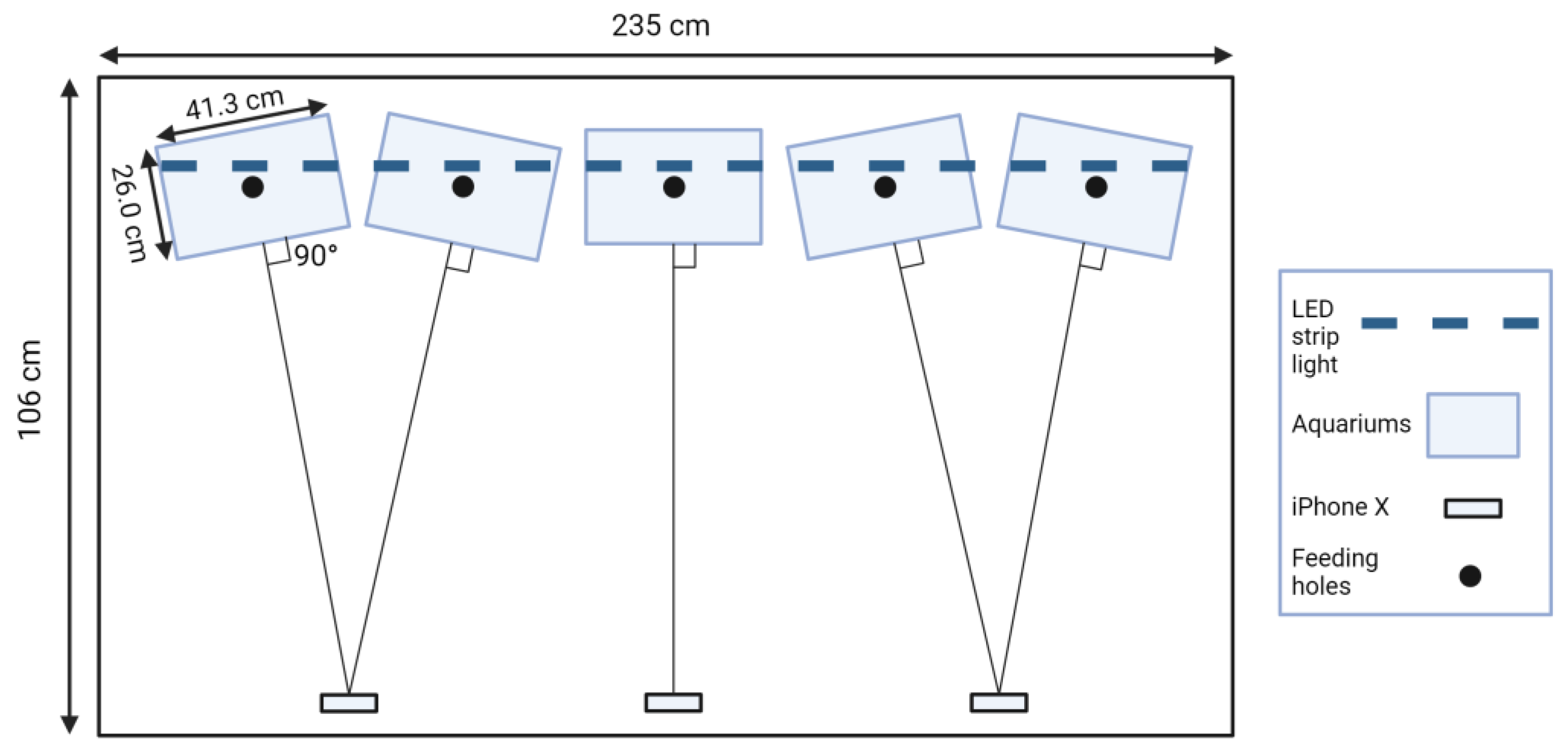
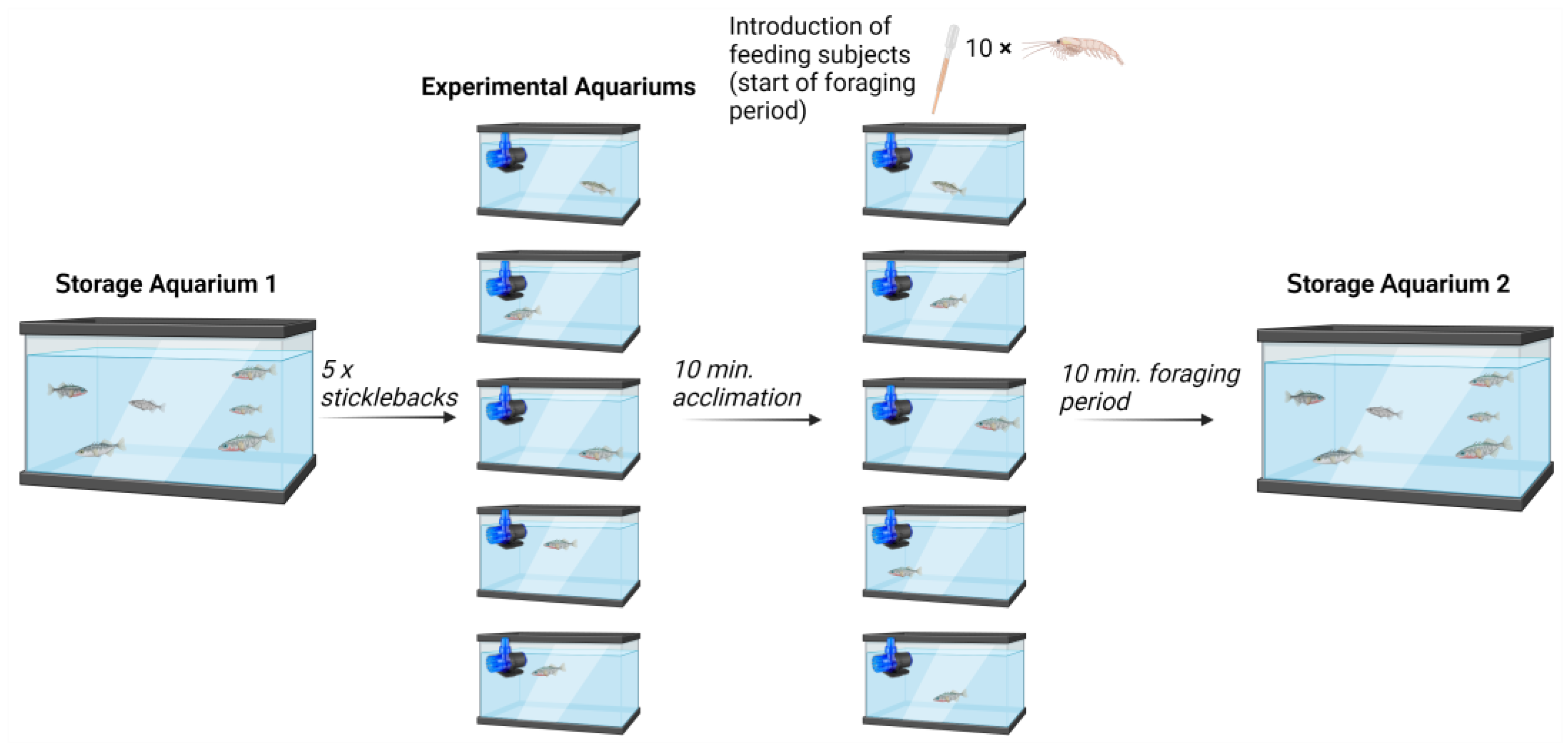
2.2. Design of Experimental Setup

The twenty-five individuals used in the study ranged (snout to caudal peduncle) from 2.1 to 4.4 cm with a size of 3.2 $\pm$ 0.12 cm (mean $\pm$ SE). Experiments were conducted in 21 L plastic aquariums with the dimensions 41.3 $\times$ 26 $\times$ 29.8 cm. The same 25 individuals were used in this study with the intent of minimising individual variation. This approach could potentially influence behaviour as the treatments are executed and/or the individuals are acclimated to the circumstances of the experiment. Consequently, the order of the execution of treatments with different turbidities was randomised with the purpose of controlling for potential stress or acclimation caused by the execution of the experiment. All individuals were stored in the same storage aquarium to ensure identical treatment between observation periods. The individuals were not tagged to avoid stress caused by handling and to minimise changes in behaviour from tagging. Therefore, the randomisation of the order of treatments for individual fish was not possible. The order in which the treatments were executed was (1) 0.034 NTU, (2) 3.5 NTU, (3) 2.1 NTU and (4) 10 NTU.

The aquariums used were placed in a closed wooden box to prevent visual disturbances from outside and prevent prediction of feeding events, and the experimental setup is shown in Figure 1. Video monitoring was performed using three iPhone Xs with a 1920 $\times$ 1080 pixel resolution and in automatic exposure mode. The focal length is 4 mm, and the camera sensor size is 1/3 inch approximately 8.5 mm.

The aquariums were oriented towards the iPhone Xs to minimise differences in refraction, which could interfere with the perceived position of the individuals. An LED strip light was installed directly over the aquariums to control the light source. All aquariums were very well and evenly illuminated. Pipettes with saltwater and ten thawed krill sp. were prepared before the start of the experiment. The wooden box had holes above each aquarium through which the feeding subjects were introduced to the aquariums (Figure 1).

Salinity in experimental aquariums was measured before the beginning of the experiment (

Table 1. Turbidity, temperature, and salinity in the experimental aquariums for each treatment (mean $\pm$ SE). “n” signifies sample size.

	0.034 NTU	2.1 NTU	3.5 NTU	10 NTU
Turbidity (NTU)	$0.034 \pm$ 0.026 (n= 10)	$2.1 \pm$ 0.15 (n = 10)	$3.5 \pm$ 0.057 (n = 10)	$10 \pm$ 0.48 (n = 10)
$\mathrm{Temperature} \mathrm{start} (°$C)	$9.1 \pm$ 0.037 (n = 5)	$9.6 \pm$ 0.025 (n = 5)	$8.9 \pm$ 0.037 (n = 5)	$9.6 \pm$ 0.020 (n = 5)
$\mathrm{Temperature} \mathrm{end} (°$C)	$12 \pm$ 0.037 (n = 5)	$12 \pm$ 0.025 (n = 5)	$11 \pm$ 0.020 (n = 5)	$12 \pm$ 0.020 (n = 5)
$\mathrm{Salinity} \left(\mathrm{‰}\right)$	30 (n = 1)	31 (n = 1)	31 (n = 1)	30 (n = 1)

). Temperatures were measured at the start and end of each treatment (Table 1) to assess potential behavioural responses to changes in temperature since this was not entirely controllable. The temperature increase between the start and end of each treatment is caused by heating from the surrounding facility.

Bentonite clay (hereafter referred to as clay) has been used in studies with similar experimental setups [13,21]. It is used to introduce turbidity to the water and is harmless to fish. Turbidity was measured using a turbidity meter (“Orion AQ3010”, Thermo Fisher Scientific, Waltham, Massachusetts, USA), and four mean turbidities were used in the experiment (0.034 (no clay added), 2.1, 3.5, and 10 NTU (Table 1)).

The effect of the different treatments is indicated in Figure 2. The clay was added to each aquarium 15 min before introducing the first test subjects. A circulation pump (“StreamMax Classic 2000”, OASE, Andover, UK) was necessary to keep the clay and the feeding subjects suspended, and it was placed close to the back wall and in the corner of quadrant II with the intent of freeing space in quadrant II. After experimentation, water samples were taken from all aquariums to measure turbidity and salinity (

Table 2. Overview of results for the variables observed crossings, feeding latency, observed lunges and proportion of time spent in the lower half of the aquarium (t_low) in each treatment. The sample size is indicated at the bottom of each column. The sample size is one less for all variables in the treatment with 0.034 NTU due to a failed recording. The sample size differed for the variable “feeding latency” because some test subjects did not feed during the experiment. Standard error, minimum value and maximum value are abbreviated as “SE”, “Min”, and “Max”, respectively.

0.034 NTU	Observed Crossings (n)	Feeding Latency (s)	Observed Lunges (n)	tlow
Mean	52	25	29	0.50
SE	7.0	11	3.9	0.064
Min	0	1	0	0
Max	138	268	76	0.96
Sample size (n)	24	23	24	24
2.1 NTU	Observed Crossings (n)	Feeding Latency (s)	Observed Lunges (n)	tlow
Mean	40	52	13	0.62
SE	6.2	13	2.2	0.059
Min	0	5	0	0.078
Max	113	252	46	1
Sample size (n)	25	23	25	25
3.5 NTU	Observed Crossings (n)	Feeding Latency (s)	Observed Lunges (n)	tlow
Mean	34	92	8.0	0.58
SE	5.6	27	1.9	0.070
Min	0	6	0	0.057
Max	93	435	37	1
Sample size (n)	25	20	25	25
10 NTU	Observed Crossings (n)	Feeding Latency (s)	Observed Lunges (n)	tlow
Mean	17	66	6.8	0.65
SE	3.8	20	1.5	0.067
Min	0	5	0	0
Max	85	368	25	1
Sample size (n)	25	20	25	25

).

Each turbidity treatment was performed separately over four experimental days, where the same 25 test subjects were used for all treatments. Because the experimental setup consisted of 5 experimental aquariums containing one test subject each at a time, an experimental day consisted of 5 sessions (Figure 3). The aquariums were labelled “1” to “5” for identification in video monitoring. The water in the experimental aquariums was not changed between runs. The sticklebacks were gently transferred individually from the storage aquarium to one of five experimental aquariums and acclimated for 10 min. After acclimation, 10 thawed krill were added to each aquarium, marking the start of the foraging period. The sticklebacks were given 10 min to forage, after which recording was stopped, and the fish were transported to a second storage aquarium (Figure 3). After each session, any remaining feeding subjects and potential fish waste were removed by a fine mesh net before the introduction of the following five sticklebacks.

2.3. Data and Statistical Analysis

Data were acquired from video recordings by visual evaluation of previously specified behaviours. The experimental aquariums were divided into four equally sized quadrants indicated in Figure 4. The defined behaviours were the total time spent in each quadrant, the total number of observed crossings between quadrants, the total number of observed lunges, feeding latency and the intervals of time in which the lunges were observed. Crossings are defined as when the test subjects moved from one quadrant to another, and the entirety of their body was inside the quadrant before the crossing was noted. This way of estimating activity ensures that highly active individuals in a single quadrant will not be regarded as highly active and that individuals who are oscillating between two quadrants will not have inflated activity. A lunge is defined as a clear and sudden acceleration towards a feeding subject. The total number of observed lunges is used as a measure of prey intake. Time intervals for lunges were estimated to assess whether lunges were evenly distributed over the 10 min course and whether this was different between treatments. The number of observed crossings is used to estimate boldness since crossings indicate activity.

The proportion of time spent in the lower half of the aquarium was calculated as follows:

$$t_{low}=\frac{t_{III}+t_{IV}}{600},$$

(1)

where $t_{low}$ is the proportion of time spent in the lower half of the aquarium, $t_{III}$ is seconds observed in quadrant III, $t_{IV}$ is seconds observed in quadrant IV, and 600 is the total experimental period in seconds. A low $t_{low}$ is indicative of high boldness since spending more time in the two upper quadrants is assumed to be related to bold behaviour.

The statistical analysis was carried out in R-studio and Microsoft Excel with significance levels of * p < 0.05; ** p < 0.01; *** p < 0.001. The total number of observed crossings, the total number of observed lunges, the proportion of time spent in the lower half of the aquarium and the number of observed lunges within the 60 s intervals were tested for normality and variance homogeneity with a Shapiro–Wilk test and Bartlett’s test, respectively. All dependent variables were not normally distributed and had no homogeneity in variance, so all following statistical analysis was performed with non-parametric tests. Despite the data not being independent, as the same 25 individuals were used for all treatments, differences in dependent variables between treatments were tested with the Kruskal–Wallis Rank Sum test. This was conducted because the experimental design entailed that individuals were unidentifiable, and hence, tests with repeated measures were impossible. In the case of significant differences between treatments, Dunn’s test was used post hoc [22]. Correlation between dependent variables and the size of individuals was tested with Spearman’s Rank correlation test, and differences in dependent variables between individuals used at the start and end of each experimental day were tested with the Wilcoxon Signed Rank test. Dunn’s tests were adjusted with Bonferroni correction [23].

For the feeding latency and its behavioural instability, the median, variance (estimated by the median absolute deviation), kurtosis and asymmetry (estimated by the skewness) were calculated for all the turbidity treatments. The median absolute deviations were tested for differences between the turbidity treatments with a Mann–Whitney U-test. Differences in kurtosis and asymmetry (skewness) were tested by bootstrapping (999 bootstrap) and estimating the 95% confidence intervals.

3. Results

3.1. Sample Summary

A total of 25 sticklebacks were recorded at each turbidity level. However, one recording from the treatment with a turbidity of 0.034 NTU failed. Consequently, the total number of observations was 99, resulting in a total of 990 min of footage, as the foraging period was 10 min. An overview of the results is provided in Table 2.

3.2. The Influence of Change in Temperature on Foraging Behaviour and Activity

During each experimental day, the water temperature in the aquariums increased by around 2 degrees (Table 1). Kruskal–Wallis tests showed that the size and temperature were not statistically significantly (hereafter referred to as “significant”) different between the four treatments, and therefore, the turbidities have been pooled for the following Spearman’s Rank correlation test and Wilcoxon Signed Rank test (p > 0.05, n = 99). Spearman’s Rank Correlation test showed no significant correlation between either observed lunges or number of crossings and size (p > 0.05, n = 99), and the Wilcoxon Signed Rank test showed that there was no significant difference in either observed lunges or number of crossings between the individuals used at the start and end of experimental days (p > 0.05, n = 38).

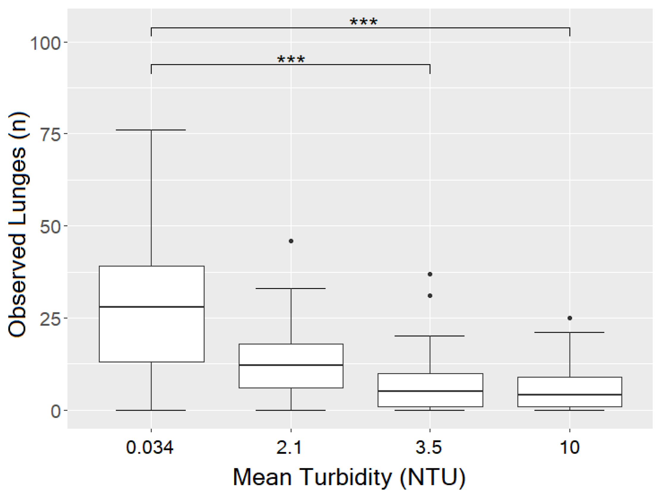
3.3. Influence of Turbidity on Observed Lunges

Fewer lunges by the sticklebacks were observed with increasing turbidity (Figure 5). A Kruskal–Wallis Rank Sum test indicated a significant difference in observed lunges between the treatments with different turbidities (p < 0.001, n = 99). Dunn’s test indicated significantly fewer observed lunges between the treatment with a turbidity of 0.034 NTU and the two treatments with the highest turbidities (p < 0.001, n = 49 for both tests). Hence, there were significantly fewer observed lunges between the treatment executed on the first experimental day (0.034 NTU) and the treatments executed on the second and last experimental days (3.5 and 10 NTU, respectively). The number of observed lunges was not significantly lower for the treatment executed on the second experimental day (3.5 NTU) than for the treatment executed on the third experimental day (2.1 NTU).

The number of observed lunges in different intervals of 60 s for all treatments is indicated in Figure 6. Kruskal–Wallis Rank Sum tests showed that the number of observed lunges differed significantly between some of the turbidities in all the 60 s intervals (p < 0.05, n = 25, n = 24 for treatment 0.03 NTU). Multiple Dunn’s tests showed that the number of observed lunges in the first 60 s differed significantly from some of the later intervals in all treatments. The number of observed lunges in the first 60 s differed significantly between the treatments with turbidities of 0.034 NTU and both 3.5 NTU (p < 0.001, n = 49) and 10 NTU (p < 0.01, n = 49). The number of observed lunges in the last 60 s differed between the treatment with a turbidity of 0.034 NTU and all other treatments (p < 0.01, n = 49 for all tests).

A higher feeding latency was observed with increasing turbidity (Figure 7). A Kruskal–Wallis Rank Sum test indicated a significant difference between the treatments with different turbidities (p < 0.01, n = 99). A Dunn’s test indicated a significantly lower feeding latency of the least turbid treatment relative to all other treatments (0.034 NTU and 2.1 NTU p < 0.01; 0.034 NTU and 3.5 NTU p < 0.05; 0.034 NTU and 10 NTU p < 0.01, n = 49 for all tests). The feeding latency was not significantly higher for the treatments executed on the second experimental day (3.5 NTU) than the treatment executed on the third experimental day (2.1 NTU). The results from Dunn’s tests are provided in Appendix A (

Table A1. Dunn’s test for differences in observed lunges within 60 s intervals between turbidity treatments.

Interval [s]	0.03–2.15 NTU	0.03–3.51 NTU	0.03–10.12 NTU	2.15–3.51 NTU	2.15–10.12 NTU	3.51–10.12 NTU
0–59	p > 0.05	p < 0.001	p < 0.01	p > 0.05	p > 0.05	p > 0.05
60–119	p < 0.05	p < 0.001	p < 0.001	p > 0.05	p > 0.05	p > 0.05
120–179	p > 0.05	p < 0.001	p < 0.01	p > 0.05	p > 0.05	p > 0.05
180–239	p > 0.05	p < 0.01	p < 0.001	p > 0.05	p > 0.05	p > 0.05
240–299	p > 0.05	p < 0.05	p < 0.01	p > 0.05	p > 0.05	p > 0.05
300–359	p > 0.05	p < 0.01	p < 0.01	p > 0.05	p > 0.05	p > 0.05
360–419	p > 0.05	p < 0.05	p < 0.01	p > 0.05	p > 0.05	p > 0.05
420–479	p > 0.05	p > 0.05	p < 0.05	p > 0.05	p > 0.05	p > 0.05
480–539	p < 0.01	p < 0.001	p < 0.001	p > 0.05	p > 0.05	p > 0.05
540–600	p < 0.01	p < 0.001	p < 0.001	p > 0.05	p > 0.05	p > 0.05

and

Table A2. Dunn’s test for differences within treatments between 60 s intervals.

Interval [s]	0.03 NTU	2.15 NTU	3.51 NTU	10.12 NTU
0–59 and 240–299	p < 0.05	p > 0.05	p > 0.05	p > 0.05
0–59 and 360–419	p < 0.05	p > 0.05	p > 0.05	p > 0.05
0–59 and 420–479	p < 0.001	p > 0.05	p > 0.05	p > 0.05
0–59 and 480–539	p < 0.05	p > 0.05	p > 0.05	p < 0.01
0–59 and 540–600	p < 0.05	p < 0.01	p > 0.05	p < 0.05
60–119 and 420–479	p < 0.05	p > 0.05	p > 0.05	p > 0.05

).

3.4. Behavioural Instability

The behavioural instability of feeding latency estimated by the median absolute deviation showed a significant increase in the instability with increased turbidity ((0.034 NTU; median = 5, n = 24) < (2.1 NTU; median = 21, n = 25) *** and (0.034 NTU; median = 5, n = 24) < (3.5 NTU; median = 21.5, n = 25) ***), whereas for the highest level of turbidity (10 NTU; median = 11.5, n = 25), no significant differences were found between the other treatments (p > 0.05) (Figure 8).

The behavioural instability of feeding latency estimated by the kurtosis was significantly higher (leptokurtic) at the lowest turbidity compared to all three higher levels of turbidity, which showed a more platykurtic distribution: (0.034 NTU; kurtosis = 21.16, n = 24) > (2.1 NTU; kurtosis = 4.21, n = 25)* and (0.034 NTU; kurtosis = 21.16, n = 24) > (3.5 NTU; kurtosis = 2.78, n = 25) * and (0.034 NTU; kurtosis = 21.16, n = 24) > (10 NTU; kurtosis = 6.36, n = 25) *. No other significant differences in kurtosis were found between the turbidity treatments NTU 2.1, 3.5 and 10 (all p > 0.05) (Figure 8).

The behavioural instability of feeding latency estimated by the asymmetry (skewness) was significantly higher (skewed on the right) at the lowest turbidity compared to all three higher levels of turbidity, which showed a more symmetric (less skewed) distribution: (0.034 NTU; skewness = 4.53, n = 24) > (2.1 NTU; skewness = 2.16, n = 25) * and (0.034 NTU; skewness = 4.53, n = 24) > (3.5 NTU; skewness = 1.87, n = 25) * and (0.034 NTU; skewness = 4.53, n = 24) > (10 NTU; skewness = 2.44, n = 25) *. No other significant differences in kurtosis were found between the turbidity treatments NTU 2.1, 3.5 and 10 (all p > 0.05) (Figure 8).

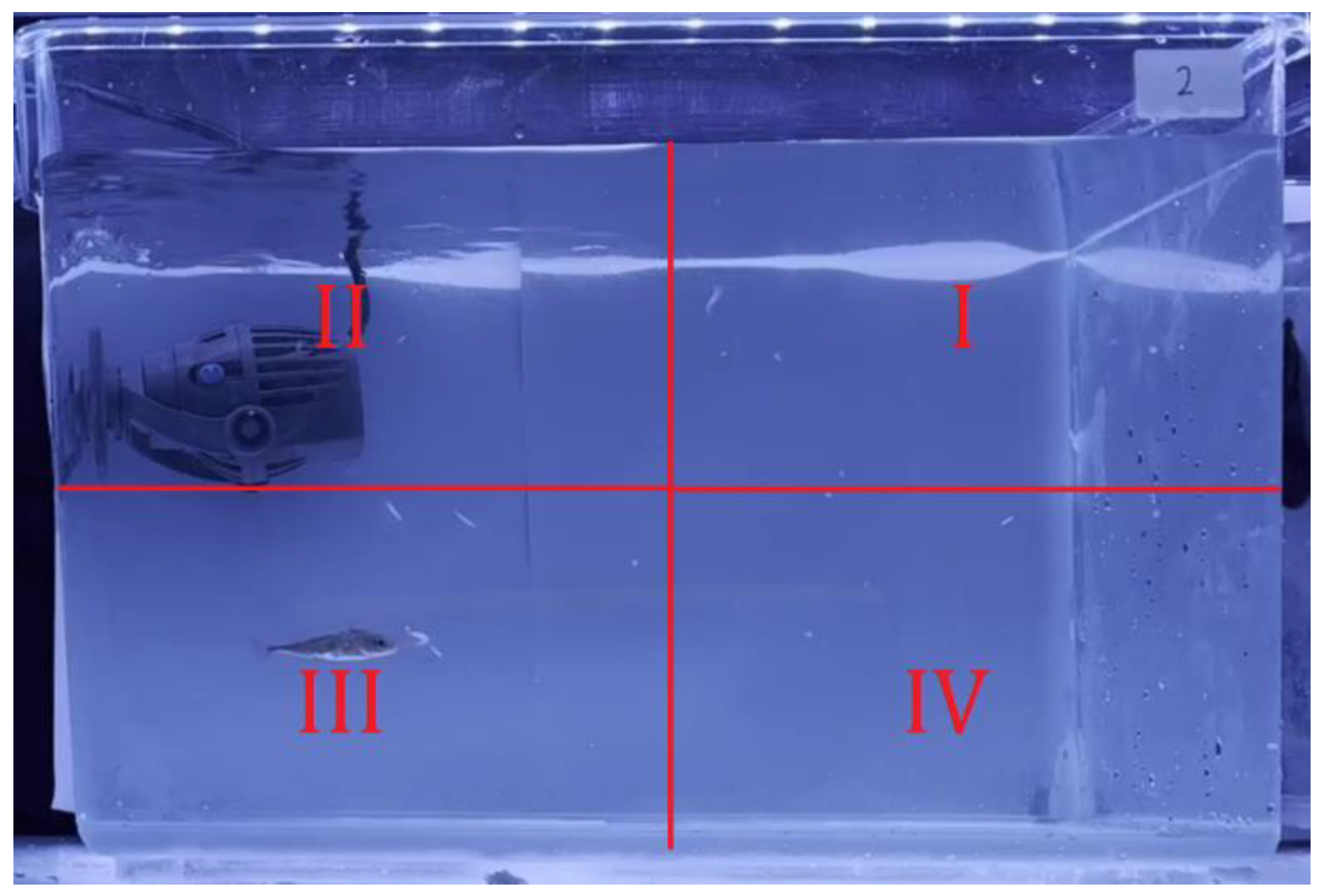
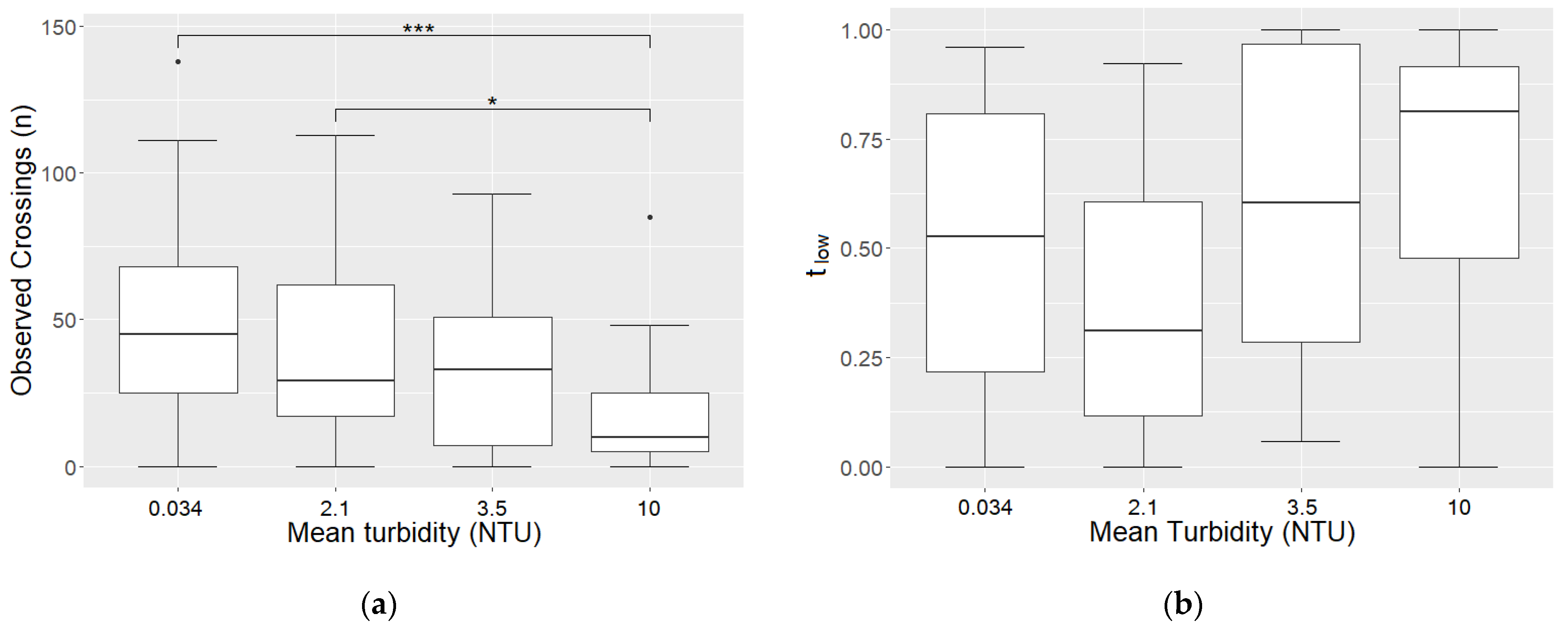
3.5. The Influence of Turbidity on Activity and Time Spent in the Lower Half of Aquarium

The sticklebacks moved less between quadrants when turbidity was increased (Figure 9a). A Kruskal–Wallis test indicated a significant difference in observed crossings between the treatments with different turbidities (p < 0.01, n = 99). A Dunn’s test indicated significant differences in the number of observed crossings between both treatments with the lowest turbidities and the treatment with the highest turbidity (p < 0.001, n = 99). The number of observed crossings was not significantly lower for the treatment executed on the second experimental day than for the treatment executed on the third experimental day. A Kruskal–Wallis Rank Sum test showed that there was no significant difference in the proportion of time spent in the lower half of the aquarium (t_low) between the treatments (p > 0.05, n = 99) (Figure 9b).

4. Discussion

4.1. Methodology

All individuals were stored in the same aquarium to ensure identical treatments between observation periods and to heighten natural behaviour, and were not tagged to avoid invasive treatments. Consequently, this design does not benefit from being able to identify fish individually and makes it impossible to randomise the order of execution of treatments for each individual fish. This was partially accommodated by treating all fish with the same turbidity each day and randomising the order of these days, but since no dependent variables were significantly different between the treatments executed on the second and third experimental days, it is impossible to say with certainty that the effect on dependent variables is from turbidity and not from individuals acclimating to the circumstances of the experiment. This could be accommodated by including more treatments with a randomised order of execution, as it would be clearer whether the turbidity of treatments or the order of execution of treatments is the cause of the effect. However, both the number of observed lunges and the number of observed crossings were not significantly different between any two treatments executed on experimental days separated by more than one day except for between the two treatments with the lowest and highest turbidity, which were executed on the first and last day, respectively, which indicates that turbidity is more likely the cause of the effect.

4.2. The Influence of Temperature and Size

Changes in temperature from the transfer between the storage and experimental aquarium did not influence the foraging behaviour and activity of sticklebacks since no significant difference in observed lunges or number of crossings was observed between individuals used at the start and end of each experimental day. The lack of correlation of size with observed lunges or number of observed crossings indicates that when sticklebacks are isolated, size in the range of the test subjects has no effect on their foraging behaviour and activity.

Since the amount of odour cues would be expected to increase during each experimental day, like the temperature, these cues are implicitly shown to have no significant influence on the foraging behaviour and activity of the sticklebacks.

Although no significant correlation between size and observed lunges or number of observed crossings was found in this study, greater fish size leads to higher energy requirements [24]. It was, therefore, expected that more lunges would be observed for the larger test subjects and that the larger test subjects would be more active. The results concerning observed lunges were not in accordance with a study by Jolles et al. [24], who used the number of prey items eaten instead of observed lunges as a measure of food intake [24]. Jolles et al. [24] used sticklebacks from a river (UK) to investigate boldness and food intake in individuals of different sizes (3.06–5.25 cm, snout to caudal peduncle). Boldness was estimated as time spent outside a site with plant cover in test aquariums, and the fish were fed Chironomus sp. during the experiment. They found that boldness did not correlate with the length of the fish. However, they observed larger individuals to have a higher food intake [24]. This difference in results could be explained by the fact that the test subjects in the study by Jolles et al. [24] were caught in a river and were thereby a different ecotype than the test subjects in this study. Another explanation could be the difference in feeding subjects. Chironomus sp. are red, whereas the feeding subjects in this study had little colour. This could influence the foraging behaviour as sticklebacks use prey colouration to detect and capture prey [13].

4.3. The Influence of Turbidity on Foraging Behaviour

The treatment with a turbidity of 0.034 NTU had a significantly higher number of observed lunges than the treatments with the highest turbidities and no significant difference in the number of observed lunges compared to the treatment with a turbidity of 2.1 NTU. The treatment with a turbidity of 2.1 NTU was performed on the third experimental day and did not differ significantly in the number of observed lunges compared to the treatment executed on the first experimental day (0.034 NTU). These treatments, therefore, are separated by a whole experimental day; it is less likely that this result is caused by the individuals acclimating to the circumstances of the experiment. Hence, the difference in number of observed lunges is more likely caused by the turbidity.

This is in accordance with a result by Sohel et al. [25] who found a clear decreasing trend in the number of prey eaten with increasing turbidity [25]. Compared to a study by Quesenberry et al. [13], the foraging behaviour of sticklebacks in this study appeared much more sensitive to increased turbidity [13]. Quesenberry et al. [13] did not find any significant difference in the number of observed feeding lunges between different mean turbidities (ANOVA p > 0.05), even though many of their treatments were far more turbid than those in this study. The mean turbidities of the treatments in the study by Quesenberry et al. [13] were 5–10 NTU, 20–30 NTU, 40–60 NTU, and 60–80 NTU. Differences in results might be caused by differences in adaptation to turbidity between the test subjects of the two studies as it is well known that some behaviours of sticklebacks are genetically correlated and that genomes vary between separated populations of three-spined sticklebacks [26,27]. This is supported by the results from a study by Webster et al. [28], where the number of prey items consumed differed between test subjects caught at different sites with different ranges of turbidity [28]. Differences in results between the study by Quesenberry et al. [13] and this study could also be caused by the acclimation to different turbidities, as none of the studies have used bred fish from different environments as test subjects. Whether the difference in observed lunges between test subjects caught from areas with varying turbidity ranges is due to adaptation or acclimation could be examined. The study by Quesenberry et al. [13] found a generally higher number of observed feeding lunges independent of turbidity, which could be explained by the higher temperature in their experimental aquarium (10 to 17 $°$C) as well as at their site of capture (15 $\pm$ 3 $°$C) as a study by Lefébure et al. [29] found that the attack rate of sticklebacks was significantly influenced by temperature [29].

For the lowest turbidities, it appears that the number of observed lunges in the first two 60 s intervals is what determines the lowered number of observed lunges in the following intervals, as the many lunges, in the beginning, cause the number of krill in the following intervals to be lowered, and therefore the number of opportunities for lunges to be lowered. In the treatments with higher turbidities, the number of observed lunges in the first 60 s intervals is much lower and has less influence on the number of lunges in the following intervals. However, it seems that the observed lunges were similarly distributed between the intervals of 60 s between all four turbidities, with more observed lunges in the first two intervals of 60 s compared to the following intervals.

The treatment with a turbidity of 10 NTU had a significantly lower feeding latency than the treatments with the lowest turbidities and no significant difference in feeding latency compared to the treatment with a turbidity of 3.5 NTU. The treatment with a turbidity of 3.5 NTU was executed on the second experimental day and did not differ significantly in feeding latency compared to the treatment executed on the fourth experimental day (10 NTU). These treatments are therefore separated by a whole experimental day, so it is less likely that this result is caused by the individuals acclimating to the circumstances of the experiment and hence, the difference in feeding latency is more likely caused by the turbidity.

This is not in accordance with a study by Vollset and Bailey [21], where no significant decrease in feeding latency with increasing turbidity was observed [21]. However, their site of capture was an estuary (USA), where the test subjects were frequently exposed to periods with higher turbidities. The absence of observed influence of increased turbidity on feeding latency in their study might be caused by the higher turbidities at their capture site [21].

4.4. The Influence of Turbidity on Activity and Vertical Placement

Increasing turbidity had no significant effect on the proportion of time that sticklebacks spent in the lower half of the aquarium. The test subjects were not exposed to any predators before and during the experiment, which could explain why no effect on vertical positioning was observed. Turbidity seems to instead have an influence on the activity of the fish, which is more clearly relevant for the evasion of predators, as cautious movement could lead to a lowered risk of predation when turbidity is increased. In this study, the number of observed crossings between quadrants was used as an indicator of activity. The treatments with the lowest turbidities had a significantly higher number of observed crossings than the treatment with a turbidity of 10 NTU, and no significantly different number of observed crossings compared to the treatment with a turbidity of 3.5 NTU. The treatment with a turbidity of 3.5 NTU was performed on the second experimental day and did not differ significantly in the number of observed crossings compared to the treatment executed on the fourth experimental day (10 NTU). These treatments, therefore, are separated by a whole experimental day; it is less likely that this result is caused by the individuals acclimating to the circumstances of the experiment. Hence, the difference in number of observed crossings is likely caused by the turbidity.

The significantly reduced activity in turbid environments can be interpreted as increased cautious behaviour because a reduced visual field makes predator evasion more difficult. In a study by Ajemian et al. [30], significantly more sticklebacks were observed sheltering in vegetated habitats at 13–15 $\pm$ 0.5 NTU and 7–9 $\pm$ 0.5 NTU than treatments with 2–3 $\pm$ 0.5 NTU, which indicates that sticklebacks show more cautious behaviour when in turbid environments [30]. However, some studies suppose that high turbidity in itself acts as a hide [31]. Using turbid waters as a hide is especially relevant when vegetation and natural hides are not present. A study by Engström-Öst et al. [31] observed that sticklebacks chose areas with high turbidity caused by high concentrations of cyanobacteria when exposed to chemical predator signals [31]. It, therefore, seems that the influence of turbidity on the boldness of sticklebacks depends on the presence and nature of the available hides.

4.5. Behavioural Instability

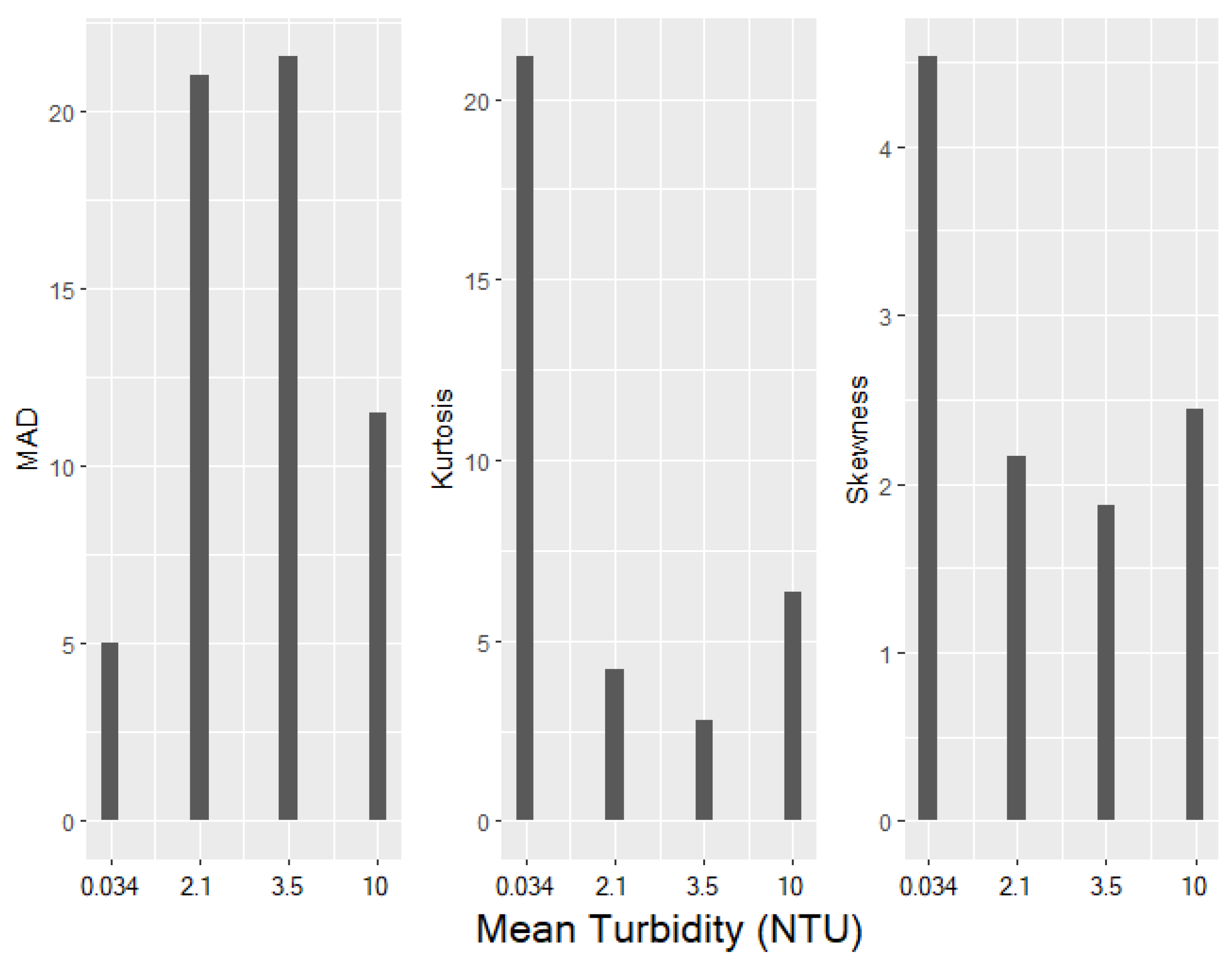
The behavioural instability of feeding latency has shown a clear trend for all the estimates:

(a)

The median absolute deviation increases with increasing levels of turbidity, with the exception of the highest turbidity (NTU 10), indicating a clear increase in the variability of feeding latency, which can be translated into a higher level of unpredictability in the time interval between a stimulus or opportunity for feeding and the initiation of feeding behaviour in an animal.

(b)

The reduction of kurtosis at the higher level of turbidity supports the increase in the median absolute deviation at the higher level of turbidity, as a reduction in kurtosis flattens the distribution curve and expands the tails of the distribution.

(c)

The reduction in the symmetry (skewness) observed at a higher level of turbidity indicates that at a low level of turbidity, the variation (of the time interval between a stimulus or opportunity for feeding and the initiation of feeding behaviour) is due to several long intervals of latency, which increase the tailness of the distribution on the right side. At higher levels of turbidity, the distributions tend to become more symmetric, which indicates that the increased variation observed at higher turbidity is not mainly due to higher skewness but is due to a flattening of the distribution and an increase of tailness on both sides of the distribution.

4.6. Eutrophication in Coastal Environments

The three-spined stickleback is opportunistic and capable of adapting to changes in environmental conditions and is, therefore, not the most sensitive fish species to changes in turbidity [16]. However, other fish species that are visual predators might be affected by eutrophication in coastal environments.

Eutrophication is a global problem in coastal areas, and coastal areas in Denmark are highly affected. Our experimental sticklebacks originated from the highly eutrophicated Limfjord, the largest Danish fjord system. Therefore, the individuals would be expected to be less influenced by turbidity than sticklebacks from less turbid environments. According to a study by Tomczak et al. [16], the regime shift in the Limfjord in the 1990s was caused by top-down influences, primarily fishery, and bottom-up influences from increased nitrogen and phosphorous loadings from agricultural activity [16]. Since the early 1900s, nutrient loadings in the Limfjord have increased sixfold [32].

The reduction in loadings since the mid-1980s has not resulted in any noticeable effects on the ecosystems of the Limfjord [16] and most of the Danish fjord systems and coastal areas. This is necessary to achieve ‘good environmental status’, which EU members are required to meet according to the water framework directive [33]. Eutrophication and, hence, turbidity are likely to occur in the following decades, and opportunistic species like the stickleback may be favoured. However, studies on the species’ ability to acclimate to increasing turbidity, hence studies with much longer exposures to turbidity, are required to estimate the potential influence of eutrophication on stickleback populations.

5. Conclusions

The foraging behaviour and activity of the test subjects were significantly affected by turbidity in an experimental setup without social interactions, predation, and natural surroundings. These results indicate that populations of three-spined sticklebacks are altered when coastal environments become more turbid. Still, research into the effects of turbidity on populations of three-spined sticklebacks is required. These results are in partial accordance with results from studies that used different experimental setups where less clear effects from turbidity were found. Habitat-specific differences in behavioural patterns between different populations of three-spined sticklebacks could explain the incongruence in results between different studies, and it is speculated whether habitat-specific differences in behaviour are indicative of a plastic response or an evolutionary response.

The increased behavioural instability observed with reduced visibility suggests that increasing unpredictability of the behaviour could have an adaptative value, which could have consequences on individual fitness. However, to be adaptative, a behavioural trait should have a certain degree of inheritance, suggesting a heritability of personality traits. If behavioural instability does not have a hereditary component, it will not have evolutionary significance and is a purely plastic response. Several experiments could be designed to estimate the potential heritability of behavioural instability; for example, personality experiments where instead of only focusing on the quantification of a behavioural response, components like variation, symmetry, and kurtosis should be considered [19,20,34].

Increased turbidity is a common consequence of eutrophication globally. This study has investigated the influence of a bottom-up impact from anthropogenic activity on the foraging behaviour of a small opportunistic fish species and found a significant effect. Larger, more sensitive, and economically relevant species are also impacted by eutrophication in relation to their foraging behaviour. Our results emphasise the importance of reducing nutrient loadings to ensure good ecological status as part of reaching the objectives included in the EU water framework directive.

References

1. Wollschläger, J.; Neale, P.J.; North, R.L.; Striebel, M.; Zielinski, O. Editorial: Climate Change and Light in Aquatic Ecosystems: Variability and Ecological Consequences. Front. Mar. Sci. 2021, 8, 688712. [Google Scholar] [CrossRef]
2. Gorokhovich, Y. Turbidity. In Encyclopedia of Estuaries; Kennish, M.J., Ed.; Springer: Dordrecht, Netherlands, 2016; pp. 720–721. [Google Scholar]
3. Abrams, P.A. Optimal Traits When There are Several Costs: The Interaction of Mortality and Energy Costs in Determining Foraging Behavior. Behav. Ecol. 1993, 4, 246–259. [Google Scholar] [CrossRef]
4. Vlieger, L.; Candolin, U. How Not to Be Seen: Does Eutrophication Influence Three-Spined Stickleback Gasterosteus aculeatus Sneaking Behaviour? J. Fish Biol. 2009, 75, 2163–2174. [Google Scholar] [CrossRef]
5. Fischer, S.; Frommen, J.G. Eutrophication Alters Social Preferences in Three-Spined Sticklebacks (Gasterosteus aculeatus). Behav. Ecol. Sociobiol. 2013, 67, 293–299. [Google Scholar] [CrossRef]
6. Paerl, H.W. Controlling Eutrophication Along the Freshwater-Marine Continuum: Dual Nutrient (N and P) Reductions are Essential. Estuaries Coasts 2009, 32, 593–601. [Google Scholar] [CrossRef]
7. McCrackin, M.L.; Jones, H.P.; Jones, P.C.; Moreno-Mateos, D. Recovery of Lakes and Coastal Marine Ecosystems from Eutrophication: A Global Meta-Analysis. Limnol. Oceanogr. 2017, 62, 507–518. [Google Scholar] [CrossRef]
8. Riemann, B.; Carstensen, J.; Dahl, K.; Fossing, H.; Hansen, J.W.; Jakobsen, H.H.; Josefson, A.B.; Krause-Jensen, D.; Markager, S.; Stæhr, P.A.; et al. Recovery of Danish Coastal Ecosystems After Reductions in Nutrient Loading: A Holistic Ecosystem Approach. Estuaries Coasts 2016, 39, 82–97. [Google Scholar] [CrossRef]
9. Marin-Diaz, B.; Bouma, T.J.; Infantes, E. Role of Eelgrass on Bed-Load Transport and Sediment Resuspension under Oscillatory Flow. Limnol. Oceanogr. 2020, 65, 426–436. [Google Scholar] [CrossRef]
10. Ahnelt, H.; Ramler, D.; Madsen, M.Ø.; Jensen, L.F.; Windhager, S. Diversity and Sexual Dimorphism in the Head Lateral Line System in North Sea Populations of Threespine Sticklebacks, Gasterosteus aculeatus (Teleostei: Gasterosteidae). Zoomorphology 2021, 140, 103–117. [Google Scholar] [CrossRef]
11. Barber, I. Sticklebacks as Model Hosts in Ecological and Evolutionary Parasitology. Trends Parasitol. 2013, 29, 556–566. [Google Scholar] [CrossRef] [PubMed]
12. Spence, R.; Wootton, R.J.; Barber, I.; Przybylski, M.; Smith, C. Ecological Causes of Morphological Evolution in the Three-Spined Stickleback. Ecol. Evol. 2013, 3, 1717–1726. [Google Scholar] [CrossRef]
13. Quesenberry, N.J.; Allen, P.J.; Cech, J.J., Jr. The Influence of Turbidity on Three-Spined Stickleback Foraging. J. Fish Biol. 2007, 70, 965–972. [Google Scholar] [CrossRef]
14. Bretzel, J.B.; Geist, J.; Gugele, S.M.; Baer, J.; Brinker, A. Feeding Ecology of Invasive Three-Spined Stickleback (Gasterosteus aculeatus) in Relation to Native Juvenile Eurasian Perch (Perca fluviatilis) in the Pelagic Zone of Upper Lake Constance. Front. Environ. Sci. 2021, 9, 670125. [Google Scholar] [CrossRef]
15. Olin, A.B.; Olsson, J.; Eklöf, J.S.; Eriksson, B.K.; Kaljuste, O.; Briekmane, L.; Bergström, U.; Ojaveer, H. Increases of Opportunistic Species in Response to Ecosystem Change: The Case of the Baltic Sea Three-Spined Stickleback. ICES J. Mar. Sci. 2022, 79, 1419–1434. [Google Scholar] [CrossRef]
16. Tomczak, M.; Dinesen, G.E.; Hoffman, E.; Maar, M.; Støttrup, J.G. Integrated Trend Assessment of Ecosystem Changes in the Limfjord (Denmark): Evidence of a Recent Regime Shift? Estuar. Coast. Shelf Sci. 2013, 117, 178–187. [Google Scholar] [CrossRef]
17. Sohel, S.; Lindström, K. Algal Turbidity Reduces Risk Assessment Ability of the Three-Spined Stickleback. Ethology 2015, 121, 548–555. [Google Scholar] [CrossRef]
18. Pertoldi, C.; Bahrndorff, S.; Novicic, Z.K.; Rohde, P.D. The Novel Concept of “Behavioural Instability” and Its Potential Applications. Symmetry 2016, 8, 135. [Google Scholar] [CrossRef]
19. Linder, A.C.; Lyhne, H.; Laubek, B.; Bruhn, D.; Pertoldi, C. Modeling Species-Specific Collision Risk of Birds with Wind Turbines: A Behavioral Approach. Symmetry 2022, 14, 2493. [Google Scholar] [CrossRef]
20. Linder, A.C.; Lyhne, H.; Laubek, B.; Bruhn, D.; Pertoldi, C. Quantifying Raptors’ Flight Behavior to Assess Collision Risk and Avoidance Behavior to Wind Turbines. Symmetry 2022, 13, 2245. [Google Scholar] [CrossRef]
21. Vollset, K.W.; Bailey, K.M. Interplay of Individual Interactions and Turbidity Affects the Functional Response of Three-Spined Sticklebacks Gasterosteus aculeatus. J. Fish Biol. 2011, 78, 1954–1964. [Google Scholar] [CrossRef] [PubMed]
22. Zar, J.H. Biostatistical Analysis, 2nd ed.; Prentice Hall: Englewood Cliffs, NJ, USA, 1984. [Google Scholar]
23. Rice, W.R. Analyzing Tables of Statistical Tests. Evolution 1989, 43, 223–225. [Google Scholar] [CrossRef]
24. Jolles, J.W.; Manica, A.; Boogert, N.J. Food Intake Rates of Inactive Fish are Positively Linked to Boldness in Three-Spined Sticklebacks Gasterosteus aculeatus. J. Fish Biol. 2016, 88, 1661–1668. [Google Scholar] [CrossRef]
25. Sohel, S.; Mattila, J.; Lindström, K. Effects of Turbidity on Prey Choice of Three-Spined Stickleback Gasterosteus aculeatus. Mar. Ecol. 2017, 566, 159–167. [Google Scholar] [CrossRef]
26. Dingemanse, N.J.; Barber, I.; Dochtermann, N.A. Non-Consumptive Effects of Predation: Does Perceived Risk Strengthen the Genetic Integration of Behaviour and Morphology in Stickleback? Ecol. Lett. 2020, 23, 107–118. [Google Scholar] [CrossRef]
27. FitzGerald, G.J.; Wootton, R.J. Behavioural Ecology of Sticklebacks. In The Behaviour of Teleost Fishes; Pitcher, T.J., Ed.; Springer: Boston, MA, USA, 1986; pp. 409–432. [Google Scholar]
28. Webster, M.M.; Atton, N.; Ward, A.J.W.; Hart, P.J.B. Turbidity and Foraging Rate in Threespine Sticklebacks: The Importance of Visual and Chemical Prey Cues. Behaviour 2007, 144, 1347–1360. [Google Scholar]
29. Lefébure, R.; Larsson, S.; Byström, P. Temperature and Size-Dependent Attack Rates of the Three-Spined Stickleback (Gasterosteus aculeatus); Are Sticklebacks in the Baltic Sea Resource-Limited? J. Exp. Mar. Biol. Ecol. 2014, 451, 82–90. [Google Scholar] [CrossRef]
30. Ajemian, M.J.; Sohel, S.; Mattila, J. Effects of Turbidity and Habitat Complexity on Antipredator Behavior of Three-Spined Sticklebacks (Gasterosteus aculeatus): Antipredator Behavior in Sticklebacks. Environ. Biol. Fishes 2015, 98, 45–55. [Google Scholar] [CrossRef]
31. Engström-Öst, J.; Karjalainen, M.; Viitasalo, M. Feeding and Refuge Use by Small Fish in the Presence of Cyanobacteria Blooms. Environ. Biol. Fishes 2006, 76, 109–117. [Google Scholar] [CrossRef]
32. Dinesen, G.E.; Timmermann, K.; Roth, E.; Markager, S.; Ravn-Jonsen, L.; Hjorth, M.; Holmer, M.; Støttrup, J.G. Mussel Production and Water Framework Directive Targets in the Limfjord, Denmark: An Integrated Assessment for Use in System-Based Management. Ecol. Soc. 2011, 16, 26. [Google Scholar] [CrossRef]
33. Markager, S.; Storm, L.M.; Stedmon, C.A. Limfjordens Miljøtilstand 1985 til 2003. Sammenhæng Mellem Næringsstoftilførsler, Klima og Hydrografi Belyst ved Hjælp af Empiriske Modeller; Report 577; National Environmental Research Institute, Aarhus University: Aarhus, Denmark, 2006. [Google Scholar]
34. Linder, A.C.; Gottschalk, A.; Lyhne, H.; Langbak, M.G.; Jensen, T.H.; Pertoldi, C. Using Behavioral Instability to Investigate Behavioral Reaction Norms in Captive Animals: Theoretical Implications and Future Perspectives. Symmetry 2020, 12, 603. [Google Scholar] [CrossRef]
Figure 1. Arrangement of aquariums, LED strip light, iPhone Xs and feeding holes within the wooden box. The dimensions of the aquariums are shown at the leftmost aquarium. The diagram was created with BioRender.com accessed on the 15 December 2023.
Fishes 08 00609 g001
Figure 2. Experimental setup, showing one of the five aquariums used in four treatments with different turbidities. The photographs are captured from the same direction as the video recordings, and the aquarium is oriented with the largest and widest plane facing towards the camera. Turbidity of the treatments was measured in NTU, which is a unit used in quantifying turbidity and is a measure of the amount of light that is scattered and absorbed by suspended particles. Circulation pumps and test subjects are present in the aquarium. The second aquarium in the box has been used for visualisation, explaining the number “2” in the upper right corner.
Fishes 08 00609 g002
Figure 3. Diagram showing the simplified presentation of the procedure. Five test subjects were caught from a storage aquarium and introduced to each experimental aquarium. The test subjects were acclimated for ten minutes, after which ten thawed krill were introduced. This marked the beginning of the foraging period. After ten minutes of foraging, the test subjects were transferred to another second storage aquarium. This procedure would be repeated five times for each treatment so that all test subjects were subjected. The diagram was created with BioRender.com accessed on the 15 December 2023.
Fishes 08 00609 g003
Figure 4. Division of an aquarium into four equally sized quadrants: I, II, III and IV. Crossings are defined as an individual moving from one quadrant to another, and the entirety on the individuals body is located within the moved to quadrant. The second aquarium in the box has been used for visualisation, explaining the number “2” in the upper right corner.
Fishes 08 00609 g004
Figure 5. Boxplots displaying observed lunges in each of the treatments with different turbidities. Significance levels as results from Dunn’s test are indicated with stars above the boxplots (n = 25; n = 24 for treatment 0.034 NTU). Significance levels:; *** p < 0.001.
Fishes 08 00609 g005
Figure 6. Boxplots displaying observed lunges in 10 intervals of 60 s for all four turbidities (n = 25; n = 24 for treatment 0.03 NTU).
Fishes 08 00609 g006
Figure 7. Boxplots displaying feeding latency for all four turbidities (n = 23 for treatment 0.034 NTU; n = 23 for treatment 2.1 NTU; n = 20 for treatment 3.5 NTU; n = 20 for treatment 10 NTU). Significance levels: * p < 0.05; ** p < 0.01.
Fishes 08 00609 g007
Figure 8. Bar charts showing median absolute deviation (MAD), kurtosis and skewness of feeding latency for all four turbidities, respectively (n = 23 for treatment 0.034 NTU; n = 23 for treatment 2.1 NTU; n = 20 for treatment 3.5 NTU; n = 20 for treatment 10 NTU).
Fishes 08 00609 g008
Figure 9. (a) Boxplots displaying observed crossings between quadrants in each of the treatments with different turbidities. Significance levels are indicated with stars above the boxplots; (b) boxplots displaying the observed time that sticklebacks spent in the lower half of the aquarium divided by total experimental period (tlow) in each of the treatments with different turbidities. A Kruskal–Wallis Rank Sum test showed no significant differences in tlow between any of the treatments. (n = 25; n = 24 for treatment 0.034 NTU). Significance levels: * p < 0.05; *** p < 0.001.
Fishes 08 00609 g009