Article

Evaluating Suitability of Fishing Areas for Squid-Jigging Vessels in the Northwest Pacific Ocean Derived from AIS Data

1
College of Science, University of Shanghai for Science and Technology, Shanghai 200093, China
2
Key and Open Laboratory of Remote Sensing Information Technology in Fishing Resource, East China Sea Fisheries Research Institute, Chinese Academy of Fishery Sciences, Shanghai 200090, China
3
Key Laboratory of Fisheries Remote Sensing, Ministry of Agriculture and Rural Affairs, Shanghai 200090, China
*
Authors to whom correspondence should be addressed.
These authors contributed equally to this work.
Fishes 2023, 8(10), 530; https://doi.org/10.3390/fishes8100530
Submission received: 11 September 2023 / Revised: 18 October 2023 / Accepted: 19 October 2023 / Published: 23 October 2023
(This article belongs to the Section Fishery Facilities, Equipment, and Information Technology)

Abstract

:
Understanding the spatial distribution of fishing activity and suitable fishing areas is important for improving sustainable fisheries management and protecting vulnerable fish stocks. To identify climate-related habitat changes and variations in the distribution of fishing activity for squid-jigging vessels in the Northwest Pacific Ocean, two types (weighted arithmetic mean method, weighted-AMM; weighted geometric mean method, weighted-GMM) of habitat suitability index (HSI) models were developed in this study with marine environmental data at different depths. The boosted regression tree (BRT) model was adopted to access the monthly important environmental variables and the relative influence of the corresponding variables. The results showed that the weighted-AMM has better prediction performance than the weighted-GMM. The suitable fishing areas showed significant seasonal changes in both spatial location and coverage area. The hotspot map showed that the suitable fishing area for squid-jigging vessels was located in the scope of 42 N∼44 N, 155 E∼170 E throughout the year during 2012∼2019, which suggests that high squid-jigging fishing pressure should be given more attention in fishery management. The HSI model also had good prediction performance for the fishery data of Chinese companies, except for June and July. Additionally, fishing efforts could be used as alternative data for fishery research. The study has also suggested that fishery data are restricted by spatial and temporal distribution and fishing experience, which probably biases the results of the research.
Key Contribution: Vessel trajectory data were used to highlight the suitable fishing area and high fishing pressure area, and indirectly present the potential habitats for marine species.

1. Introduction

In recent years, fisheries resource management has faced many monitoring and enforcement challenges, particularly illegal, unregulated, and unreported (IUU) fishing activities [1]. The increase in fishing in developed and developing countries has complicated global fisheries management. Therefore, understanding the spatial distribution and hot spots of fishing activity is important for improving sustainable fisheries utilization and protecting vulnerable fish stocks. Currently, fishery data, observer data, and the vessel monitoring system (VMS) provide high-quality fisheries information, but these heterogeneous data only cover a portion of fishing vessels and are not publicly available, limiting our results. Due to the high cost and small scope of regulation, it is difficult to comprehensively and effectively monitor the activities of fishing vessels and the effectiveness of fisheries management has been controversial on high seas. Thus, there is an urgent requirement for a new type of data to complement the above issues.
The automatic identification system (AIS) provides global pelagic vessel tracking data to quantify the behaviour of individual fishing vessel or global fishing vessels, providing a good alternative data source for the monitoring and management of marine fishing activities and ecological pressure assessment. AIS has been applied to mine high spatial and temporal resolution fishing intensity information for understanding the spatial pattern of fishing activities [2,3,4,5,6,7], and map and assess marine ecological pressures [8,9]. These patterns generally present a spatial and temporal distribution and are related to the marine environment [10,11]. However, few studies have investigated the spatio-temporal pattern of squid-jigging vessel fishing activity and suitable fishing areas related to the environment in the Northwest Pacific Ocean.
The main species fished by squid-jigging vessels is Ommastrephes bartramii in the Northwest Pacific Ocean. O. bartramii has high commercial value [12] and is important for sustaining or increasing global fisheries production. The annual catch of O. bartramii is 15 × 10 4 tons in the Northwest Pacific Ocean [13], but squid production was unstable. Additionally, O. bartramii is an important component in the marine food web, serving as a predator for small marine organisms and prey for larger organisms [14]. O. bartramii are characterized by rapid growth and high fecundity, but they have a short life cycle of only one year [15]. In particular, O. bartramii are extremely sensitive to climatic events and marine environmental variations in the habitat [16]. Brander et al. [17] indicated that the quality of habitats for fish has been profoundly influenced by large-scale climate variability interacting with regional ocean conditions, which indirectly impacts the human management of fisheries resources. The current management measure in the North Pacific Ocean is boarding inspection. There are no other management measures and no quotas. Observers or offshore law enforcement fleets should be pertinently deployed for closely monitoring fishing hotspots and ecologically vulnerable areas, and even establishing protected areas, which can significantly enhance protection efficiency under limited regulatory conditions. Therefore, understanding the spatial pattern of fishing activity for squid-jigging vessels is essential for the long-term management, effective conservation and efficient utilization of O. bartramii stocks.
The habitat suitability index (HSI) has widely been used in marine species to indicate the target habitat suitability of target species [18]. Currently, there are two main empirical algorithms for HSI modeling, which are the arithmetic mean method (AMM) [19] and the geometric mean method (GMM) [20], respectively. In this study, the weighted-AMM and the weighted-GMM were used to develop the two types of HSI models, and two different models were compared for selecting a type of better performance. For obtaining the HSI model of a better performance, the boosted regression tree (BRT) model was applied to obtain important environmental variables and their weights. The better HSI model was adopted to evaluate the correlation between fishing activity and the environment and to predict the suitable fishing areas for squid-jigging vessels in the Northwest Pacific Ocean. Hotspot maps were plotted to identify the high-pressure fishing area throughout the year. To address the potential application of the fishing effort in the habitat suitability index for O. bartramii, the prediction validation of fishery data and fishing effort data was compared. The results could help to manage high-pressure areas under limited regulatory power, and support the use of fishing effort data in fishery resource applications.

2. Materials and Methods
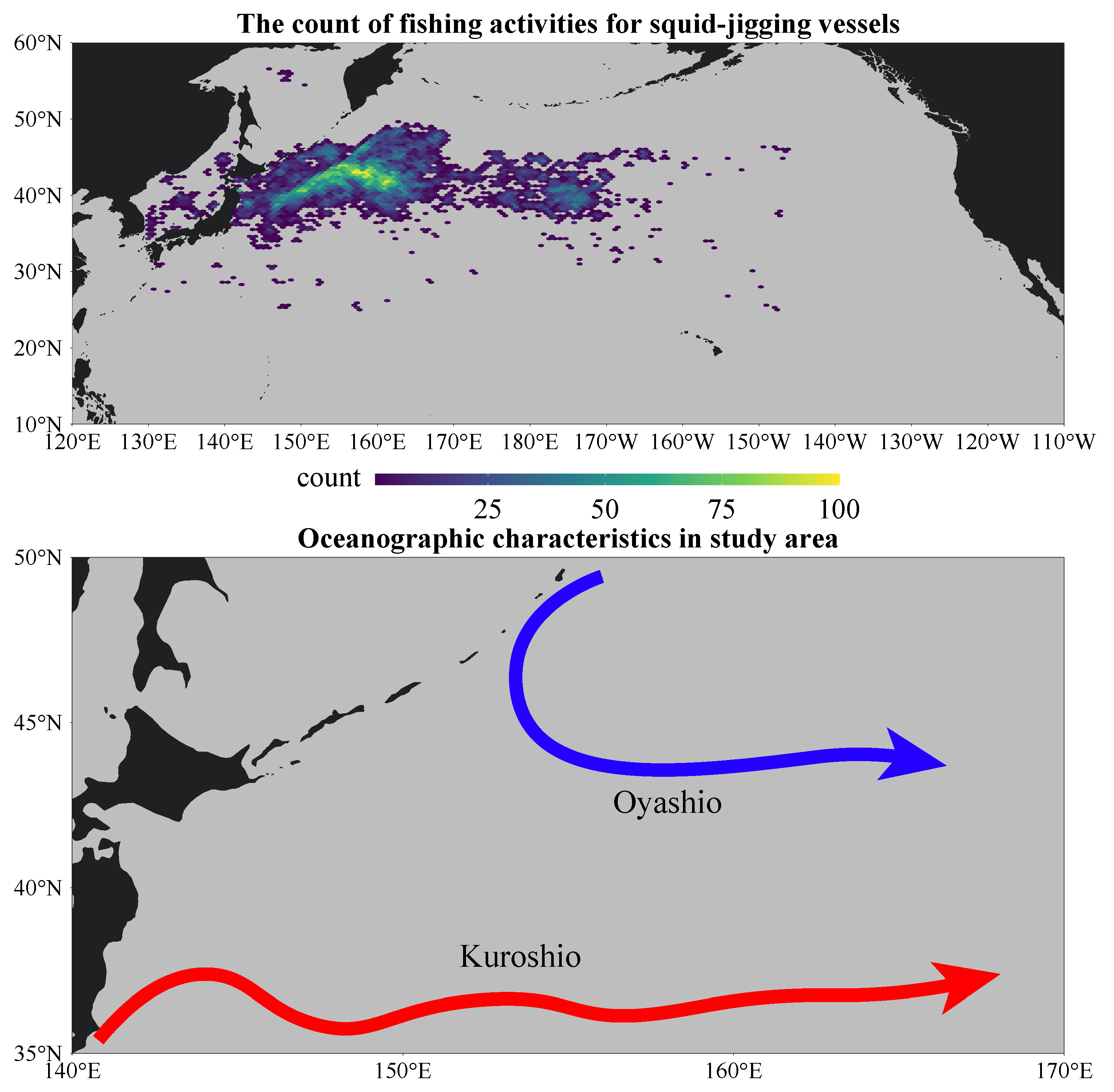
2.1. Study Area

The activity areas of squid-jigging vessels are divided into two parts by approximate 170 E longitude lines (Figure 1). A large number of fishing vessels are concentrated in the western area at 35 N∼50 N, 140 E∼170 E, and only a few fishing vessels occur in the eastern area. Thus, we chose the western area with 35 N∼50 N, 140 E∼170 E as the study area.

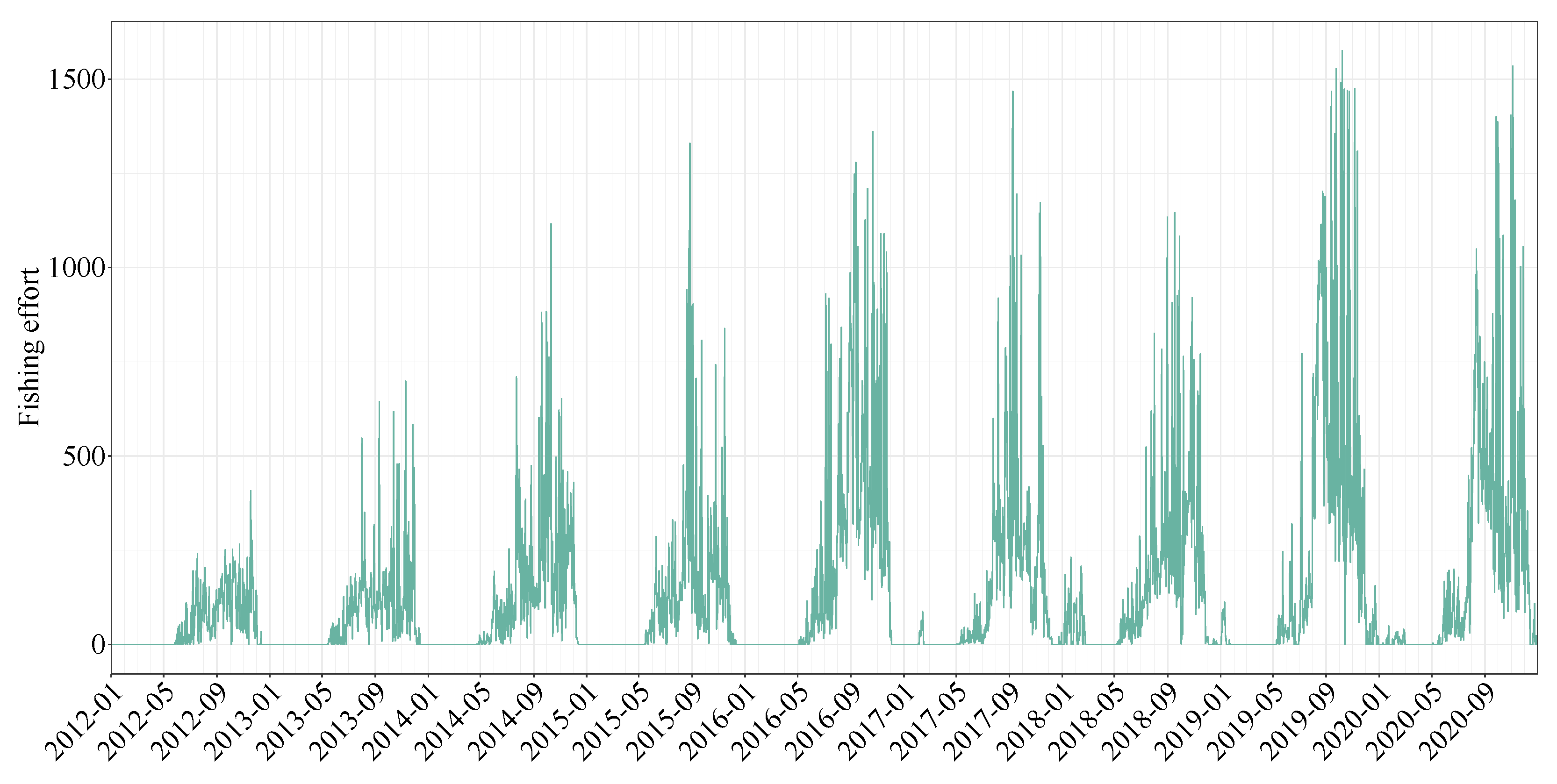
2.2. Fishing Effort Data and Fishery Data

Fishing effort data were downloaded from Global Fishing Watch (GFW, https://globalfishingwatch.org/, accessed on 6 June 2022). The original data include the Maritime Mobile Service Identity (MMSI), type of vessel, date, latitude, longitude, and fishing effort. The spatial and temporal scales of the original data were 0.1 × 0.1 and daily, respectively. The GFW project has developed convolutional neural network (CNN) algorithms to distinguish fishing from non-fishing activities and identify the fishing effort distribution for different fishing gear types at high spatial and temporal resolution [5,21]. Information on squid-jigging vessels in the study area was selected based on the type of vessel. The temporal range of the dataset is from January to December during 2012∼2020. The fishing effort of squid-jigging vessels is at a low level from January to May and in December in each year (Figure 2). Thus, the fishing effort data from June to November were adopted in this study. Previous studies have suggested that the optimal spatial and temporal scales for studying O. bartramii stocks are 0.5 × 0.5 and monthly, respectively [22,23]. Therefore, the spatial and temporal scales of the original fishing effort data were processed into 0.5 × 0.5 and monthly, respectively.
The fishery data were from the commercial fishing data of squid-jigging fishery in the North Pacific Ocean of China. However, we only obtained the data for 2018 due to confidentiality. Commercial fishing data include date (year-month-day), latitude, longitude, and catch (unit: ton). The spatial and temporal scales of the fishery data were also integrated as 0.5 × 0.5 and monthly, respectively.

2.3. Marine Environmental Data

Previous studies have emphasized that the distribution of O. bartramii stocks is influenced by multiple environmental variables [15,24,25,26,27,28,29,30]. Several environmental variables were selected as predictor variables in this study (Table 1). Furthermore, diel vertical swimming is an extremely important habit of O. bartramii, and it mainly inhabits the thermocline at depths of 0∼40 m at night. During the day, O. bartramii lives in deep water, and its maximum depth of swimming is approximately 300 m [31]. Hence, we downloaded environmental data from 0∼300 m depth with an interval of 50 m to explore the impact of environmental factors in deep water on squid-jigging vessels (Table 1).
The environmental data were downloaded from Copernicus Marine Service (https://resources.marine.copernicus.eu/?option=com_csw&task=results, accessed on 6 June 2022). Here, the spatial and temporal scales of the environmental data also were integrated as 0.5 × 0.5 and monthly, respectively, to correspond to fishing effort data.
The formula for calculating eddy kinetic energy (EKE) is as follows [32]:
EKE = u 2 + v 2 2
where u and v are the zonal and meridional components of the geostrophic currents, respectively.

2.4. BRT Model

The BRT models were constructed using two steps in this study. In the first step, BRT models were adopted to obtain the important predictor variables that influence fishing effort and the relative influence of these variables for each month. Here, the top six variables with the highest relative influence were retained as monthly important environmental variables. In the second step, the BRT models were used to assess the relative influence of each important predictor variable for each month.
The BRT model was implemented by using the “gbm.step” function within the “gbm” package in the R language environment. There are three important parameters in the “gbm.step” function: learning rate (lr), tree complexity (tc), and bagging fraction (bf). Elith et al. [33] considered that higher tree complexity and lower learning rate are the preferable combination, and the bagging fraction is proposed to be set at 0.5∼0.75. In view of the above conclusions, (i) the learning rate was preset to 0.01, 0.005 and 0.001, (ii) the tree complexity was preset to 5, 6, 7, and 8, and (iii) the bagging fraction was set to 0.5. Predictive deviance was used to measure which combination of parameters was optimal. After the optimal parameters were selected, we used the 10-fold cross-validation to train the model. The area under the receiver operating characteristic curve (AUC) value was applied to determine the performance of the BRT model and select the optimal model. Manel et al. [34] indicated that if the AUC value of a model is higher than 0.7, then the model performance is good.

2.5. HSI Model

The monthly important environmental variables were used for modelling the HSI models. Here, the data during 2012∼2019 were used as input data for developing the model and the data in 2020 were used as test data for validation. SI values are assessed by dividing the total effort for each environmental class by the maximum effort for a given class in a specific month. The SI values were used to fit the SI curve. The SI curve fitting formula of the environmental variable x is [35]
SI x = exp [ α · ( x β ) 2 ] ,
where α and β are parameters, which are calculated using the least squares estimation. The Python 3.9.2 was applied for fitting SI curves.
The next step was to combine all the SI models into an HSI model. The equations of weighted-AMM and the weighted-GMM in this study, respectively, were
HSI AMM = 1 i = 1 n ω i · i = 1 n SI i · ω i ,
HSI GMM = i = 1 n SI i ω i 1 i = 1 n ω i ,
where SI i is the suitability value of i-th environmental variable; ω i is the weight of the variable based on the relative influence (%) of different important environmental variables according to BRT results; and n is the number of environmental variables included in the HSI model. HSI values range from 0 to 1. The areas with HSI > 0.6, 0.2 < HSI ≤ 0.6, and HSI ≤ 0.2 were defined as suitable, normal, and poor habitats for O. bartramii, respectively [36].
The final step was to validate the HSI model. Each SI model was statistically evaluated. The root mean square error (RMSE), mean absolute error (MAE), and coefficient of determination ( R 2 ) was used to evaluate each SI model. Their formula is as follows:
R M S E = i = 1 n ( y i y ˜ i ) 2 n , M A E = 1 n i = 1 n | y i y ˜ i | , R 2 = 1 i = 1 n ( y i y ˜ i ) 2 i = 1 n ( y i y ¯ ) 2 ,
where y i is the observed value; y ¯ is the average of the observed values; and y ˜ i is the estimated value. The data from June to November in 2020 were used to validate the weighted-AMM models and weighted-GMM models. Furthermore, we counted the fishing effort and frequency of fishing activity under different HSI levels in 2020.

2.6. Suitable Fishing Areas for Squid-Jigging Vessels

The monthly average HSI values in 2012∼2019 were calculated to explore the potential suitable areas related to environmental fishing activities for squid-jigging vessels. Persistence is a measure of the number of months that a location was classified as a suitable habitat throughout the year. The yearly HSI during 2012∼2019 was calculated, and the locations with HSI > 0.6 were classified as 1. To identify areas where favourable environmental conditions for fishing are most stable throughout the year, persistence maps were plotted.

2.7. Evaluating O. bartramii Potential Habitat

To address whether the fishing effort could be an alternative way to understand the habitat suitability index for O. bartramii, the prediction map in 2018 was overlaid with fishery data and compared with fishing effort data, and the statistical index was computed as poor, normal, and suitable habitats regions, respectively.

3. Results

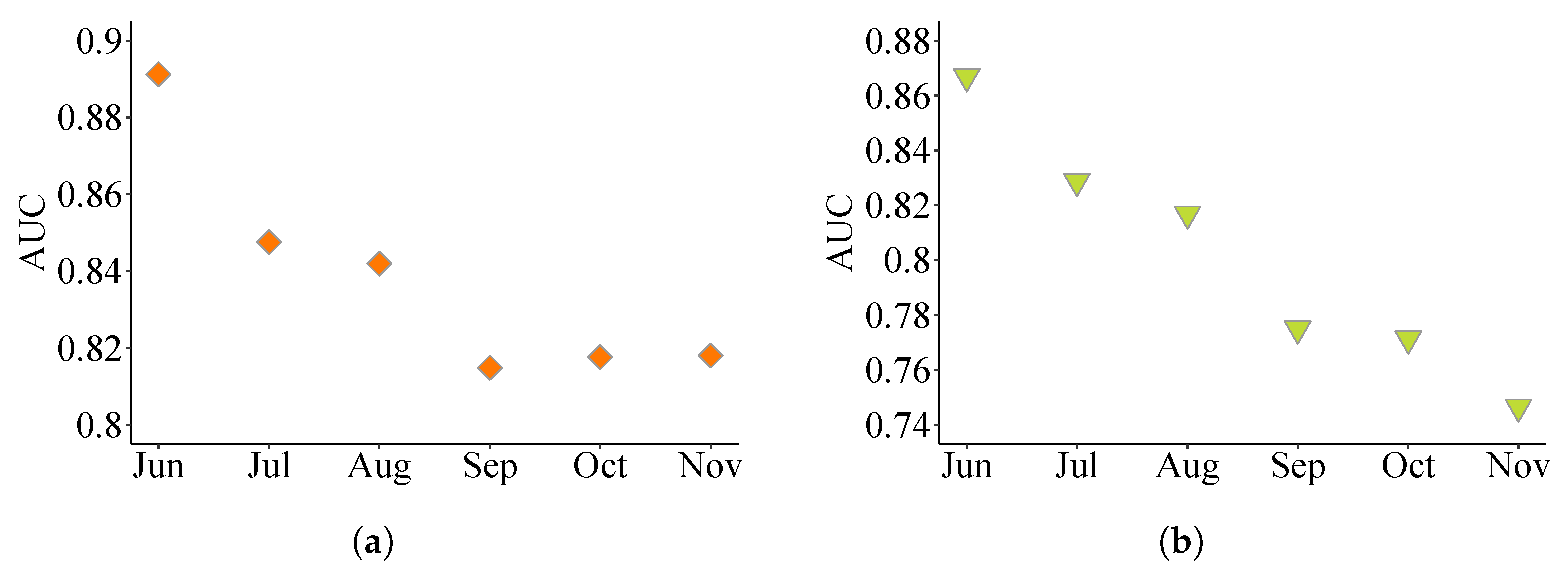
3.1. Parameters and Performance of the BRT Models

The optimal parameters for the first and second BRT models are shown in Table S1 according to predictive deviance (Figures S1a–f and S2a–f). The AUC values of the monthly BRT models in the first modelling were all greater than 0.8 (Figure 3a). The AUC values of the monthly BRT models in the second modelling were all greater than 0.74 (Figure 3b). The performance of monthly optimal BRT models was considered to be good [34].

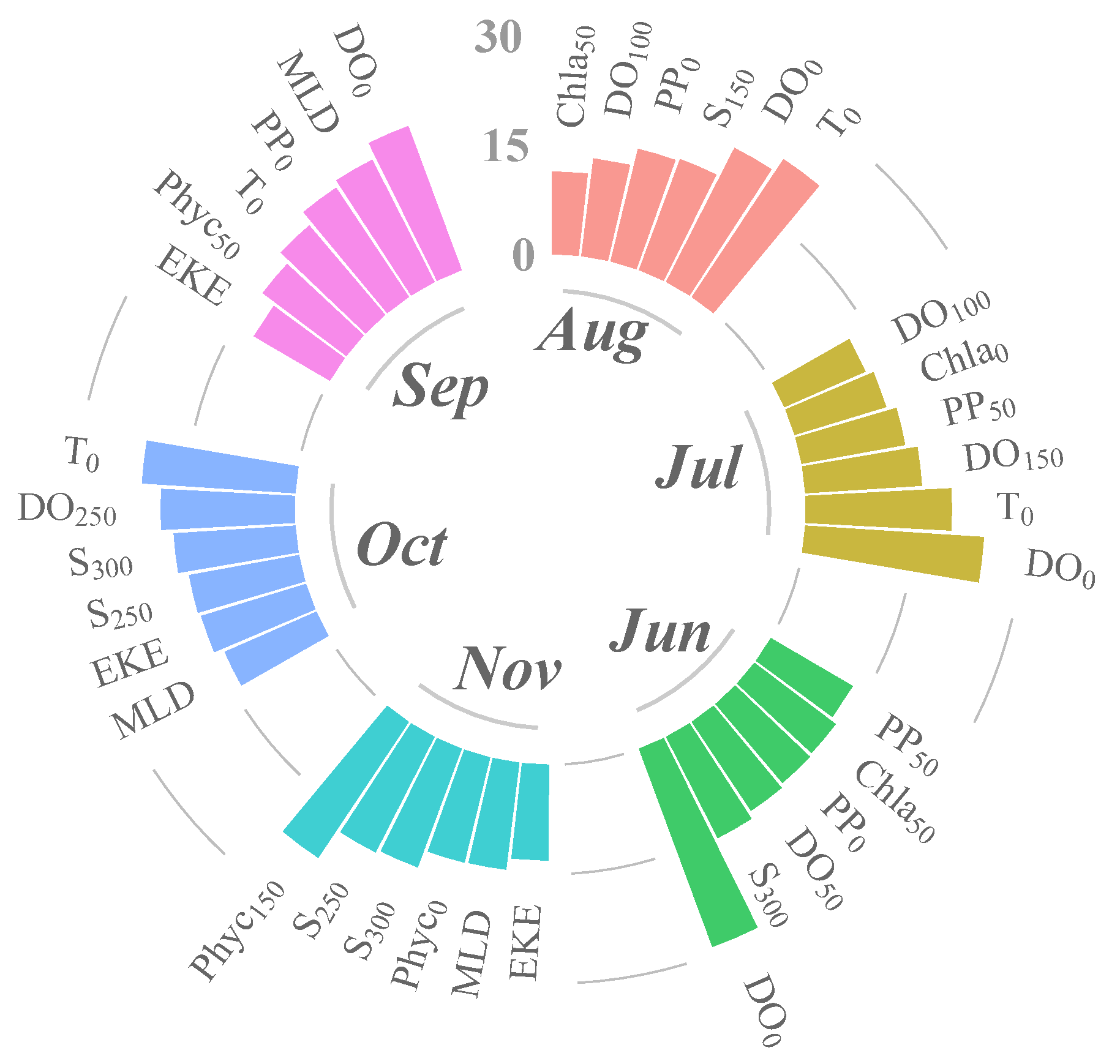
3.2. Relative Influence of Environmental Variables

The relative influences of important environmental variables in each month are shown in Figure 4. The fishing effort of squid-jigging vessels has a significant seasonal preference for oceanographic conditions. DO 0 and T 0 have an important influence on the distribution of fishing activity in most months.

3.3. Analysis of SI Curves

Table S2 showed that the SI model of important environmental variables for each month has excellent statistical performance from June to November. The results showed that the RMSE and MAE of each SI model were low, and the coefficients of determination of the models were high, all above 0.6 (Table S2). Figure S3a–f showed the SI curves for monthly important environmental variables. The favourable ranges of different variables for fishing effort are shown in Table S3.

3.4. Analysis of Different HSI Models

The predicted spatial distribution maps of the HSI values for two different models are shown in Figure 5a,b. Figure 5a,b showed that the spatial distribution of HSI values predicted by weighted-GMM was more significantly variable relative to weighted-AMM. The high fishing effort mainly occurred in the areas with high HSI value, and a few fishing effort occurred in the areas with low HSI value. By comparing the two types of models, the distribution of the areas with high HSI were similar, but they had different performances in low-value regions, especially in July.
The Fishing Effort/Frequency Graphs (Figure 6a,b) showed the fishing activities mainly occurred in the areas with high HSI value. As HSI increased, there was an increasing trend in the frequency of corresponding fishing activities. The results of the weighted-AMM model showed that the fishing effort was mainly distributed in the areas with HSI ≥ 0.5, with a very small percentage in the areas with HSI < 0.5. Conversely, more fishing activities occurred in the areas with HSI ≥ 0.5 based on weighted-GMM. The results of the weighted-AMM model showed that 73.43% of fishing activities and 56,159.1 h of fishing efforts occurred in the suitable habitat areas (Figure 6a). For the weighted-GMM, 52.91% of fishing activities and 46,893.7 h of fishing effort were located in the suitable habitat areas (Figure 6b). The predicted results of the weighted-GMM model were lower than the weighted-AMM model results in the high value range, but higher than the weighted-AMM results in the low value range. This indicated that the results of the weighted-GMM model underestimated the suitable areas for squid-jigging vessel activity. Therefore, according to the previous study [35], the weighted-AMM model was considered to have a better performance for predicting the suitable operation areas.

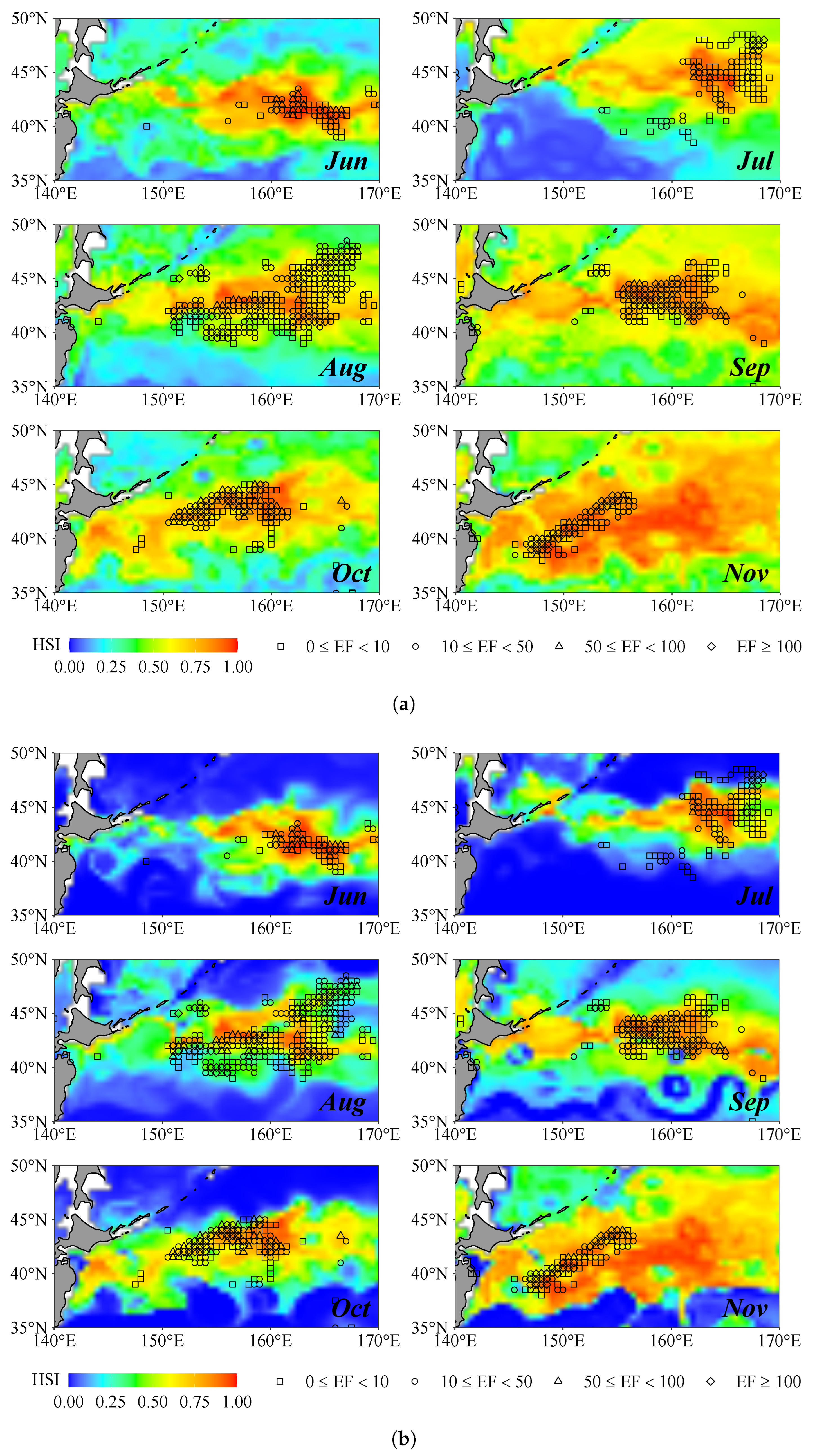
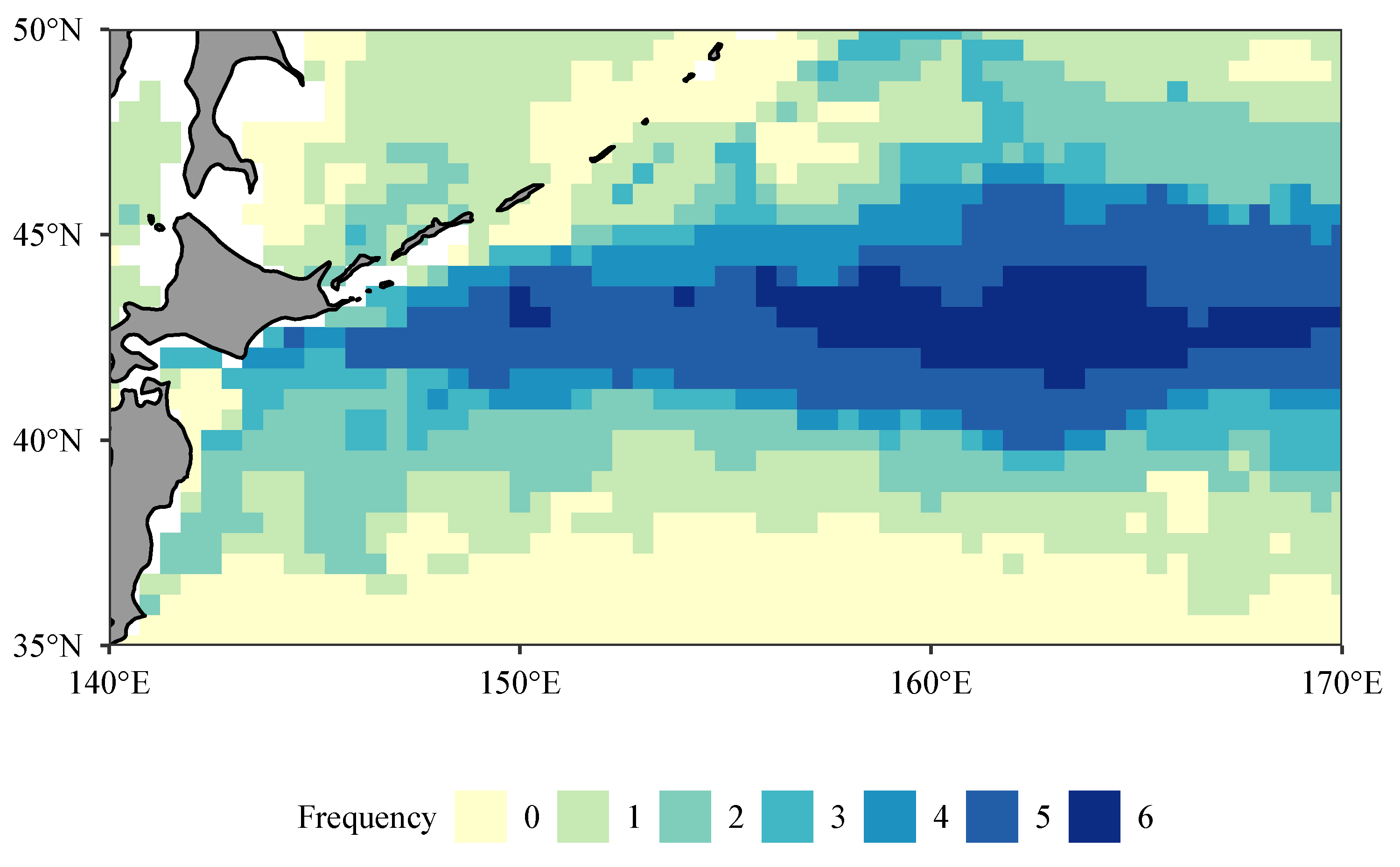
3.5. Spatial Distribution of Hotspots for Fishing

The prediction hotspots for squid-jigging vessels during 2012∼2019 were distributed in the area of 40 N∼45 N in June, August, and September (Figure 7). The hotspots were located in the northeast, which was above approximately 42 N in July. The hotspots gradually extended to the south in October and November. The favourable area covered most of the study area in November.
A suitable fishing region from 2012 to 2019 was observed in the strip area of 40 N∼45 N (Figure 8). The most suitable fishing area (cumulative frequency = 6) for squid-jigging vessels was distributed in the scope of 42 N∼44 N, 155 E∼170 E during 2012∼2019 (Figure 8).

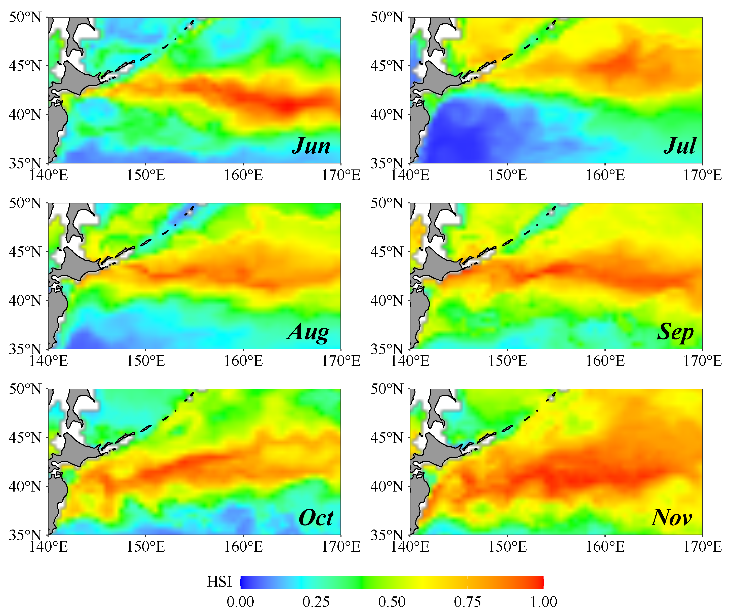
3.6. Revealing Squid Potential Habitat

The weighted-AMM model was adopted to predict the habitat map in 2018, and overlaid with fishery data for O. bartramii. O. bartramii was mainly caught in suitable habitat areas from August to November, but no catches in June and July were observed in suitable habitat areas (Figure S4). A total of 58.1% of fishing activities, with a corresponding catch of 5716.4 t, was located in suitable habitat areas (Table 2). The poor habitats yielded very low catches and fishing efforts.
Compared to fishery data, the fishing efforts in 2018 within different habitat classes (poor, normal, and suitable habitats) were examined. The frequency of fishing activities in poor, normal, and suitable habitats was 5.7%, 37.9% and 56.4%, respectively (Table 2). The fishing efforts rarely occurred in poor habitats (Figure S5). These findings suggest a consistent spatial distribution of fishing activities, catch, and habitat quality, implying the excellent prediction performance of the HSI in our model for fishing habitats.

4. Discussion

Understanding the spatial distribution and hot spots of fishing activity is important for improving sustainable fisheries management and protecting vulnerable fish stocks. In this paper, we explore the spatial ecology of the distribution of squid-jigging vessels fishing in the Northwest Pacific Ocean by constructing the HSI models of fishing distribution from satellite-based AIS data from GFW. The BRT was used to determine which environmental variables were selected and their weights based on their relative importance in the HSI modeling. The results provide an approach to identify areas in the Northwest Pacific Ocean where favorable environmental conditions for squid-jigging vessels fishing are most stable.

4.1. Model Construction

In the previous literature, the input variables in the HSI model were limited to a few surface oceanography factors. We described the distribution of squid-jigging vessels as characterized by a set of environmental and statistical variables in this study. Studies have shown that the vertical structure of variables such as temperature profoundly influences the distribution of squid in the water column [37]. Incorporating a third dimension relating to the vertical positions of marine species into the models could improve their precision and utility [38,39].
Sakurai et al. [40] indicated that different oceanographic conditions may lead to various impacts on squid stocks. Due to the lack of information about the importance of different variables, all environmental variables are considered to have equal importance and are assigned equal weights in establishing the HSI model, which is obviously unrealistic. Xue et al. [41] applied the BRT model to evaluate the relative influence of different environmental variables. To assess the optimum HSI model, the BRT model was adopted to obtain the important variables and their weights. The HSI model had a good capacity to predict habitat suitability for squid-jigging vessels based on the validation results.

4.2. Influence of Oceanographic Conditions

The selected environmental variables and their relative explanatory variable importance fluctuated each month, which suggests that different environmental variables explain the distribution of squid-jigging fishing efforts during different times of the year. Squid-jigging vessels mainly capture O. bartramii in the Northwest Pacific Ocean. The selected environmental factors mainly reflect the physiological and ecological habits of the targeted species.
Sea surface temperature ( T 0 ) is an important factor that influences the distribution of habitats for O. bartramii [16,25,42]. The overall suitable range of T 0 is 14∼19 °C in this study, which is similar to the O. bartramii habitat [29,35,42]. Fishing effort was highly concentrated in waters with low T 0 in July. It seems possible that these results are due to the fact that the O. bartramii stock migrates northwards to the subarctic boundary for feeding during May to July [14], which indirectly leads to the favourable T 0 for fishing efforts being lower in July. Notably, the results of this study found that the influence of T 0 was not significant in certain months, which might be due to the small difference in temperature in the area of fishing vessel activity in certain months.
Figure 4 showed that the fishing effort was evidently influenced by dissolved oxygen at different depths, from June to September. The hatching period for the winter–spring cohort is mainly from January to May, but extends to August, and O. bartramii matures from July to October [43]. It is prudent to speculate that individuals during the early growth period, and the later mating and spawning processes, requires the consumption of a large amount of dissolved oxygen for energy conversion. In addition, squid spawn their eggs on the sea surface for hatching [44], which is possibly an explanation for the more prominent influence of DO 0 .
Yu et al. [29] indicated that variations in the concentration of chlorophyll-a were related to the food availability of squid and mainly influenced the growth of squid populations. Primary production has potential impacts on the distribution and abundance of O. bartramii [45]. According to the diel vertical swimming characteristics of squid, they often feed at night on the surface or in shallow water [14]. Therefore, the above conditions may be responsible for the significant influence of chlorophyll concentration, primary production, and phytoplankton on the fishing effort of squid fishing vessels in shallow water areas during the squid growing season from June to October.
The suitable MLD gradually increases from September to November. Yu et al. [28] indicated that squid tend to congregate if the MLD is in the range of 5∼60 m. The deep mixed layer entrains nutrient-rich water and enhances photosynthesis, which results in good feeding conditions for paralarvae and juveniles [15]. Alabia et al. [42] suggested that the mesoscale variability in the upper ocean inferred from EKE was also influential on squid potential fishing grounds and is presumably linked to the augmented primary productivity from the nutrient enhancement and entrainment of passive plankton. Yu et al. [28] regarded that areas with a high abundance of O. bartramii tend to occur in areas of low EKE. This is similar to our results. Sea water salinity affects the spawning grounds of O. bartramii [24]. The salinity in deeper waters has a significant influence on fishing effort, which might be caused by the southwards migration of squid for spawning from October to November.

4.3. Comparison for HSI Model

For HSI models, the performance of individual SI models significantly affects the reliability of the HSI model [20]. Moreover, different HSI models yield different spatial distributions of HSI values [46]. In this study, two types of HSI models were developed using the weighted-AMM and weighted-GMM, respectively. The results suggest that the weighted-AMM models were more suitable to evaluate the influence of environmental change on the fishing effort of squid-jigging vessels, and could be applied to predict variations in the dynamics of potential habitat for O. bartramii. The AMM was based on the assumption that high HSI values on one variable could compensate for low HSI values on another variable [46]. The SI variables in the GMM model were assumed to be independent but also compensative [19]. Yu et al. [35] emphasized that the results of the HSI model developed using the GMM will be underestimated, and the HSI values may be very low. This is consistent with the results of this study. In fact, the HSI value in some areas was underestimated by weighted-GMM according to Figure 5b, which indicated that the weighted-GMM model was also unable to effectively evaluate the influence of environmental change on the fishing effort of a squid-jigging vessel and inapplicable to predict variations in the dynamics of potential fishing areas for a squid-jigging vessel.

4.4. Analysis of the Suitable Fishing Area for Squid-Jigging Vessels

The monthly persistence maps also help identify areas that are not classified as environmentally suitable for fishing throughout the year, which provides valuable information about which areas may be experiencing less fishing pressure. The optimal area for fishing activities was located in the scope of 42 N∼44 N, 155 E∼170 E (Figure 8). The spatial distribution of monthly suitable fishing areas for squid-jigging vessels has an obvious seasonal variation. Overall, the suitable fishing areas shifted to the north from June to August and shifted to the south from September to November (Figure 7), which is caused by the the north–south migration of O. bartramii stocks for feeding and spawning. The areas where the value was low had strong seasonal variations. Igarashi et al. [47] suggested that the interaction of the warm and nutrient-poor Kuroshio current and the cold and nutrient-rich Oyashio current could provide favorable conditions for the foraging of O. bartramii in unseasonally suitable fishing areas. The higher value reflected the high fishing pressure on ecology. Therefore, greater protection and regulation efforts should be focused on these areas than on the areas where the value is low. Moreover, the areas where the value was low have strong seasonal variations, and seasonal management should be adopted for these areas.

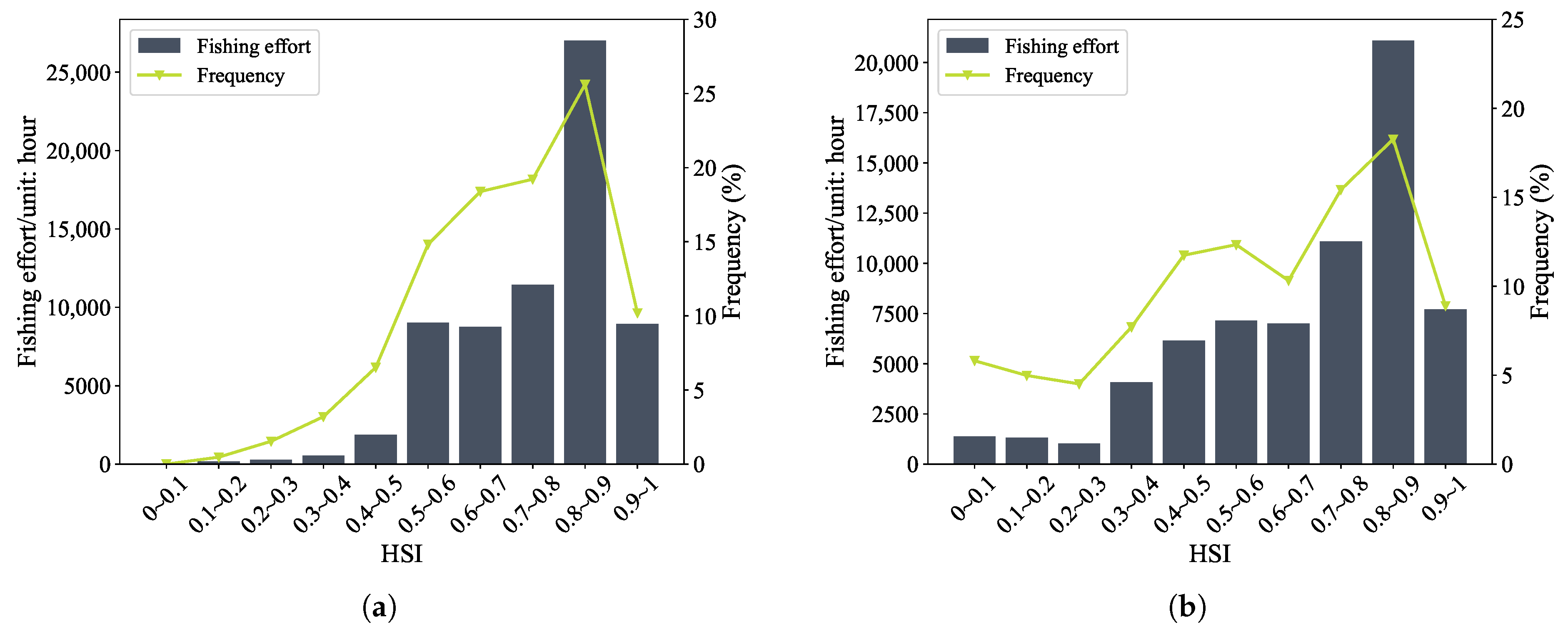
4.5. Fishing Effort in Comparison to Catch

Prior studies have indicated that the CPUE-based HSI model tended to overestimate the ranges of optimal habitats and almost all the study area was classified as optimal habitats, which led to difficulty in analysing monthly changes in squid habitat [20]. Yu and Chen [36] suggested that the CPUE-based HSI model was not applicable to the short-lived O. bartramii stock. In this study, fishing effort was defined as the time of fishing activities for squid-jigging vessels at a location, which reflects the level of satisfaction of fishermen with the catch in the area [48]. If the catch in an area is low, fishing vessels do not remain there for an extended period of time [20]. Therefore, if the fishing vessel spends a longer time fishing, this reflects the fact that a large number of fishing vessels were gathered in an area, which might indicate that environmental conditions in the area were favourable for squid and consequently drove massive squid aggregations and attracted fishing vessels [49]. According to the above considerations, it is reasonable and appropriate to use the HSI model based on fishing efforts for detecting suitable habitats [46].
The spatial distribution of Chinese vessel activity is different from the global fishing effort, especially in June and July (Figures S4 and S5). The spatial distribution of fishery data represents most of the fishing activity for the Chinese squid-jigging vessels because the captains operate based on experience and they may exchange experience with each other. Chinese squid-jigging vessels contributed to the fishing efforts located in the high seas in June and July (Figure S4). This also suggests differences in the distribution of fishing activity between countries or regions. The fishery data from one country or region are restricted by spatial and temporal distribution and fishing experience, which probably biases the results of the study. Alabia et al. [42] suggested that the assessment of a potential fishing habitat for squid may be biased due to limitations in the spatial coverage of fisheries data. This reveals that fishing effort data derived from AIS data could be used as an alternative in fisheries research.

4.6. Perspectives for Fisheries Management

Perspectives for management policy: In the Northwest Pacific Ocean, the regional fisheries management organisations have adopted the boarding inspection method to inspect whether the fishing vessel is conducting operations in accordance with regulations. Additionally, there were no fishing quotas or establishment of protection zones in the areas, aince boarding inspection has high costs and supervision coverage is limited. Thus, it is not possible to fully and effectively monitor the operation of fishing vessels. Under the limited fisheries regulatory force, identifying the hotspot areas of fishing activities for squid-jigging vessel and targeted dispatch of high seas enforcement fleets to focus on monitoring fishing hotspots and ecologically vulnerable areas can significantly provide efficiency in the regulation of fishing vessels. Furthermore, in the areas of high fishing pressure, the establishment of protection zones, closure of certain fishing areas, and implementation of conservation measures for marine species can increase the efficiency in protecting marine organisms and revive the ecological balance of the area.
This study considered the lack of representativeness of fisheries data, which possibly leads to incomplete researches for fisheries resources and management. Therefore, identifying the hotspot areas and its dynamic variation, and dispatching fishery observers to the hotspot areas, were significantly important for improving the representativeness of fisheries data. Meanwhile, the spatial accuracy of fisheries data should be focused on checking. Moreover, some satellite-based data can also complement traditional fisheries data, such as AIS and VMS (vessel-monitoring systems).

5. Conclusions

In this study, the fishing efforts derived from AIS data were used to analyse the suitability of fishing areas for squid-jigging vessels. The BRT model could be effectively used to obtain the weights for the HSI model; the weighted-AMM has a better predicting performance and it was well-suited for predicting suitable fishing areas. The predicted suitable areas and fishery data exhibited excellent spatial consistency. The HSI model, based on fishing effort, could be used to explore potential habitats for O. bartramii. The results also showed a new approach to support fishery management for addressing IUU issues.

Supplementary Materials

The following supporting information can be downloaded at: https://www.mdpi.com/article/10.3390/fishes8100530/s1, Figure S1: Predictive deviance under different learning rates and complexities for each month when the BRT model was first developed; Figure S2: Predictive deviance under different learning rates and complexities for each month when the BRT model was second developed; Figure S3: The SI curves of important variables for each month; Figure S4: Monthly distribution for O. bartramii in the Northwest Pacific Ocean in 2018, overlaid on the habitat class map which was predicted by using weighted-AMM based on environmental data from 2018; Figure S5: Monthly distribution of fishing effort for squid-jigging vessel in the Northwest Pacific Ocean in 2018, overlaid on the habitat class map which was predicted by using weighted-AMM based on environmental data from 2018; Table S1: Optimal parameters for the first and second construction of the BRT model; Table S2: Statistical parameters for each SI model; Table S3: The favorable range of different variables for fishing effort.

Author Contributions

Conceptualisation, Y.F. and S.Y. (Shenglong Yang); methodology, S.Y. (Shenglong Yang), Y.F. and M.H.; software, S.Y. (Shenglong Yang); validation, S.Y. (Shenglong Yang), W.F. and S.Y. (Sanling Yuan); formal analysis, W.F. and S.Y. (Sanling Yuan); investigation, Y.F. and S.Y. (Shenglong Yang); data curation, F.T.; writing—original draft preparation, Y.F.; writing—review and editing, S.Y. (Shenglong Yang); visualisation, Y.F., X.W., Z.Y. and J.Z.; supervision, W.F. and S.Y. (Sanling Yuan); project administration, W.F. and S.Y. (Shenglong Yang). All authors have read and agreed to the published version of the manuscript.

Funding

This research was funded by the Laoshan Laboratory (LSKJ202201804), the Special Funds of Basic Research of Central Public Welfare Institute (2019T09), the Natural Science Foundation of Shanghai (23ZR1445100), and the National Natural Science Foundation of China (12071293).

Data Availability Statement

Publicly available datasets of vessel numbers were analysed in this study. These data can be found here: https://globalfishingwatch.org, accessed on 6 June 2022. And environmental data can be found here: https://data.marine.copernicus.eu/products?option=com_csw&task=results, accessed on 6 June 2022.

Acknowledgments

The authors of this research would like to thank all the researchers who contributed to the research process during our study. We are thankful, also, for the data that were provided by Global Fishing Watch and Copernicus Marine Service.

Conflicts of Interest

The authors declare no conflict of interest.

References

  1. Cimino, M.A.; Anderson, M.; Schramek, T.; Merrifield, S.; Terrill, E.J. Towards a Fishing Pressure Prediction System for a Western Pacific EEZ. Sci. Rep. 2019, 5, 461. [Google Scholar] [CrossRef] [PubMed]
  2. Natale, F.; Gibin, M.; Alessandrini, A.; Vespe, M.; Paulrud, A. Mapping Fishing Effort through AIS Data. PLoS ONE 2015, 10, e0130746. [Google Scholar] [CrossRef] [PubMed]
  3. Damien, L.G.; Cyril, R.; Françoise, G.; David, B. Defining high-resolution dredge fishing grounds with Automatic Identification System (AIS) data. Aquat. Living Resour. 2017, 30, 39. [Google Scholar] [CrossRef]
  4. Ferrà, C.; Tassetti, A.N.; Grati, F.; Pellini, G.; Polidori, P.; Scarcella, G.; Fabi, G. Mapping change in bottom trawling activity in the Mediterranean Sea through AIS data. Mar. Policy 2018, 94, 275–281. [Google Scholar] [CrossRef]
  5. Kroodsma, D.A.; Mayorga, J.; Hochberg, T.; Miller, N.A.; Boerder, K.; Ferretti, F.; Wilson, A.; Bergman, B.; White, T.D.; Block, B.A.; et al. Tracking the global footprint of fisheries. Science 2018, 359, 904–908. [Google Scholar] [CrossRef]
  6. Le Tixerant, M.; Le Guyader, D.; Gourmelon, F.; Queffelec, B. How can Automatic Identification System (AIS) data be used for maritime spatial planning? Ocean. Coast. Manag. 2018, 166, 18–30. [Google Scholar] [CrossRef]
  7. Russo, E.; Monti, M.A.; Mangano, M.C.; Raffaetà, A.; Sarà, G.; Silvestri, C.; Pranovi, F. Temporal and spatial patterns of trawl fishing activities in the Adriatic Sea (Central Mediterranean Sea, GSA17). Ocean. Coast. Manag. 2020, 192, 105231. [Google Scholar] [CrossRef]
  8. White, T.D.; Ferretti, F.; Kroodsma, D.A.; Hazen, E.L.; Carlisle, A.B.; Scales, K.L.; Bograd, S.J.; Block, B.A. Predicted hotspots of overlap between highly migratory fishes and industrial fishing fleets in the northeast Pacific. Sci. Adv. 2019, 5, eaau3761. [Google Scholar] [CrossRef]
  9. Selig, E.; Nakayama, S.; Wabnitz, C.; Österblom, H.; Spijkers, J.; Miller, N.; Bebbington, J.; Sparks, J. Revealing global risks of labor abuse and illegal, unreported, and unregulated fishing. Nat. Commun. 2022, 13, 1612. [Google Scholar] [CrossRef]
  10. Yang, S.; Zhang, H.; Fan, W.; Shi, H.; Fei, Y.; Yuan, S. Behaviour Impact Analysis of Tuna Purse Seiners in the Western and Central Pacific Based on the BRT and GAM Models. Front. Mar. Sci. 2022, 9, 881036. [Google Scholar] [CrossRef]
  11. Fei, Y.; Yang, S.; Fan, W.; Shi, H.; Zhang, H.; Yuan, S. Relationship between the Spatial and Temporal Distribution of Squid-Jigging Vessels Operations and Marine Environment in the North Pacific Ocean. J. Mar. Sci. Eng. 2022, 10, 550. [Google Scholar] [CrossRef]
  12. Arkhipkin, A.I.; Rodhouse, P.G.K.; Pierce, G.J.; Sauer, W.; Sakai, M.; Allcock, L.; Arguelles, J.; Bower, J.R.; Castillo, G.; Ceriola, L.; et al. World Squid Fisheries. Rev. Fish. Sci. Aquac. 2015, 23, 92–252. [Google Scholar] [CrossRef]
  13. Dong, E.; Shi, S.; He, J.; Tang, F. On state of squid jigging fishery and professional upgrading transformation of squid fishing vessels in the North Pacific—Take China Aquatic Products Zhoushan Marine Fisheries Co., LTD as an example. Fish. Inf. Strategy 2020, 35, 208–215. [Google Scholar] [CrossRef]
  14. Watanabe, H.; Kubodera, T.; Ichii, T.; Kawahara, S. Feeding habits of neon flying squid Ommastrephes bartramii in the transitional region of the central North Pacific. Mar. Ecol. Prog. Ser. 2004, 266, 173–184. [Google Scholar] [CrossRef]
  15. Nishikawa, H.; Toyoda, T.; Masuda, S.; Ishikawa, Y.; Sasaki, Y.; Igarashi, H.; Sakai, M.; Seito, M.; Awaji, T. Wind-induced stock variation of the neon flying squid (Ommastrephes bartramii) winter-spring cohort in the subtropical North Pacific Ocean. Fish. Oceanogr. 2015, 24, 229–241. [Google Scholar] [CrossRef]
  16. Anderson, C.I.; Rodhouse, P.G. Life cycles, oceanography and variability: Ommastrephid squid in variable oceanographic environments. Fish. Res. 2001, 54, 133–143. [Google Scholar] [CrossRef]
  17. Brander, K. Impacts of climate change on fisheries. J. Mar. Syst. 2010, 79, 389–402. [Google Scholar] [CrossRef]
  18. Brown, S.K.; Buja, K.R.; Jury, S.H.; Monaco, M.E.; Banner, A. Habitat Suitability Index Models for Eight Fish and Invertebrate Species in Casco and Sheepscot Bays, Maine. N. Am. J. Fish. Manag. 2000, 20, 408–435. [Google Scholar] [CrossRef]
  19. Chang, Y.J.; Sun, C.L.; Chen, Y.; Yeh, S.Z.; DiNardo, G.; Su, N.J. Modelling the impacts of environmental variation on the habitat suitability of swordfish, Xiphias gladius, in the equatorial Atlantic Ocean. ICES J. Mar. Sci. 2013, 70, 1000–1012. [Google Scholar] [CrossRef]
  20. Tian, S.; Chen, X.; Chen, Y.; Xu, L.; Dai, X. Evaluating habitat suitability indices derived from CPUE and fishing effort data for Ommatrephes bratramii in the northwestern Pacific Ocean. Fish. Res. 2009, 95, 181–188. [Google Scholar] [CrossRef]
  21. de Souza, E.N.; Boerder, K.; Matwin, S.; Worm, B. Improving Fishing Pattern Detection from Satellite AIS Using Data Mining and Machine Learning. PLoS ONE 2016, 11, e0158248. [Google Scholar] [CrossRef]
  22. Gong, C.; Chen, X.; Gao, F.; Tian, S. Effect of spatial and temporal scales on habitat suitability modeling: A case study of Ommastrephes bartramii in the Northwest Pacific Ocean. J. Ocean Univ. China 2014, 13, 1043–1053. [Google Scholar] [CrossRef]
  23. Feng, Y.; Cui, L.; Chen, X.; Chen, L.J.; Yang, Q. Impacts of changing spatial scales on CPUE-factor relationships of Ommastrephes bartramii in the northwest Pacific. Fish. Oceanogr. 2019, 28, 143–158. [Google Scholar] [CrossRef]
  24. Ichii, T.; Mahapatra, K.; Sakai, M.; Inagake, D.; Okada, Y. Differing body size between the autumn and the winter-spring cohorts of neon flying squid (Ommastrephes bartramii) related to the oceanographic regime in the North Pacific: A hypothesis. Fish. Oceanogr. 2004, 13, 295–309. [Google Scholar] [CrossRef]
  25. Nishikawa, H.; Igarashi, H.; Ishikawa, Y.; Sakai, M.; Kato, Y.; Ebina, M.; Usui, N.; Kamachi, M.; Awaji, T. Impact of paralarvae and juveniles feeding environment on the neon flying squid (Ommastrephes bartramii) winter–spring cohort stock. Fish. Oceanogr. 2014, 23, 289–303. [Google Scholar] [CrossRef]
  26. Wang, J.; Yu, W.; Chen, X.; Lin, L.; Chen, Y. Detection of potential fishing zones for neon flying squid based on remote-sensing data in the Northwest Pacific Ocean using an artificial neural network. Int. J. Remote Sens. 2015, 36, 3317–3330. [Google Scholar] [CrossRef]
  27. Wang, J.; Cheng, Y.; Lu, H.; Chen, X.; Lin, L.; Zhang, J. Water Temperature at Different Depths Affects the Distribution of Neon Flying Squid (Ommastrephes bartramii) in the Northwest Pacific Ocean. Front. Mar. Sci. 2022, 8, 741620. [Google Scholar] [CrossRef]
  28. Yu, W.; Chen, X.; Yi, Q.; Chen, Y. Spatio-temporal distributions and habitat hotspots of the winter-spring cohort of neon flying squid Ommastrephes Bartramii in relation to oceanographic conditions in the Northwest Pacific Ocean. Fish. Res. 2016, 175, 103–115. [Google Scholar] [CrossRef]
  29. Yu, W.; Chen, X.; Yi, Q.; Chen, Y. Influence of oceanic climate variability on stock level of western winter-spring cohort of Ommastrephes bartramii in the Northwest Pacific Ocean. Int. J. Remote Sens. 2016, 37, 3974–3994. [Google Scholar] [CrossRef]
  30. Chen, P.; Chen, X.; Yu, W.; Lin, D. Interannual Abundance Fluctuations of Two Oceanic Squids in the Pacific Ocean Can Be Evaluated through Their Habitat Temperature Variabilities. Front. Mar. Sci. 2021, 8, 770224. [Google Scholar] [CrossRef]
  31. Murata, M.; Nakamura, Y.N. Seasonal migration and diel vertical migration of the neon flying squid, Ommastrephes bartramii in the North Pacific. In Proceedings of the International Symposium on Large Pelagic Squids; Okutani, T., Ed.; Japan Marine Fishery Resources Research Center: Yokohama, Japan, 1998; pp. 13–30. [Google Scholar]
  32. Scharffenberg, M.G.; Stammer, D. Seasonal variations of the large-scale geostrophic flow field and eddy kinetic energy inferred from the TOPEX/Poseidon and Jason-1 tandem mission data. J. Geophys. Res. Oceans 2010, 115. [Google Scholar] [CrossRef]
  33. Elith, J.; Leathwick, J.R.; Hastie, T. A working guide to boosted regression trees. J. Anim. Ecol. 2008, 77, 802–813. [Google Scholar] [CrossRef] [PubMed]
  34. Manel, S.; Williams, H.C.; Ormerod, S. Evaluating presence-absence models in ecology: The need to account for prevalence. J. Appl. Ecol. 2001, 38, 921–931. [Google Scholar] [CrossRef]
  35. Yu, W.; Chen, X.; Zhang, Y.; Yi, Q. Habitat suitability modelling revealing environmental-driven abundance variability and geographical distribution shift of winter–spring cohort of neon flying squid Ommastrephes bartramii in the northwest Pacific Ocean. ICES J. Mar. Sci. 2019, 76, 1722–1735. [Google Scholar] [CrossRef]
  36. Yu, W.; Chen, X. Habitat suitability response to sea-level height changes: Implications for Ommastrephid squid conservation and management. Aquac. Fish. 2021, 6, 309–320. [Google Scholar] [CrossRef]
  37. Alabia, I.D.; Saitoh, S.I.; Igarashi, H.; Ishikawa, Y.; Usui, N.; Kamachi, M.; Awaji, T.; Seito, M. Ensemble squid habitat model using three-dimensional ocean data. ICES J. Mar. Sci. 2016, 73, 1863–1874. [Google Scholar] [CrossRef]
  38. Brodie, S.; Jacox, M.G.; Bograd, S.J.; Welch, H.; Dewar, H.; Scales, K.L.; Maxwell, S.M.; Briscoe, D.M.; Edwards, C.A.; Crowder, L.B.; et al. Integrating Dynamic Subsurface Habitat Metrics Into Species Distribution Models. Front. Mar. Sci. 2018, 5, 219. [Google Scholar] [CrossRef]
  39. Melo-Merino, S.M.; Reyes-Bonilla, H.; Lira-Noriega, A. Ecological niche models and species distribution models in marine environments: A literature review and spatial analysis of evidence. Ecol. Model. 2020, 415, 108837. [Google Scholar] [CrossRef]
  40. Sakurai, Y.; Kiyofuji, H.; Saitoh, S.I.; Yamamoto, J.; Goto, T.; Mori, K.; Kinoshita, T. Stock fluctuations of the Japanese common squid, Todarodes pacificus, related to recent climate changes. Fish. Sci. 2002, 68, 226–229. [Google Scholar] [CrossRef]
  41. Xue, Y.; Guan, L.; Tanaka, K.; Li, Z.; Chen, Y.; Ren, Y. Evaluating effects of rescaling and weighting data on habitat suitability modeling. Fish. Res. 2017, 188, 84–94. [Google Scholar] [CrossRef]
  42. Alabia, I.D.; Saitoh, S.I.; Mugo, R.; Igarashi, H.; Ishikawa, Y.; Usui, N.; Kamachi, M.; Awaji, T.; Seito, M. Seasonal potential fishing ground prediction of neon flying squid (Ommastrephes bartramii) in the western and central North Pacific. Fish. Oceanogr. 2015, 24, 190–203. [Google Scholar] [CrossRef]
  43. Bower, J.R.; Ichii, T. The red flying squid (Ommastrephes bartramii): A review of recent research and the fishery in Japan. Fish. Res. 2005, 76, 39–55. [Google Scholar] [CrossRef]
  44. Young, R.E.; Hirota, J. Description of Ommastrephes bartramii (Cephalopoda: Ommastrephidae) Paralarvae with Evidence for Spawning in Hawaiian Waters. Pac. Sci. 1990, 44, 71–80. [Google Scholar]
  45. Ichii, T.; Mahapatra, K.; Sakai, M.; Okada, Y. Life history of the neon flying squid: Effect of the oceanographic regime in the North Pacific Ocean. Mar. Ecol. Prog. Ser. 2009, 378, 1–11. [Google Scholar] [CrossRef]
  46. Yu, W.; Yi, Q.; Chen, X.; Chen, Y. Modelling the effects of climate variability on habitat suitability of jumbo flying squid, Dosidicus gigas, in the Southeast Pacific Ocean off Peru. ICES J. Mar. Sci. 2015, 73, 239–249. [Google Scholar] [CrossRef]
  47. Igarashi, H.; Saitoh, S.I.; Ishikawa, Y.; Kamachi, M.; Usui, N.; Sakai, M.; Imamura, Y. Identifying potential habitat distribution of the neon flying squid (Ommastrephes bartramii) off the eastern coast of Japan in winter. Fish. Oceanogr. 2018, 27, 16–27. [Google Scholar] [CrossRef]
  48. Bordalo-Machado, P. Fishing Effort Analysis and Its Potential to Evaluate Stock Size. Rev. Fish. Sci. 2006, 14, 369–393. [Google Scholar] [CrossRef]
  49. Chen, X.; Tian, S.; Chen, Y.; Liu, B. A modeling approach to identify optimal habitat and suitable fishing grounds for neon flying squid (Ommastrephes bartramii) in the Northwest Pacific Ocean. Fish. Bull. Natl. Ocean. Atmos. Adm. 2010, 108, 1–14. [Google Scholar]
Figure 1. Spatial distribution of traditional fishing ground for the winter–spring cohort of neon flying squid in the North Pacific Ocean.
Fishes 08 00530 g001
Figure 2. Temporal distribution of fishing effort for squid-jigging vessel from 2012 to 2020.
Fishes 08 00530 g002
Figure 3. (a) AUC values of the monthly optimal BRT model in first modelling. (b) AUC values of the monthly optimal BRT model in second modelling.
Fishes 08 00530 g003
Figure 4. The relative influence of important environmental variables (%) for each month.
Fishes 08 00530 g004
Figure 5. Monthly distribution of fishing effort for squid-jigging vessel in the Northwest Pacific Ocean in 2020, overlaid on the HSI maps which were predicted by using weighted-AMM (a) and weighted-GMM (b), respectively, based on environmental data from 2020.
Fishes 08 00530 g005
Figure 6. (a) Fishing effort and frequency of fishing operations in 2020 based on AMM. (b) Fishing effort and frequency of fishing operations in 2020 based on GMM.
Fishes 08 00530 g006
Figure 7. Monthly distribution of hotspots for squid-jigging vessels during 2012∼2019.
Fishes 08 00530 g007
Figure 8. The frequency of locations with HSI > 0.6 from June to November during 2012∼2019.
Fishes 08 00530 g008
Table 1. Marine environmental variables.
VariablesAbbreviationUnits
Water temperature (dm) T d C
Chlorophyll-a (dm) Chla d mg · m 3
Salinity (dm) S d 10 3 (dimensionless)
Primary production (dm) PP d mg · m 3 · day 1
Dissolved oxygen (dm) DO d mmol · m 3
Phytoplankton concentration (dm) Phyc d mg · m 3 · day 1
Sea surface high SSH m
Mixed layer depth MLD m
Eddy kinetic energy EKE m 2 · s 2
d = 0 ,   50 ,   100 ,   150 ,   200 ,   250 ,   300 ; Unit: m.
Table 2. Yield and frequency of catch and fishing effort within different habitat classes.
Habitat ClassEffortCatch
Yield (h)Frequency (%)Yield (t)Frequency (%)
Poor866.65.7194.910.8
Normal11,116.537.9604.531.1
Suitable34,355.556.45716.458.1
Disclaimer/Publisher’s Note: The statements, opinions and data contained in all publications are solely those of the individual author(s) and contributor(s) and not of MDPI and/or the editor(s). MDPI and/or the editor(s) disclaim responsibility for any injury to people or property resulting from any ideas, methods, instructions or products referred to in the content.

