Genetic Diversity and Population Structure of Shoshone Sculpin Cottus greenei in the Hagerman Valley of South-Central Idaho

Abstract

The Shoshone sculpin Cottus greenei is a micro-endemic species and an extreme habitat specialist, geographically restricted to the spring outlets that flow from the Snake River Plain Aquifer into the Snake River within the Hagerman Valley of south central Idaho. Although previous studies documented the range of the species and its relative abundance, no studies have assessed genetic diversity and structure. We sampled 20 populations from throughout the species range and genotyped 1311 with a panel of 12 microsatellite loci. Results indicate very high levels of genetic differentiation among most populations (average pairwise F_ST = 0.24), indicating limited gene flow. Preservation of the genetic diversity of this species will require the protection and preservation of multiple isolated populations.

1. Introduction

Groundwater-fed springs often provide unique environments that support endemic species of plants and animals. Some of the largest springs in the United States are found along the Snake River Canyon in south central Idaho [1]. The water from these springs originates in the mountains of the Lost River Basin where it flows in a southerly direction before disappearing underground into the state’s largest aquifer. After traveling ~160 km south, through porous basalt lava flows, this water returns to the surface along the canyon walls of the Thousand Springs formation before entering the Snake River. This region of springs is constricted to a ~64 km area within the Hagerman Valley, Idaho. The springs have been heavily developed for irrigation and aquaculture [2]. The remaining unaltered springs are characterized by clear, well oxygenated water, and uniform year-round temperatures (14 °C–16 °C) that support a variety of specialist plant and animal species, including three endemic freshwater snail species that are federally protected under the United States Endangered Species Act (ESA) [3].

The springs additionally support the endemic Shoshone sculpin Cottus greenei. Shoshone sculpin are a member of the Cottidae family and were originally described by Gilbert and Culver in 1898 [4]. Recent mitochondrial DNA analyses indicate that Shoshone sculpin are the most divergent member within the C. beldingii complex, under the Subgenus Uranidea [5]. Populations of Shoshone sculpin have only been found in 25 locations, all of which are immediately adjacent to springs or spring influenced outlet streams [4]. Shoshone sculpin are a short-lived species (~3 years), reaching sexual maturity after their first year, with a total length of only 7–10 cm [6]. The species was petitioned for listing under the ESA in 1979, prompting a status review (53 FR 52746). Several studies were performed in response to that status review, documenting the species distribution and relative abundance [4,7], and a decision of “not warranted” was issued. The species is currently ranked as imperiled globally [8] and is considered imperiled by the Idaho Department of Fish and Game and a “species of greatest information need” [9].

Despite its conservation status, no information is currently available about the species genetic diversity and structure. Previous research on a variety of sculpin species indicate that they often exhibit significant genetic differentiation among populations, even at very small distances. Studies on bullhead C. gobio, found high differentiation among populations separated by 35 km [10]. Research on mottled sculpin C. bairdi showed evidence of strong isolation by distance among locations spanning only 5.6 km [11]. The reasons for this observed high structuring is variable, attributed to both low dispersal range [12] and natural or anthropogenic isolation [10].

Over the last 100 years, the middle Snake River, from C.J. Strike Reservoir to American Falls Dam has been transformed by dams, water withdrawals and diversions, and water pollution [13], likely making it inhospitable to the movement of sculpin between the spring habitats. As such, one could expect to see high genetic differentiation among spring populations due to reduced connectivity and genetic drift. However, population surveys indicate that some of these populations are quite large [6]. Even with a fast generation time, fragmentation of these populations may be too recent to detect significant genetic structuring even in the face of little to no connectivity.

Here, we provide the first estimates of genetic diversity, structure, and effective population size of this Idaho endemic, using range-wide sampling and microsatellite DNA analyses.

2. Methods

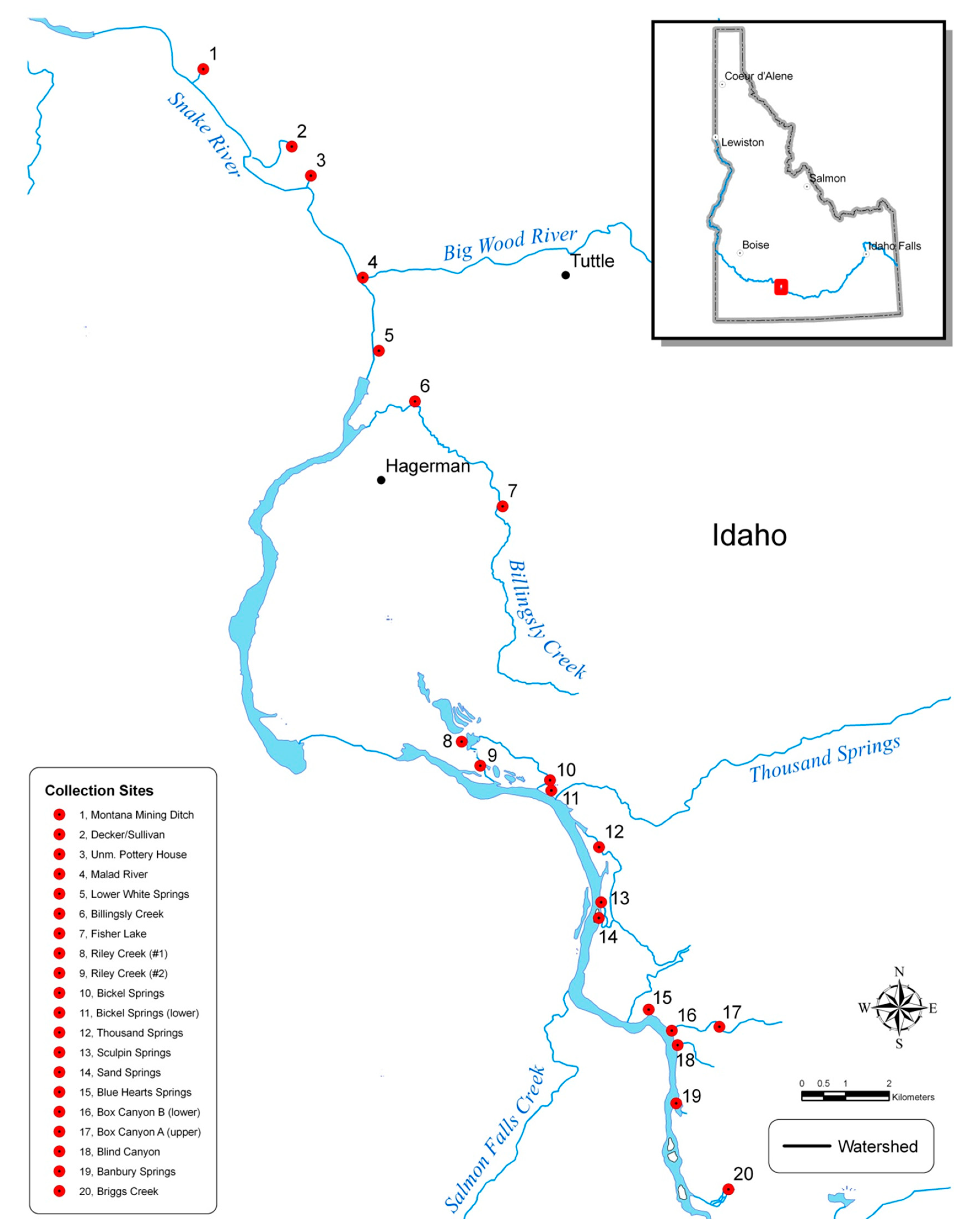
2.1. Population Sampling

Shoshone sculpin were sampled from 20 sites over a three-year period (2008–2010) using either electroshocking techniques or minnow traps (

Table 1. Population, collection site #, year sampled, sample size (N), expected and observed heterozygosity (H_E and H_O, respectively), number of alleles per locus (N_A), and effective population size (N_E) estimates from LDNE (with 95% lower and upper confidence intervals) of 20 Shoshone sculpin collection sites sampled in 2008, 2009, and 2010. Upper confidence intervals with an estimate of infinity are marked with an ∞.

Population	Collection Site #	Year	N	HE	HO	NA	NE	NE (95% L)	NE (95% U)
Montana Mining Ditch	1	2009	35	0.38	0.37	3.1	−131.8	68.2	∞
Decker/Sullivan	2	2009	70	0.37	0.38	3.4	−6256.8	95	∞
Unm. Pottery House	3	2009	53	0.35	0.34	3.1	441.1	61.3	∞
Malad River	4	2008	49	0.50	0.49	4.9	−1972.7	128.4	∞
Lower White Springs	5	2009	80	0.48	0.49	4.9	937.5	126.5	∞
Billingsley Creek	6	2008	50	0.33	0.32	2.7	114.5	34.1	∞
Fisher Lake	7	2010	50 *	0.36	0.36	4.9	149.8	37	∞
Riley Creek (upper)	8	2009	57	0.39	0.38	4.1	687.9	100.1	∞
Riley Creek (lower)	9	2009	54	0.62	0.61	6.7	271.2	82.1	∞
Bickel Springs (upper)	10	2008	50	0.36	0.35	3.3	131.9	32.6	∞
Bickel Springs (lower)	11	2009	50	0.61	0.59	6.4	19,674.3	224.5	∞
Thousand Springs	12	2008	50	0.62	0.59	7.2	132.4	69.2	605.3
Sculpin Springs	13	2008	50	0.62	0.62	6.7	175	77.2	∞
Sand Springs	14	2008	50	0.62	0.59	7.0	−1169.3	226.1	∞
Blue Hearts Springs	15	2008	23	0.55	0.59	4.4	270.4	43.5	∞
Box Canyon (lower)	16	2008	50	0.57	0.56	6.1	131.1	50.8	∞
Box Canyon (upper)	17	2008	49	0.46	0.43	4.3	150.8	56.4	∞
Blind Canyon	18	2009	55	0.56	0.55	5.8	1485.7	106	∞
Banbury Springs	19	2008	56	0.33	0.32	4.3	186.2	48.3	∞
Briggs Creek	20	2009	65	0.22	0.22	2.4	−230.3	83.2	∞

* The total number of samples that were genotyped from Fisher Lake was 315. A random sample of 50 individuals were used for diversity and N_E comparisons.

and Figure 1). We followed American Fisheries Society guidelines for fish collection and sampling [14]. A non-lethal fin tissue sample was taken from each fish and stored in 100% non-denatured ethanol. Technicians were provided photographs and diagnostic phenotypic characteristics to differentiate mottled sculpin C. bairdii from Shoshone sculpin at sample sites. Ten fish from each site were kept following fin tissue sampling to serve as voucher specimens and were sent to the Orma J. Smith Museum of Natural History in Caldwell, Idaho (Donald W. Zaroban, Curator of Fishes) for archiving.

2.2. DNA Extraction and Microsatellite DNA Optimization and Screening

We could find no published results indicating that microsatellite DNA loci had ever been developed specifically for Shoshone sculpin, nor any evidence that Shoshone sculpin had ever been screened with microsatellite DNA loci developed in other sculpin species. To identify useful loci for this study, we tested 40 microsatellite DNA loci demonstrated to amplify in other Cottus species–primarily the mottled sculpin (C. bairdii) [15] and the European bullhead (C. gobio) [16,17]. We tested these markers on a small sample of Shoshone sculpin (N = 24) and mottled sculpin (N = 6) from Banbury Springs, ID. Mottled sculpin were included to act as an amplification control and to determine whether any loci might be useful in differentiating species and testing for hybridization.

Of the 40 loci tested, 21 were dropped from consideration due to failure to amplify, no allelic variation, or difficulties in scoring (stutter or adenylation issues). Of the remaining 19 loci, we further excluded 7 that exhibited lower genetic diversity so that we could optimize the remaining 12 loci into two multiplex PCR panels (Panel A and B). The 12 loci were Cba42, Cott100, Cott105, Cott113, Cott130, Cott207, CottES10 (Panel A) and Cgo310, Cgo1114, Cgo33, Cott118, and LCE89 (Panel B). Most of the loci used in this study either do not amplify in mottled sculpin or exhibit allele sizes that are diagnostic between the two species, allowing us to check phenotypic identifications. Primer sequences for these loci are reported in

Table 2. The 12 microsatellite loci that were used in this study optimized to allow evaluation in two PCR multiplex reactions/panels (A and B). Locus name, primer names, dye, primer sequences, allelic range in b.p. observed across all populations in this study, number of alleles observed (A^O) across all populations in this study, whether the locus appears to be diagnostic between C. greenei and C. bardii (D^M), and reference for each locus.

Panel	Locus	Primer Names	Dye	Primer Sequences	Range b.p.	AO	DM	Reference
A	Cba42	Cba42F	VIC	AAATGGTCGTCTGCTCCCTG	110–129	9	N	[15]
		Cba42R		AGGCAGTGTGGGCATGAAAG
A	Cott100	Cott100F	NED	CTCATCGTGGTTTGATCGGTG	178–194	7	Y	[17]
		Cott100-PIG R		CCGAGCGTGAGTCAGGCGTG
A	Cott105	Cott105F	NED	TCCTACAGGGTGCGATCGTG	305–320	7	N	[17]
		Cott105R		TGCAGGAGTCAGGACTCTGC
A	Cott113	Cott113F	6FAM	AGCGCCAGAATGCAGCATCC	139–166	10	Y	[17]
		Cott113R		AGTGTGGCGAGCCCAAGATC
A	Cott130	Cott130F	PET	TCTGGATCCCTCGGACCAGG	152–177	10	Y	[17]
		Cott130-PIG R		TGAGCTCCATCGTGGGTTCG
A	Cott207	Cott207F	PET	AGTCCTTGTCGGGAGCCTCG	299–347	18	N	[17]
		Cott207R		ATTGGGCGTTGCTCACCAGC
A	CottES10	CottES10F	VIC	CAGGCGGCGACACGGTG	175–197	10	N	[17]
		CottES10R		TTATGAGGAGTCTGCCAATGCAG
B	Cgo310	Cgo310F	6FAM	AGAACCAGTGTTTGACTCTGC	181–209	13	Y	[16]
		Cgo310R		CACTGTCATGTAGCGGCTC
B	Cgo1114	Cgo1114F	6FAM	GTGACTGAGCCTTGAGATTC	109–147	15	N	[16]
		Cgo1114R		GAACCAACGGAAATGAAAC
B	Cgo33	Cgo33F	PET	CAAAAGACAGACCTGTTGAC	153–193	13	N	[16]
		Cgo33-PIG R		TTAACAGTGAAGGATGTGAG
B	Cott118	Cott118F	PET	ACTGGTCTCCAGGCGGTGTC	383–395	6	Y	[17]
		Cott118R		GACGCCGTCATGCTCAGGTC
B	LCE89	LCE89F	6FAM	AGAGCACACACCCTTCCGGTC	260–328	12	N	[17]
		LCE89R		GAACCTGCACAGGGCTACAGC

. The PCR amplification mix consisted of 2 μL of PCR multiplex kit (QIAGEN), 0.2 μL of primer mix (0.03–0.10 μM of each fluorescently labeled forward and reverse primer pooled) (Table 2), 1 μL of template DNA (20–40 ng) and water to bring the final volume to 5 μL. We used the following PCR cycling parameters: 15 min of denaturation at 95 °C, followed by 30 cycles of 30 s at 94 °C, 90 s at 63 °C (panel A) or 57 °C (panel B) and 60 s extension at 72 °C, followed by a final extension of 30 min at 60 °C. Resulting amplification products for each panel were sized by capillary electrophoresis on an automated ABI 3100 using the molecular standard GeneScan-500 LIZ and GeneMapper 3.5.1 software (Applied Biosystems, Waltham, MA, USA).

2.3. Statistical Analyses

Data generated for each population was tested for Hardy–Weinberg equilibrium (HWE) and linkage disequilibrium with GENEPOP on the Web [18]. An alpha value of 0.05 was chosen for statistical significance, but was adjusted for multiple tests using Bonferroni’s correction [19]. Genetic diversity was measured by the number of alleles per locus (N_A), observed heterozygosity (H_O), and expected heterozygosity (H_E) using the Microsatellite Toolkit for Microsoft Excel™ [20].

GENEPOP on the Web was used to perform exact tests to assess the significance of allelic differentiation between pairs of populations and to estimate pairwise population differentiation (F_ST) [21]. To examine genetic relationships among populations, genetic distances [22] between all populations were estimated in GENDIST in PHYLIP (version 3.5c, Older versions of PHYLIP (washington.edu) accessed on 14 January 2023) [23]. A neighbor-joining dendrogram was generated from these genetic chord distances with the program FITCH in PHYLIP. Bootstrap replicates of 1000 iterations were attained with SEQBOOT and a consensus tree was formed with CONSENSE in PHYLIP. The dendrogram generated in PHYLIP was plotted as a radial tree using TREEVIEW (version 1.6.6, [24].

To test whether genetic differentiation between collection sites was associated with geographic distance, a Mantel’s test [25] was performed from the comparison of population pairwise FST/(1-FST) values against population pairwise straight line geographical distances (Ln) using the program ISOLDE in GENEPOP.

Contemporary effective population size, N_E, was estimated with the linkage disequilibrium (LD) method of Waples [26] using the software program LDNE [27]. Alleles with a frequency < 0.02 were excluded to decrease bias [26] and confidence intervals were estimated with the jackknife method. Sample sizes for most collection sites averaged ~50. However, over 340 samples were collected from Fisher Lake and 315 were genotyped. To test the influence of sample size on N_E estimates [28], we ran LDNE with sample sizes from Fisher Lake of 50, 100, 150, 200, 250, and 300.

Regarding estimates of contemporary N_E; these can be made from a single year sample (e.g., linkage-disequilibrium method), but are based on several assumptions including that samples are drawn from one breeding generation [26]. In situations where samples are drawn from a population with overlapping generations but cohorts can be identified, it is still possible to provide an estimate of N_B (the effective number of breeders that produced the sample) [26]. An attempt was made to age Shoshone sculpin from several sites using otoliths. However, clear annual growth increment patterns were not present in the samples examined (Liz Mamer, IDFG, personal communication). In this study, estimates of effective size were still calculated using LD procedures from samples of adults that were likely of mixed ages. However, the effects of age structure have not been rigorously evaluated for any single-sample N_E estimator, and it was recognized that the resulting values would likely be estimating something intermediate between N_B and N_E [29] and might be imprecise and difficult to interpret.

To assess whether populations showed evidence of undergoing a recent bottleneck or expansion event, we tested for heterozygote excess or deficiency, respectively, using the software program BOTTLENECK 1.2.02 [30,31]. The significance of the test was assessed using Sign, Wilcoxon, and L-shape tests under the stepwise mutation (SMM) and two-phase mutation models (TPM) suggested for microsatellite evolution. Populations that have experienced a recent bottleneck will exhibit a significant (p < 0.05) excess of heterozygosity in these tests [30].

3. Results

3.1. Tests for Hardy-Weinberg Equilibrium and Linkage Disequilibrium

A total of 1,311 Shoshone sculpin samples were included in analyses. Of 240 tests (20 collection sites × 12 loci) for deviations from HWE, 10 were significant at α = 0.05, but this was not higher than expected by chance (240 × 0.05 = 12 expected from type I error of 0.05) and no collection sites or loci consistently deviated from HWE. No HWE tests were significant following Bonferroni correction (0.05/240 = 0.0002). Of the 1320 tests for LD (12 loci × 12 = 144 − 12 = 132/2 = 66 × 20 collection sites = 1320), 82 were significant at α = 0.05, which was slightly higher than expected by chance (1320 × 0.05 = 66 expected from type I error of 0.05). However, no more than four tests clustered around a particular locus pair, and only two tests were significant following Bonferroni correction (0.05/1320 = 0.00004), indicating that none of these loci were closely linked.

We observed seven samples with genotypes indicative of mottled sculpin. All were from Briggs Creek. These samples were removed from further analyses. No samples exhibited genotypes with both mottled sculpin and Shoshone sculpin alleles, indicative of hybrids.

Across the 20 populations examined, the total number of alleles per locus observed ranged from seven alleles at Cott105 and Cott118 to 25 alleles at Cott207. Populations exhibited large variation in genetic diversity among sites (Table 1). Nine sites exhibited heterozygosity estimates lower than 40% (average 33.9%; range 21.9% to 39.2%). Allelic variation in these populations averaged 3.5 (range 2.4 to 4.9). The remaining 11 sites exhibited heterozygosity estimates greater than 45% (average 56.3%; range 45.7% to 62.1%). Allelic variation in these populations averaged 5.8 (range 4.3 to 7.2).

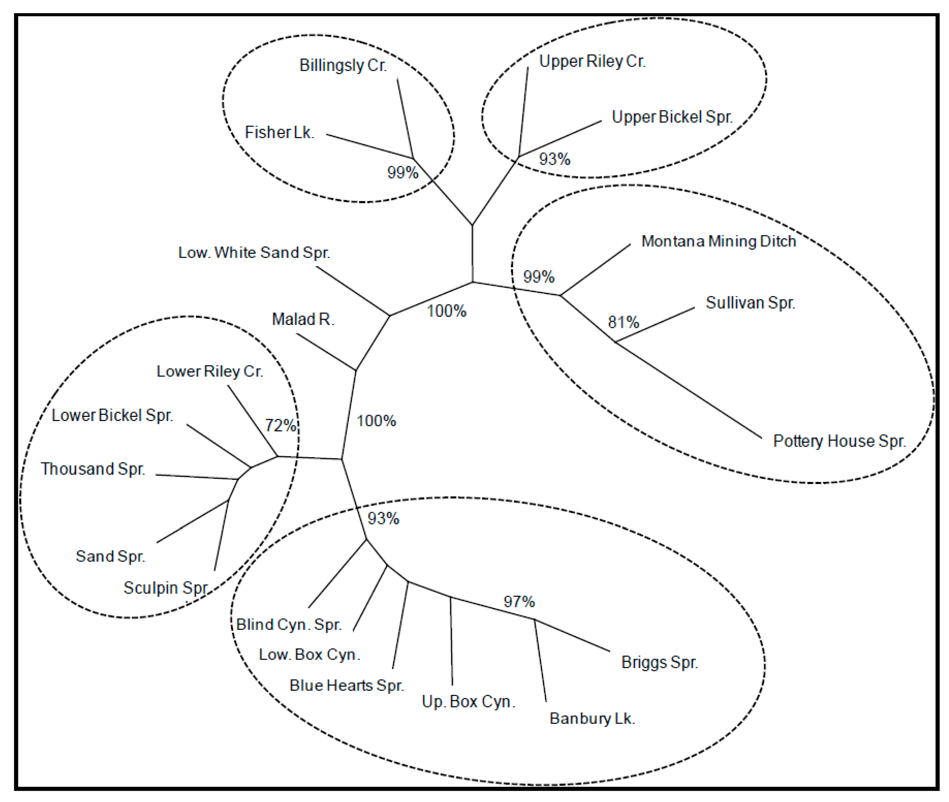
3.2. Genetic Differentiation and Structure

The level of genetic differentiation, as measured by F_ST estimates, ranged from <0.001 (eight pairwise comparisons) to 0.62 for Pottery House Springs and Briggs Springs (

Table 3. Pairwise F_ST among the 20 populations. Numbers in superscript next to Population name corresponds to locations on map (Figure 1).

Population	Montana 1 Mining Ditch	Decker 2/ Sullivan	Unm. 3 Pottery House	Malad 4 River	Lower 5 White Springs	Billingsley 6 Creek	Fisher 7 Lake	Riley 8 Creek (upper)	Riley 9 Creek (lower)	Bickel 10 Springs (upper)	Bickel 11 Springs (lower)	Thousand 12 Springs	Sculpin 13 Springs	Sand 14 Springs	Blue 15 Hearts Springs	Box 16 Canyon (lower)	Box 17 Canyon (upper)	Blind 18 Canyon	Banbury 19 Springs
Decker/Sullivan 2	0.01
Unm. Pottery House 3	0.06	0.04
Malad River 4	0.21	0.24	0.23
Lower White Springs 5	0.20	0.23	0.22	0.02
Billingsley Creek 6	0.26	0.27	0.27	0.17	0.15
Fisher Lake 7	0.25	0.27	0.27	0.20	0.17	0.01
Riley Creek (upper) 8	0.12	0.14	0.19	0.26	0.22	0.21	0.21
Riley Creek (lower) 9	0.26	0.30	0.29	0.11	0.12	0.24	0.28	0.28
Bickel Springs (upper) 10	0.23	0.25	0.25	0.23	0.19	0.12	0.14	0.12	0.26
Bickel Springs (lower) 11	0.29	0.32	0.31	0.11	0.13	0.26	0.29	0.30	<0.00	0.28
Thousand Springs 12	0.30	0.34	0.33	0.12	0.14	0.27	0.31	0.32	<0.00	0.30	<0.00
Sculpin Springs 13	0.30	0.33	0.33	0.12	0.15	0.28	0.32	0.31	<0.00	0.30	<0.00	<0.00
Sand Springs 14	0.30	0.33	0.33	0.13	0.15	0.29	0.32	0.32	0.01	0.30	<0.00	<0.00	<0.00
Blue Hearts Springs 15	0.35	0.38	0.40	0.18	0.21	0.39	0.41	0.37	0.09	0.37	0.10	0.09	0.06	0.07
Box Canyon (lower) 16	0.32	0.36	0.37	0.16	0.18	0.36	0.40	0.35	0.07	0.35	0.08	0.08	0.05	0.06	<0.00
Box Canyon (upper) 17	0.37	0.42	0.43	0.26	0.27	0.44	0.46	0.41	0.17	0.42	0.18	0.17	0.16	0.17	0.13	0.09
Blind Canyon 18	0.32	0.35	0.36	0.16	0.19	0.35	0.39	0.35	0.07	0.34	0.09	0.08	0.06	0.07	<0.00	<0.00	0.10
Banbury Springs 19	0.51	0.52	0.53	0.30	0.33	0.51	0.51	0.51	0.20	0.51	0.20	0.18	0.17	0.18	0.15	0.14	0.25	0.13
BriggsCreek 20	0.60	0.59	0.62	0.38	0.39	0.60	0.55	0.59	0.29	0.59	0.31	0.29	0.26	0.27	0.24	0.20	0.36	0.19	0.15

). The distance between Pottery House Springs (third farthest downstream location) and Briggs Spring (farthest upstream location) is ~45 km. The largest distance between sites that exhibited an F_ST < 0.001 was ~3.5 km (Riley Creek and Sand Springs). All but two population pairwise exact tests (lower Riley Creek versus Sand Springs and Sculpin Springs) were highly significant and the average pairwise F_ST across all sites was 0.24, indicating significant genetic differentiation among most sites.

The neighbor-joining dendrogram indicated that genetic population structuring was generally correlated to geography (Figure 2). Populations (#1–3, 6 and 7) from creeks and springs entering the Snake River north of Hagerman, Idaho, clustered together with 100% bootstrap support. Populations (#9 and #11–20) from creeks and springs entering the Snake River south of Hagerman (upstream) clustered together with 100% bootstrap support. The exceptions to this pattern were lower White Sand Springs (#5) and the Malad River (#4), which did not cluster with any populations, and two isolated populations on upper Riley Creek (#9) and upper Bickel Springs (#11), which are located south of Hagerman, but cluster with downstream collection sites.

Finer-scale structure among geographically proximate sites was also observed (Figure 2). Starting downstream (site #1) and moving upstream; samples from Montana Mining Ditch, Sullivan Springs, and Pottery House Springs (#1, 2, and 3) clustered together with 99% bootstrap support. Samples from Billingsley Creek (#6) and Fisher Lake (#7), both in the Billingsley Creek drainage, clustered together with 99% bootstrap support. Samples from lower Riley Creek (#9), lower Bickel Springs (#11), Thousand Springs (#12), Sculpin Springs (#13), and Sand Springs (#14) clustered together with 72% bootstrap support. Finally, samples from Blue Hearts Spring (#15), lower Box Canyon (#16), upper Box Canyon (#17), Blind Canyon (#18), Banbury Springs (#19), and Briggs Creek (#20) all clustered together with 93% bootstrap support.

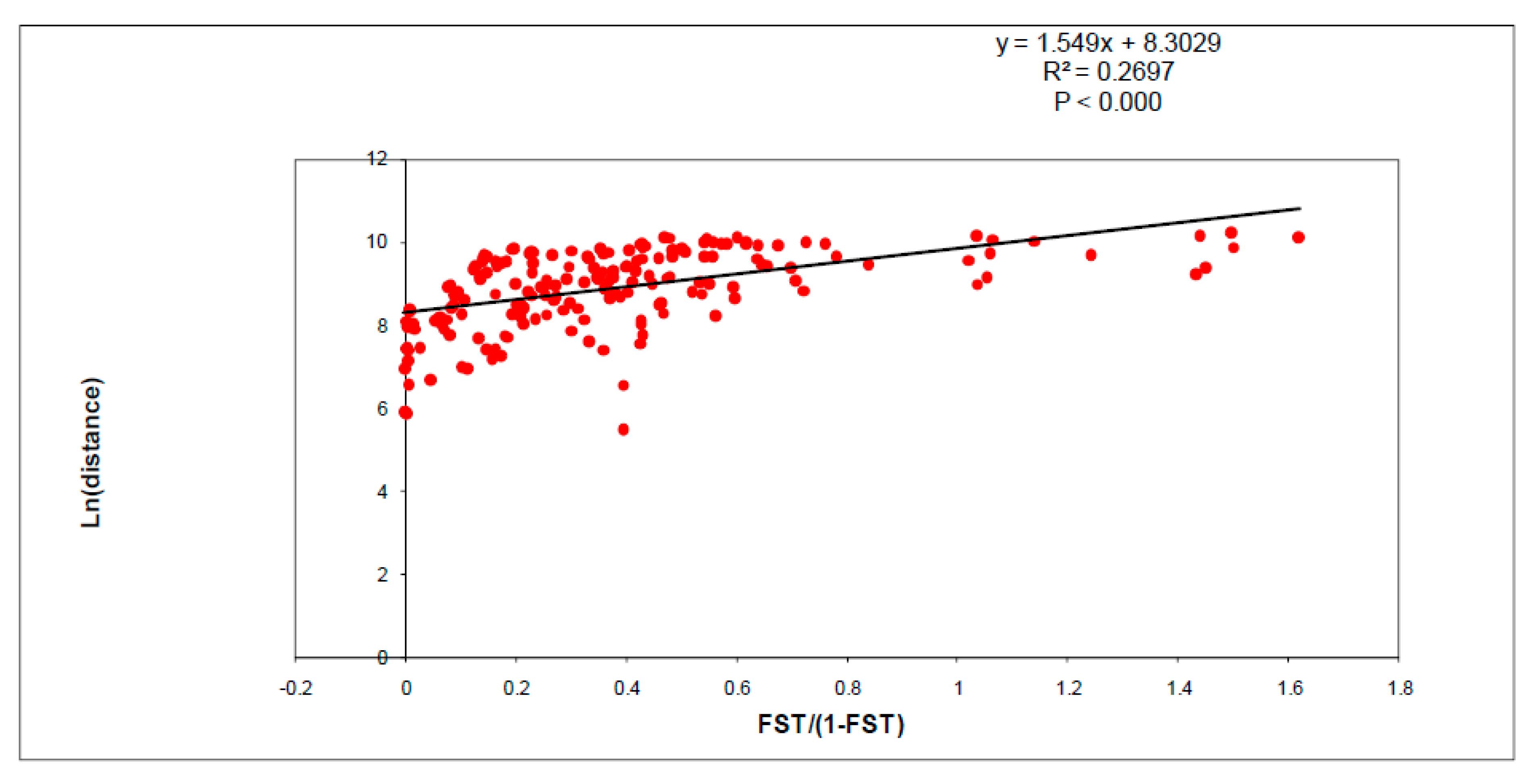
3.3. Isolation by Distance, Effective Population Size, and Bottlenecks

A significant pattern of isolation by distance was observed from the comparison of genetic and geographic distance for the 20 study populations (Figure 3; R² = 0.27, p-value < 0.0001).

Effective population size estimates using LDNE were highly variable among sites (Table 1). Of the positive point estimates observed, Billingsley Creek (#6) had the lowest N_E estimate (114.5) and lower Bickel Springs had the highest (19674.3). Corresponding confidence intervals for all but one population included infinity. Five sites yielded negative point estimates. Negative point estimates can be interpreted as either the population is large enough that drift is insignificant or that the sample size is too low to estimate N_E [26].

The test of adjusting sample sizes (50–300) for the Fisher Lake population also yielded large variations in N_E estimates (

Table 4. Effective population size (N_E) estimates from LDNE (with 95% C.I) of varying sample sizes (N = 50, 100, 150, 200, 250, 300) for the Fisher Lake population. Upper confidence intervals with an estimate of infinity are marked with an ∞.

N	NE	NE(95%L)	NE(95%U)
50	149.8	37.0	∞
100	329.9	91.9	∞
150	4119.4	207.5	∞
200	−1473.6	487.8	∞
250	1729.6	277.8	∞
300	2156.2	401.1	∞

). The smallest estimate of N_E was observed with a sample size of 50 (149.8) and the largest was observed with a sample size of 150 (4119.4). The sample size of 200 yielded a negative point estimate and sample sizes of 250 and 300 yielded estimates of 1729.6 and 2156.2, respectively. Corresponding confidence intervals for all six samples sizes included infinity.

No populations showed evidence of a recent bottleneck under any of the three tests for both mutational models (

Table 5. Tests for past bottlenecks in population size using two tests (Sign and Wilcoxon) under two models of microsatellite mutation: two-phase model (TPM) and stepwise mutation model (SMM). Populations that have experienced a recent bottleneck will show a higher than expected heterozygosity and tests for excess heterozygosity are significant when p-values are <0.05. For the Sign test, the number of loci with heterozygosity deficiency (D) is shown out of the total loci that were examined (12).

Population	Collection Site #	Sign Test TPM	Sign Test SMM	Wilcoxon Test (Deficiency) TPM	Wilcoxon Test (Excess) TPM	Wilcoxon Test (Deficiency) SMM	Wilcoxon Test (Excess) SMM
Montana Mining Ditch	1	0.57	0.31	0.52	0.52	0.31	0.72
Decker/Sullivan	2	0.30	0.12	0.31	0.72	0.12	0.90
Unm. Pottery House	3	0.32	0.13	0.28	0.74	0.08	0.94
Malad River	4	0.13	0.04 D8/12	0.21	0.82	0.01	0.99
Lower White Springs	5	0.08	0.00 D10/12	0.06	0.95	0.00	1.00
Billingsley Creek	6	0.47	0.24	0.72	0.31	0.28	0.75
Fisher Lake	7	0.02 D9/12	0.00 D11/12	0.02	0.99	0.00	1.00
Riley Creek (upper)	8	0.21	0.07	0.22	0.81	0.01	0.99
Riley Creek (lower)	9	0.07	0.00 D10/12	0.10	0.91	0.00	1.00
Bickel Springs (upper)	10	0.54	0.25	0.31	0.72	0.10	0.92
Bickel Springs (lower)	11	0.36	0.00 D10/12	0.34	0.69	0.00	1.00
Thousand Springs	12	0.16	0.00 D112/12	0.12	0.90	0.00	1.00
Sculpin Springs	13	0.17	0.00 D11/12	0.31	0.72	0.00	1.00
Sand Springs	14	0.07	0.00 D10/12	0.09	0.92	0.00	1.00
Blue Hearts Springs	15	0.08	0.08	0.26	0.77	0.05	0.96
Box Canyon (lower)	16	0.00 D10/12	0.00 D11/12	0.00	1.00	0.00	1.00
Box Canyon (upper)	17	0.20	0.02	0.10	0.91	0.01	0.99
Blind Canyon	18	0.02 D9/12	0.00 D10/12	0.06	0.95	0.00	1.00
Banbury Springs	19	0.02 D9/12	0.00 D10/12	0.00	1.00	0.00	1.00
Briggs Creek	20	0.15	0.14	0.14	0.88	0.07	0.95

). A general pattern of heterozygosity deficiency was observed for all sites, and eight sites exhibited significant p-values (<0.0025, Bonferroni correction: [0.05/20 = 0.0025]) under the Wilcoxon test of heterozygosity deficiency, which is considered to be the most powerful of the three tests when less than 20 loci are used [31].

4. Discussion

The genetic population structure of a species refers to the amount and distribution of genetic variation within and between populations. This structuring has specific implications for conservation and management efforts. Results from this study clearly show that Shoshone sculpin are highly structured, with substantial genetic differentiation observed between most populations. This structuring is likely a product of a number of different influences. Freshwater sculpin generally are sedentary, with low rates of dispersal and relatively small home ranges [12,32]. The evidence of isolation by distance across the range of Shoshone sculpin is a pattern compatible with limited gene flow and random genetic drift within populations. Shoshone sculpin are also habitat specialists, endemic to the springs and spring creek habitats along the Thousand Springs Formation. These springs are naturally fragmented and have been extensively developed as part of hydroelectric facilities, irrigation, and fish culture operations [33]. These localized anthropogenic influences along with decreases in spring discharges (naturally and anthropogenically influenced), have likely further fragmented populations and reduced available habitat [33]. These types of influences can impact population size and the amount of gene flow among adjacent populations, which in turn can impact genetic diversity and differentiation of populations. Genetic diversity was highly variable among sites, and populations that are known to be geographically isolated due to man-made barriers in the forms of dams, weirs or diversions (e.g., Briggs Creek (#20), Banbury Lake (#19), Fisher Lake (#7), generally exhibited lower levels of genetic variation and higher levels of divergence from other populations. Alternatively, there were examples of geographically proximate, physically connected populations, which exhibited higher levels of genetic diversity and lower levels of genetic differentiation (lower Riley Creek (#9), lower Bickel Springs (#11), Thousand Springs (#12), Sculpin Springs (#13) and Sand Springs (#14).

It was expected that these patterns might be reflected in estimates of effective sizes of these populations. Effective population size is an important parameter to estimate because it is a measure of the number of individuals in a population that contribute offspring to the next generation and their relative contribution. Effective population size is almost always smaller than census size (which biologists have traditionally attempted to measure) and summarizes the magnitude of genetic drift and increase in inbreeding occurring in a population [34]. However, estimates of Shoshone sculpin N_E were imprecise, as evidenced by negative point estimates and confidence intervals which all included infinity.

There are a number of confounding variables that may have contributed to the low precision in N_E estimates including violations of assumptions associated with closed populations and overlapping generations, the number of loci used and allelic diversity, as well as sample size. Although we picked the 12 loci exhibiting the highest level of variation across study populations, allelic variation was low. For each pair of loci, LD is computed for each of the allelic combinations and an overall mean is calculated for that pair. The total number of independent comparisons across all pairs of loci provides a measure of precision associated with the overall mean [35]. With regards to sample size, it has been shown via modeling that when the effective population size is substantially greater than the sample size, the original LD estimator was strongly biased downward [28]. Although the corrected LD methods used in LDNE reduce bias, precision is still quite low when true N_E is large [26]. In addition, all methods of estimating N_E have difficulty obtaining reliable estimates for large populations and have low power in distinguishing a large N_E from infinity [35,36].

For the Fisher Lake population, we had an opportunity to run LDNE with a series of subsamples of increasing size. It has been suggested that when doing this type of subsampling test that an inflection point should be observed when the sample size exceeds the true N_E [28]. We did not observe a clear inflection point with sample sizes up to 300, which may suggest that the true N_E is being underestimated by an unknown amount [26]. A previous study of mottled sculpin suggested that the total number of effective breeders was an order of magnitude smaller than the total number of potential breeding pairs [15]. This is consistent with the observation that the N_E for many species is an order of magnitude less than the number of individuals censused [37]. Based on mark-recapture efforts that were conducted during genetic sampling, the Fisher Lake and Banbury Lake adult populations were estimated to be ~15,000 and ~20,000 respectively (IDFG and IPC unpublished data), and we might expect that the effective sizes of these populations could be quite high (~1500–2000).

Finally, despite natural and anthropogenic fragmentation, losses in available habitat and highly variable levels of genetic variation (with some sites exhibiting more than half the diversity of other sites), no populations showed evidence of recent bottlenecks. Instead, we found potential evidence for population expansion, which can eliminate evidence of past bottlenecks.

5. Conclusions

In summary, this study was successful in identifying a suite of microsatellite loci that amplify well and exhibit variation within and between Shoshone sculpin populations. Many of these loci also differentiate C. greenei and C. bairdii allowing assessments of hybridization between these sympatric species. This study provides the first assessment of genetic diversity and structure across the species’ range and confirms that Shoshone sculpin are a highly genetically structured. This means that the preservation of the genetic diversity of this species will require the protection and preservation of multiple isolated populations.

6. Availability of Data and Material

Primer sequences for the microsatellites used in this study are reported in the manuscript. All microsatellite genotypes produced and used in this study are available on the FishGen genetic database repository: www.fishgen.net Dataset ID = 20190297, accessed on 14 January 2023).

References

1. Stearns, H. Origin of the Large Springs and their Alcoves along the Snake River in Southern Idaho. J. Geol. 1936, 44, 429–450. [Google Scholar] [CrossRef]
2. IWRB (Idaho Water Resources Board). Comprehensive State Water Plan. Henrys Fork Basin, Idaho Water Resources Board; Rydalch, F.D., Parr, C., Gray, G.M., Bell, B.J., Hungerford, K.E., Kramer, D.R., Platts, W., Satterwhite, M., Eds.; 1992; Comprehensive State Water Plan: Henrys Fork Basin | December 1992. Available online: http://idaho.gov (accessed on 14 January 2023).
3. U.S. Fish and Wildlife Service (USFWS). Endangered and threatened wildlife and plants: Determinations of endangered or threatened status for five aquatic snails in South Central Idaho. Fed. Regist. 1992, 57, 59244–59256. [Google Scholar]
4. Wallace, R.L.; Griffith, J.S.; Daley, D.M.; Connolly, P.J.; Beckham, G.B. Distribution of the Shoshone sculpin (Cottus greenei: Cottidae) in the Hagerman Valley of South Central Idaho. Great Basin Nat. 1984, 44, 324–326. [Google Scholar]
5. Young, M.K.; Smith, R.; Pilgrim, K.L.; Isaak, D.J.; McKelvey, K.S.; Parkes, S.; Egge, J.; Schwartz, M.K. A molecular taxonomy of Cottus in western North America. West. North Am. Nat. 2022, 82, 307–345. [Google Scholar] [CrossRef]
6. Connolly, P.J. Life History of Shoshone Sculpin, Cottus greenei, in Southcentral Idaho. Unpublished. Master Thesis, University of Idaho, Moscow, Russia, 1983; 79p. [Google Scholar]
7. Griifth, J.; Daley, D.M. Re-Establishment of Shoshone sculpin (Cottus greenei) in the Hagerman Valley, Idaho; Idaho Department of Fish and Game. Final Report; Nongame Program: Boise, ID, USA, 1984; 12p. [Google Scholar]
8. NatureServe. NatureServe Explorer. Arlington (VA): NatureServe. Available online: https://explorer.natureserve.org. (accessed on 9 January 2023).
9. Idaho Department of Fish and Game. Forthcoming. DRAFT Idaho State Wildlife Action Plan. 2023 rev. Eds. Boise (ID): Idaho Department of Fish and Game. Available online: https://idfg.idaho.gov/swap (accessed on 14 January 2023).
10. Junker, J.; Peter, A.; Wagner, C.E.; Mwaiko, S.; Germann, B.; Seehausen, O.; Keller, I. River fragmentation increases localized population genetic structure and enhances asymmetry of dispersal in bullhead (Cottus gobio). Conserv. Genet 2012, 13, 545–556. [Google Scholar] [CrossRef] [Green Version]
11. Lamphere, B.A.; Blum, M.J. Genetic estimates of population structure and dispersal in a benthic stream fish. Ecol. Freshw. Fish 2012, 21, 75–86. [Google Scholar] [CrossRef]
12. Hudy, M.; Shiflet, J. Movement and recolonization of Potomac sculpin in a Virginia stream. North Am. J. Fish. Manag. 2009, 29, 196–204. [Google Scholar] [CrossRef] [Green Version]
13. U.S. Fish and Wildlife Service (USFWS). Snake River Aquatic Species Recovery Plan; Snake River Basin Office, Ecological Services: Boise, ID, USA, 1995; 92p.
14. AFS. America Fisheries Society. Use of Fishes in Research Committee (Joint Committee of the American Fisheries Society, the American Institute of Fishery Research Biologists, and the American Society of Ichthyologists and Herpetologists). In Guidelines for the Use of Fishes in Research; American Fisheries Society: Bethesda, MD, USA, 2014. [Google Scholar]
15. Fiumera, A.C.; Porter, B.A.; Grossman, G.D.; Avise, J.C. Intensive genetic assessment of the mating system and reproductive success in a semiclosed population of the mottled sculpin, Cottus bairdi. Mol. Ecol. 2002, 11, 2367–2377. [Google Scholar] [CrossRef] [Green Version]
16. Englbrecht, C.C.; Largiader, C.R.; Hänfling, B.; Tautz, D. Isolation and characterization of polymorphic microsatellite loci in the European bullhead Cottus gobio L. (Osteichthyes) and their applicability to related taxa. Mol. Ecol. 1999, 8, 1966–1969. [Google Scholar] [CrossRef]
17. Nolte, A.W.; Stemshorn, K.C.; Tautz, D. Direct Cloning of Microsatellite Loci from Cottus Gobio through a Simplified Enrichment Procedure. Mol. Ecol. Notes 2005, 5, 628–636. [Google Scholar] [CrossRef]
18. Raymond, M.; Rousset, F. GENEPOP (Version 1.2): A population genetics software for exact tests and ecumenicism. J. Hered. 1995, 86, 248–249. [Google Scholar] [CrossRef]
19. Rice, W.E. Analyzing tables of statistical tests. Evolution 1989, 43, 223–225. [Google Scholar] [CrossRef] [PubMed]
20. Park, S.D.E. Trypanotolerance in West African Cattle and the Population Genetic Effects of Selection. Ph.D. Thesis, University of Dublin, Dublin, Ireland, 2001. [Google Scholar]
21. Weir, B.S.; Cockerham, C. Estimating F-statistics for the analysis of population structure. Evolution 1984, 38, 1358–1370. [Google Scholar] [PubMed]
22. Cavalli-Sforza, L.L.; Edwards, A.W.F. Phylogenetic Analysis. Models and Estimation Procedures. Am. J. Hum. Genet 1967, 19, 233–257. [Google Scholar]
23. Felsenstein, J. PHYLIP (Phylogeny Inference Package) Version 3.5c. Distributed by the Author; Department of Genetics. University of Washington: Seattle, DC, USA, 1993. Available online: http://www.washington.edu/ (accessed on 14 January 2023).
24. Page, R.D.M. TREEVIEW: An application to display phylogenetic trees on personal computers. Comput. Appl. Biosci. 1996, 12, 357–358. [Google Scholar]
25. Mantel, N. The detection of disease clustering and a generalized regression approach. Cancer Res. 1967, 27, 209–220. [Google Scholar]
26. Waples, R.S. A bias correction for estimates of effective population size based on linkage disequilibrium at unlinked gene loci. Conserv. Genet. 2006, 7, 167–184. [Google Scholar] [CrossRef] [Green Version]
27. Waples, R.S.; Do, C. LDNE: A program for estimating effective population size from data on linkage disequilibrium. Mol. Ecol. Resour. 2008, 8, 753–756. [Google Scholar] [CrossRef] [Green Version]
28. England, P.R.; Cornuet, J.M.; Berthier, P.; Tallmon, D.; Luikart, G. Estimating effective population size from linkage disequilibrium: Severe bias in small sizes. Conserv. Genet. 2006, 7, 303–308. [Google Scholar] [CrossRef]
29. Waples, R.S. Genetic estimates of contemporary effective population size: To what time periods do the estimates apply? Mol. Ecol. 2005, 14, 3335–3352. [Google Scholar] [CrossRef]
30. Cornuet, J.M.; Luikart, G. Description and power analysis of two tests for detecting recent population bottlenecks from allele frequency data. Genetics 1996, 144, 2001–2014. [Google Scholar] [CrossRef] [PubMed]
31. Piry, S.; Luikart, G.; Cornuet, J.M. Bottleneck: A computer program for detecting recent reductions in the effective population size using allele frequency data. J. Hered. 1999, 90, 502–503. [Google Scholar] [CrossRef]
32. Hendricks, P. Status, Distribution, and Biology of Sculpins (Cottidae) in Montana: A Review; Montana Natural Heritage Program: Helena, MT, USA, 1997; 29p. [Google Scholar]
33. Griffith, J.S.; Kuda, D.B. Distribution, Habitat Use, and Reproductive Ecology of the Shoshone sculpin (Cottus greenei); Technical Appendix E.3.1-C for New License Application: Upper Salmon Falls (FERC No. 2777), Lower Salmon Falls (FERC No. 2061), Bliss (FERC No. 1975); Idaho Power Company: Boise, ID, USA, 1994; Volume 1, 130p. [Google Scholar]
34. Wright, S. Evolution in Mendelian populations. Genetics 1931, 16, 97–159. [Google Scholar] [CrossRef] [PubMed]
35. Waples, R.S.; Do, C. Linkage disequilibrium estimates of contemporary Ne using highly variable genetic markers: A largely untapped resource for applied conservation and evolution. Evol. Appl. 2010, 3, 244–262. [Google Scholar] [CrossRef] [PubMed]
36. Luikart, G.; Cornuet, J.M.; Allendorf, F.W. Temporal changes in allele frequencies provide estimates of population bottleneck size. Conserv. Biol. 1999, 13, 523–530. [Google Scholar] [CrossRef]
37. Moritz, C.; Sherwin, W.B. Genetics and the Conservation of Wild Populations; Sinauer Associates: Sunderland, MA, USA, 2009. [Google Scholar]
Figure 1. Locations of the 20 collections sites for Shoshone sculpin across their range in the Hagerman Valley, Idaho.
Fishes 08 00055 g001
Figure 2. Neighbor-joining dendrogram showing genetic relationships among Shoshone Sculpin populations based on genetic chord distances [2]. Bootstrap values are reported as percentages of the total and were listed only if they exceeded 70%.
Fishes 08 00055 g002
Figure 3. Scatter plot of pairwise genetic (FST/(1-FST)) versus geographic distance (Ln) of 20 Shoshone sculpin populations showing a significant pattern of isolation by distance.
Fishes 08 00055 g003