Exploring the Spatial and Temporal Distribution of Frigate Tuna (Auxis thazard) Habitat in the South China Sea in Spring and Summer during 2015–2019 Using Fishery and Remote Sensing Data

Abstract

Frigate tuna Auxis thazard fishery is considered a potential marine resource in the open South China Sea (SCS). However, little is known about the spatial and temporal distribution of its habitat, and how this may respond to environmental changes. Using fish survey and remote sensing data from 2015–2019, we applied generalized additive models to identify relationships between environmental factors and the distribution of A. thazard in the SCS. To examine seasonal patterns in the habitat of A. thazard in the SCS, we generated a habitat suitability index model using environmental factors screened by generalized additive models. Results showed that A. thazard migrates from south to north in the SCS, and its suitable habitat is patchily distributed. Significant environmental factors affecting the habitat of A. thazard distribution were different in different seasons; we demonstrated A. thazard to be sensitive to Chl-a in spring (optimum 0.155, optimal range ~0.1252–0.1840), and in summer to be sensitive to SST (optimum 30.405, optimal range ~29.789–31.021) and SSH (optimum 0.741, optimal range ~0.618–0.864). Suitable habitat in spring occurs mainly in northeastern areas, while in summer it occurs mainly around the southeastern Nansha Islands. Compared with that in spring, the area of suitable habitat increases in summer, as does the habitat suitability index of the entire sea area. These results improve our understanding of environmental factors that affect the distribution of A. thazard habitat in the SCS, and provide a scientific basis for the development and management of A. thazard resources.

1. Introduction

Fishing grounds in the South China Sea (SCS) are diverse, including waters on the continental shelf, slope, in Beibu Gulf, and around coral reefs northeast of Hainan Island. Because of its unique geographical location, the fauna of the SCS has a tropical marine biota and high species diversity [1]. Most fishery resources of economic value in the SCS have been exploited, with resources in many traditional fishing grounds having declined [2]. In response to overfishing and coastal ecosystem degradation, the Chinese government introduced a series of measures aimed to rebuild marine fisheries, including input and output controls, technical limits such as gear specifications and restrictions, spatial and temporal closures, and other ecological instruments [3].

Auxis thazard (Thunnidae) is a warm-water tuna that is widely distributed in the tropical and subtropical seas, including the East China seas and South China seas [4]; it is harvested using a wide variety of gear, including small-scale artisanal fisheries, light falling-net, and purse seine. In the SCS, the density of A. thazard in spring and summer is higher than that in autumn, and exhibits a patchy spatial distribution. According to the latest research, there are about 850,000 tonnes of small tuna species in the SCS, of which the A. thazard accounts for about 30% [5]. The development of a new, offshore tuna fishery in the SCS could relieve some fishing pressure from inshore waters.

Because habitats represent a collection of environmental conditions that are suitable for species’ survival, the marine environment factor can be used to speculate habitat distribution [6]. Understanding the temporal and spatial dynamics of fish habitat can greatly improve ecosystem-based fisheries management, and an understanding of the distribution of fish resources [7]. The habitat suitability index (HSI) model is a framework model that describes the quality of fish and wildlife habitats [8]. It provides one method for linking the abundance of wild animals with habitat conditions [9] and can be used in combination with geographic information system (GIS) technology to create maps significant for research on fish habitat [10]. Because the HSI performs well and its predictions in ecological research are reliable [11,12], it has been widely used to predict the spatial and temporal distribution of suitable fish habitats, such as for the identification of environmental conditions that affect the distribution of Chilean jack mackerel (Trachurus murphyi), and to quantify suitable habitat area (using SST, SSH and Chl-a) for this species in the southeast Pacific [13], and to detect habitat of yellowfin tuna in the western and central Pacific Ocean based on remote sensing data [9].

Relationships between habitat and the marine environment are complex. With increased fishing intensity, and changes in the ecological environment and global climate, the resource amount and spatial distribution of many marine species have recently changed, profoundly affecting their habitats and ecosystems [14]. To develop a sustainable fishery for A. thazard it is important to identify relationships between the marine environment and this species’ catch, and to screen the main environmental factors that affect the distribution of resources required by this species.

Generalized additive models (GAM) provide a flexible method to explore nonlinear relationships between fishery resources and the marine environment. They can be used for different species and different sea areas, and when combined with a variety of environmental factors, can better reveal relationships between the environment and the spatial and temporal distribution of fishery resources [15,16,17,18,19,20]. Using GAM, SST was better than the other environmental factors (SSHA and chlorophyll-a concentration) as an oceanographic predictor to explore the relationship of environmental parameters of Bigeye Tuna in the eastern Indian Ocean off Java [21]. For Thunnus atlanticus in the Gulf of Mexico, the most influential oceanographic conditions were salinity, temperature and sea surface height [22].

While the morphology, biology, spatial and temporal distribution of fishing grounds, population structure, and stock estimates of A. thazard have been investigated [23,24,25,26]. In this study, we use GAMs to analyze environmental factors associated with the spatial and temporal distribution of A. thazard in the SCS during spring and summer, and construct an integrated HSI model based on these environmental factors. Our objectives are to explore the relationship between A. thazard and its environment, and to identify the main temporal and spatial distribution characteristics of habitat suitable for it, to provide a scientific basis for rational development and management of regional A. thazard resources. In the SCS, the fishing periods of A. thazard are especially common from spring to autumn, spring is the breeding season for A. thazard, studying the spawning habitat of A. thazard can help to understand the distribution of this species’ larval and juvenile and its relationship to the environment [26]. Since 1999, China has implemented the summer fishing moratorium from May to August each year, which prohibits fishing to operate except for fishing gear. Therefore, both main fishing methods for A. thazard (light falling-net and purse seine) are banned. During the summer fishing moratorium, decreased fishing intensity reduces human impacts on habitat distribution. So, we select the spring-summer period for the analyses.

2. Materials and Methods

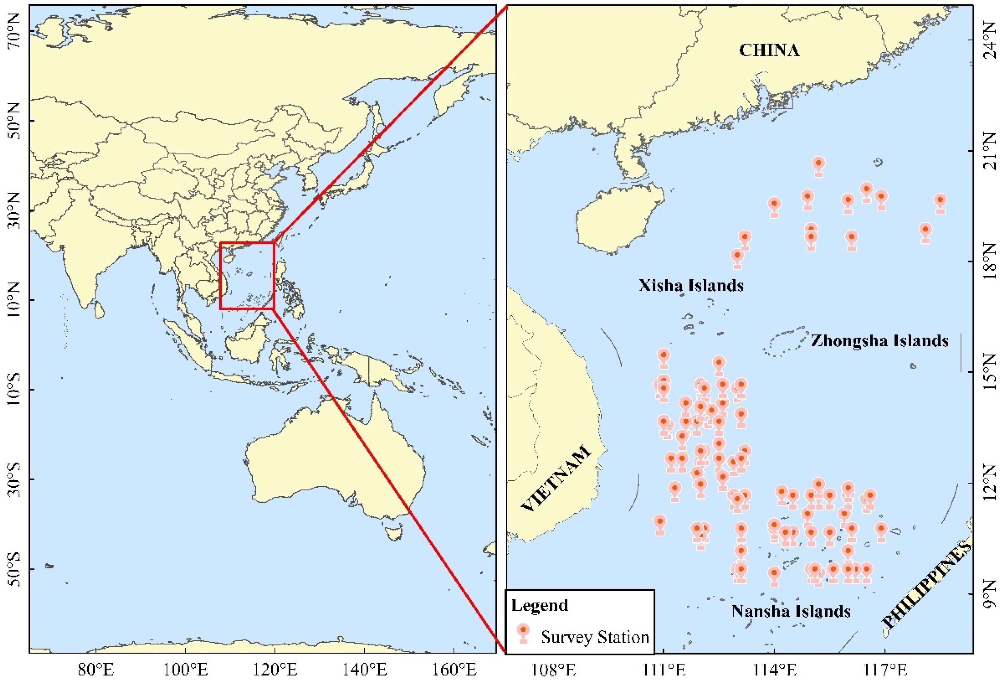
2.1. Fisheries and Environmental Data

Fisheries data were collected through an independent fisheries survey in the SCS conducted by the the South China Sea Fisheries Research Institute of the Chinese Academy of Fisheries Science from 2015–2019 (

Table 1. Survey sampling times.

Voyage	Time	Season
1	2015 April	Spring
2	2016 April	Spring
3	2017 April to May	Spring
4	2017 August to September	Summer
5	2018 May	Spring
6	2018 August to September	Summer
7	2019 May	Spring
8	2019 August to September	Summer

). Catch data, longitude/latitude, gea, speed and course were recorded for each station. Surveys were conducted in offshore SCS waters between 10–20° N and 110–118° E (Figure 1). The survey vessel, with weight 421 t and length 43.6 m, was equipped with metal halide fish lamps (1 kW). The net, ~281.60 m × 81.76 m, had maximum and minimum meshes of 35 mm and 20 mm, respectively, and weighed 2816 kg. When surveying, 300 lights were switched on at 19:00 for ~3 h every night. The catch data were logarithmically processed to satisfy a normal distribution when used.

As an environmental database, daily sea surface temperature (SST), sea surface temperature gradient (SSTG), Chlorophyll-a (Chl-a), sea surface height (SSH), sea surface salinity (SSS) and mixed layer depth (MLD) were used in this study. The units of SST, SSTG, Chl-a, SSH, SSS, and MLD were °C, °C, mg m⁻³, m, PSU, and m, respectively. The SST and Chl-a concentration data are from the Moderate Resolution Imaging Spectroradiometer (MODIS) on board the satellite Aqua platform and were obtained from National Oceanic and Atmosphere Administration (NOAA) (https://coastwatch.pfeg.noaa.gov/data.html, accessed on 26 March 2022). The data have a daily temporal resolution and a spatial resolution of 0.04°. The SSH, SSS, and MLD are provided by Copernicus Marine Environmental Monitoring Service (https://resources.marine.copernicus.eu/product-detail/GLOBAL_MULTIYEAR_PHY_001_030/INFORMATION, accessed on 27 March 2022). The data have a daily temporal resolution and a spatial resolution of 0.083°. In the product, the MLD is defined as a depth where the density increase compared to density at 10 m depth corresponds to a temperature decrease of 0.2 °C in local surface conditions (θ10 m, S10 m, P0 = 0 db, surface pressure). Based on maximum temperature gradient characteristic at the ocean temperature front, the SSTG is calculated using the following equation [27],

$$Gra{d}_{SST}=\sqrt{D_X{}^2+D_Y{}^2}$$

$$D_X=\frac{SST\left(i,j+1\right)-SST\left(i,j-1\right)}{2\Delta X}$$

$$D_Y=\frac{SST\left(i+1,j\right)-SST\left(i,j-1\right)}{2\Delta Y}$$

where $Gra{d}_{SST}$ is the sea surface temperature gradient; $D_X$ and $D_Y$ are the gradients of adjacent points in the $X$ and $Y$ directions, respectively; $\Delta X$ and $\Delta Y$ are the pixel spacing in the $X$ and $Y$ directions, respectively; and $i$ and $j$ denote the positions of pixel points on the image, respectively.

Since the spatial resolutions of each dataset are different they were re-sampled to fit the fishery data resolution. Daily values of environmental data were extracted from each pixel corresponding to the location of fishing activities by ArcGIS software (ESRI, Redlands, CA, USA).

2.2. Model Construction

2.2.1. GAM

GAM is a nonparametric extension of a generalized linear model (GLM) [28] which is more suitable for dealing with nonlinear problems. GAM focuses on exploring data nonparametrically to capture relationships between the marine environment and resource abundance [29]. To avoid excessive computation and over-fitting, the linear correlation between each explanatory variable is measured according to a Variance Inflation Factor (VIF) before GAM is performed. When VIF > 10, explanatory variables have a linear relationship with each other and should be removed from the model [30,31]. We used the R mgcv package to fit the GAM [32,33]. The general form the model can be written as:

$$g\left(\mu \right)=\beta +f_1\left(x_1\right)+f_2\left(x_2\right)+\cdots +f_i\left(x_i\right)+\epsilon$$

where $g\left(\mu \right)$ is the link function, which is the logarithm of Catch; $\beta$ is the intercept term; $f$ is a smooth function; $i$ is the number of predictor variables, and $\epsilon$ is an error term. The GAM procedure uses smoothing splines $s( )$.

2.2.2. HSI

The HSI model objectively estimates the suitable environmental range for a species to survive [34]. Assuming the sea area with the largest Catch is the sea area with the most abundant resources, it follows that the sea area with the least Catch is the sea area with the most impoverished resources; the former suitability index (SI) is set to 1 and the latter to 0 [35]. We derive SI using the following formula:

$$S{I}_a=\frac{Catc{h}_i-Catc{h}_{min}}{Catc{h}_{max}-Catc{h}_{min}}$$

where $S{I}_a$ is the SI of the environmental factor $a$; $Catc{h}_i$ is the catch at station $i$;$Catc{h}_{max}$ is the maximum catch at all stations in the voyage; $Cat{c}_{min}$ is the minimum catch at all stations in the voyage. We fit the relationship between environmental factors and SI by nonlinear regression and solved by R software. We calculated the integrated habitat index model using the Arithmetic Mean Method (AMM) and verified it with survey data [36]. The equation of our HSI model is:

$$HSI=\frac{1}{n}\left(S{I}_1+S{I}_2+\cdots S{I}_n\right)$$

where $S{I}_1$, $S{I}_2$, $\cdots S{I}_n$, are the predicted SI values on the fishing ground for each environmental factor; and n is the number of environmental factors in the HSI model. If the differences between the theoretical and actual value exceed 0.3, the forecast is considered to be accurate, and vice versa [37]. The HSI spatial distribution of each season was plotted, and the habitat area was calculated. The areas with HSI ≥ 0.6, HSI ≥ 0.8, 0.2 < HSI < 0.6, and HSI ≤ 0.2 were regarded as suitable, optimal, normal, and poor habitats, respectively, for A. thazard [38].

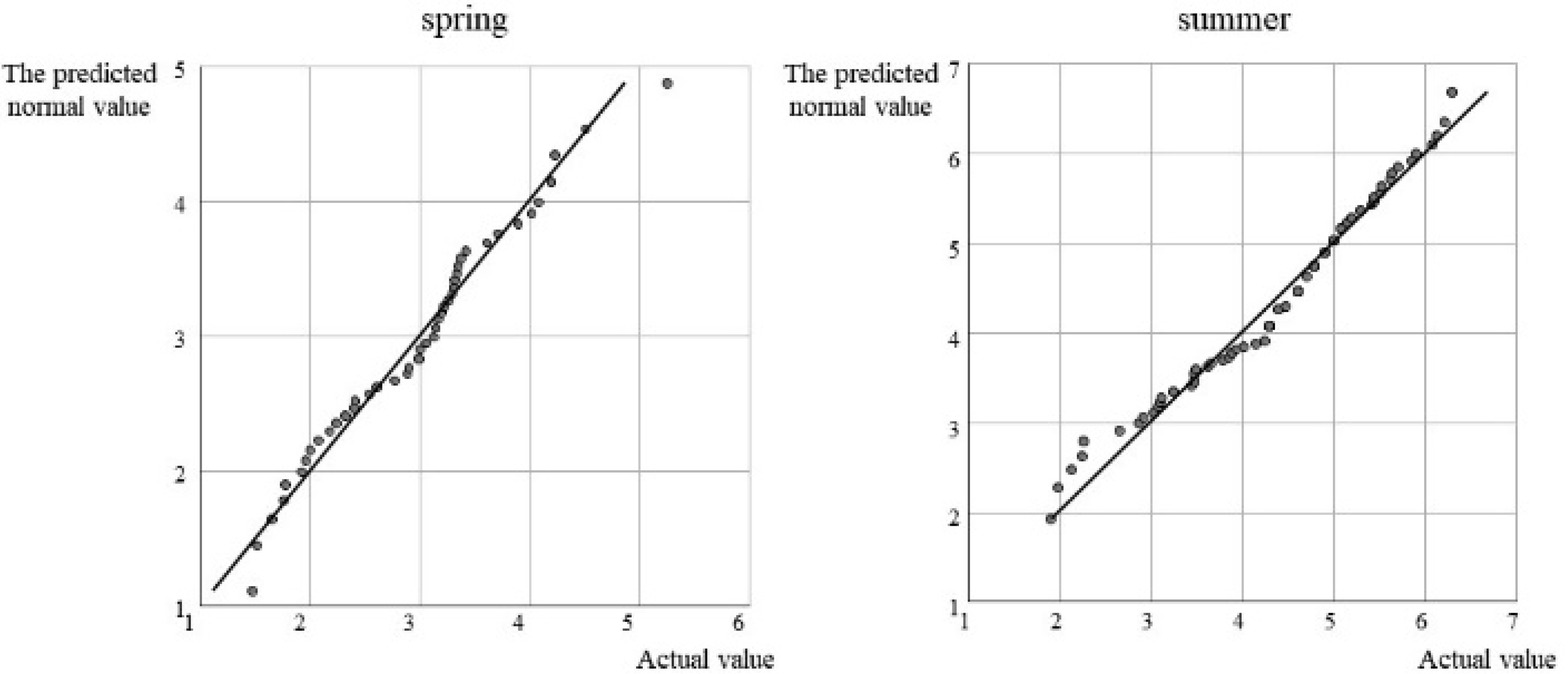
2.2.3. Cross Validation

The spring and summer optimal model were cross validated by dividing or partitioning the data into one portion used to calibrate the model (training data), and one portion to validate predictions, called the testing data. Huberty described a rule of thumb for determining the optimum partitioning of training and testing data for models, with the proportion of testing data being:

$$1/\left(1+\sqrt{\rho -1}\right)$$

where $\rho$ is the number of predictors. Other data are used as training data for model calculations.

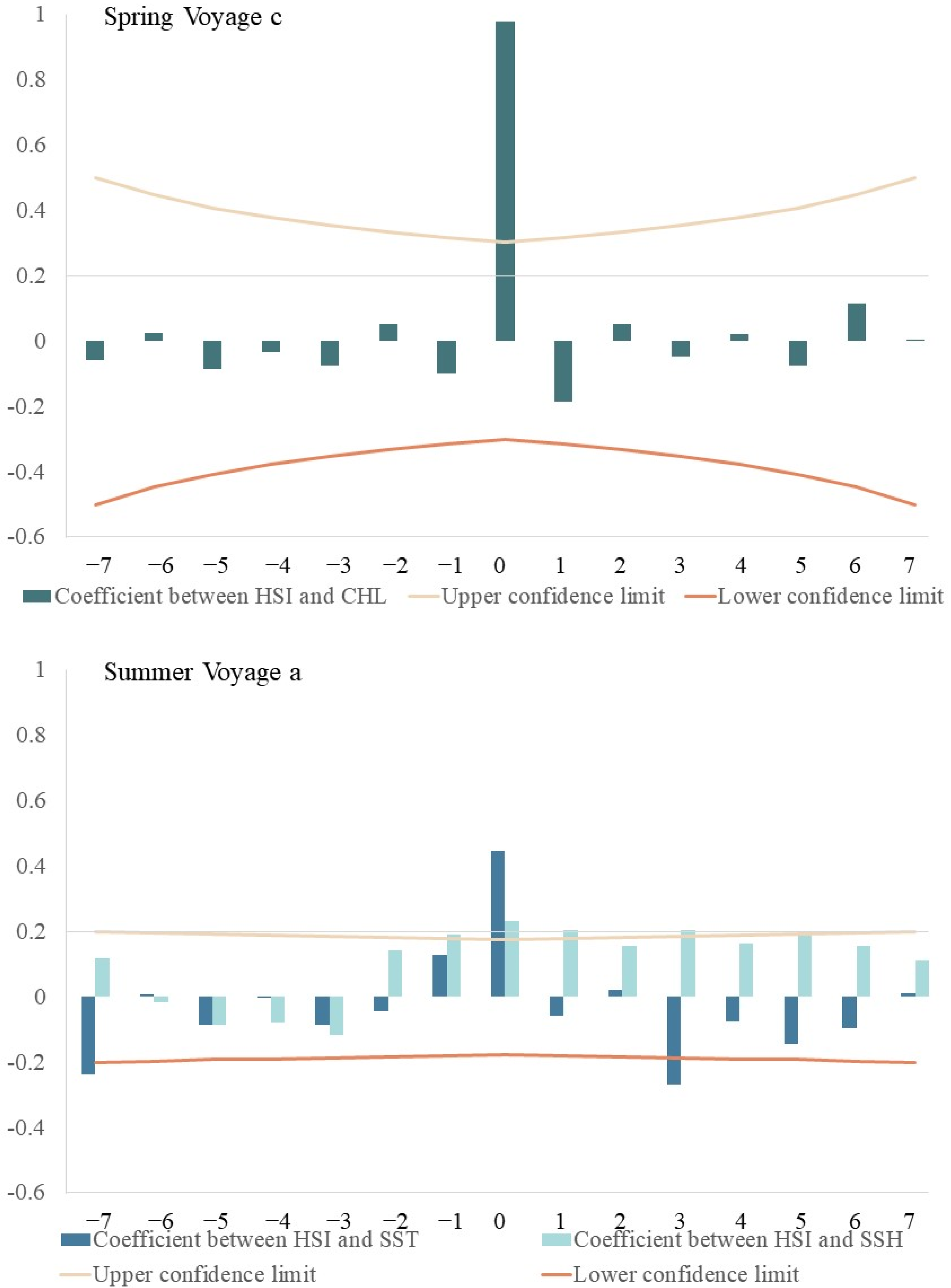
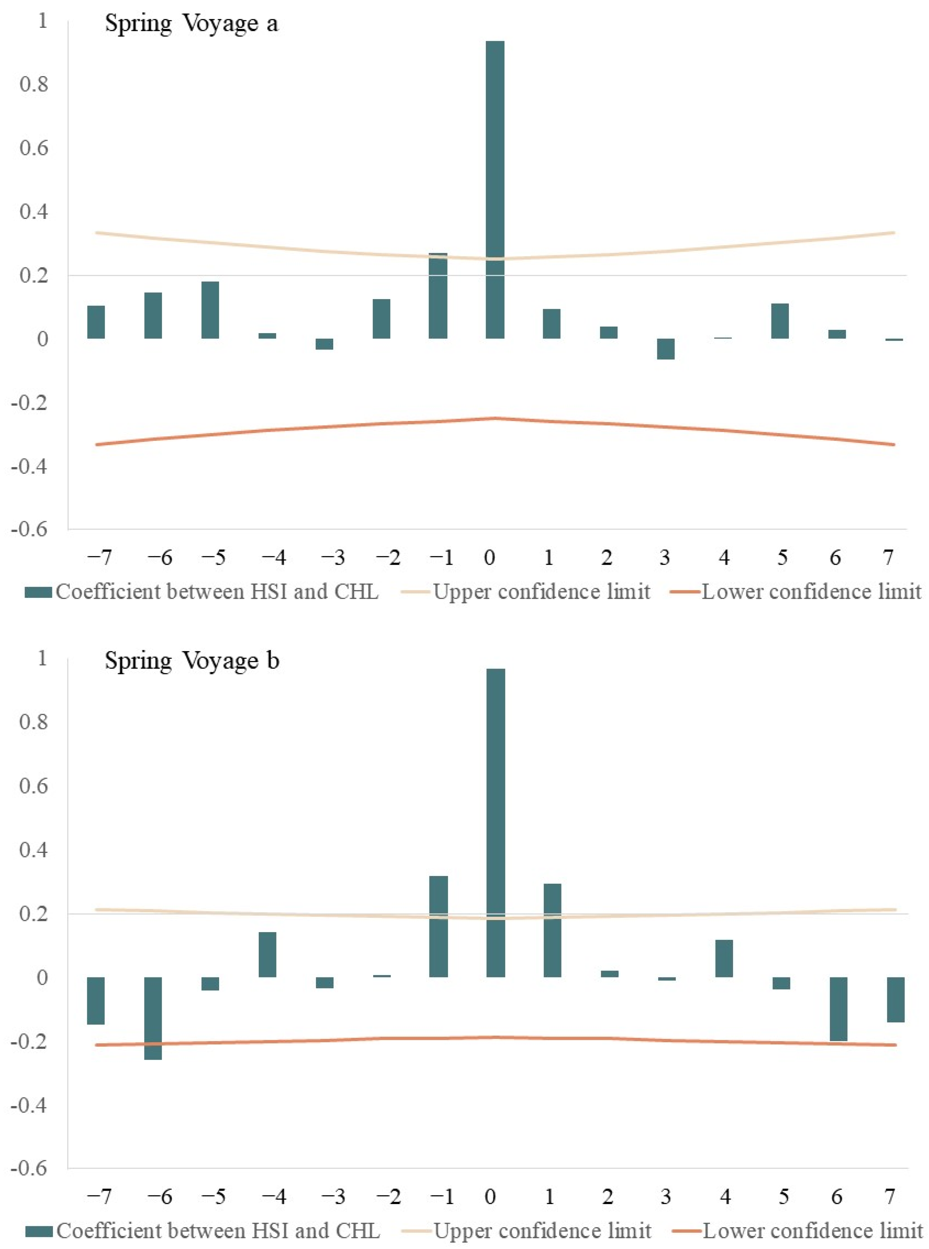
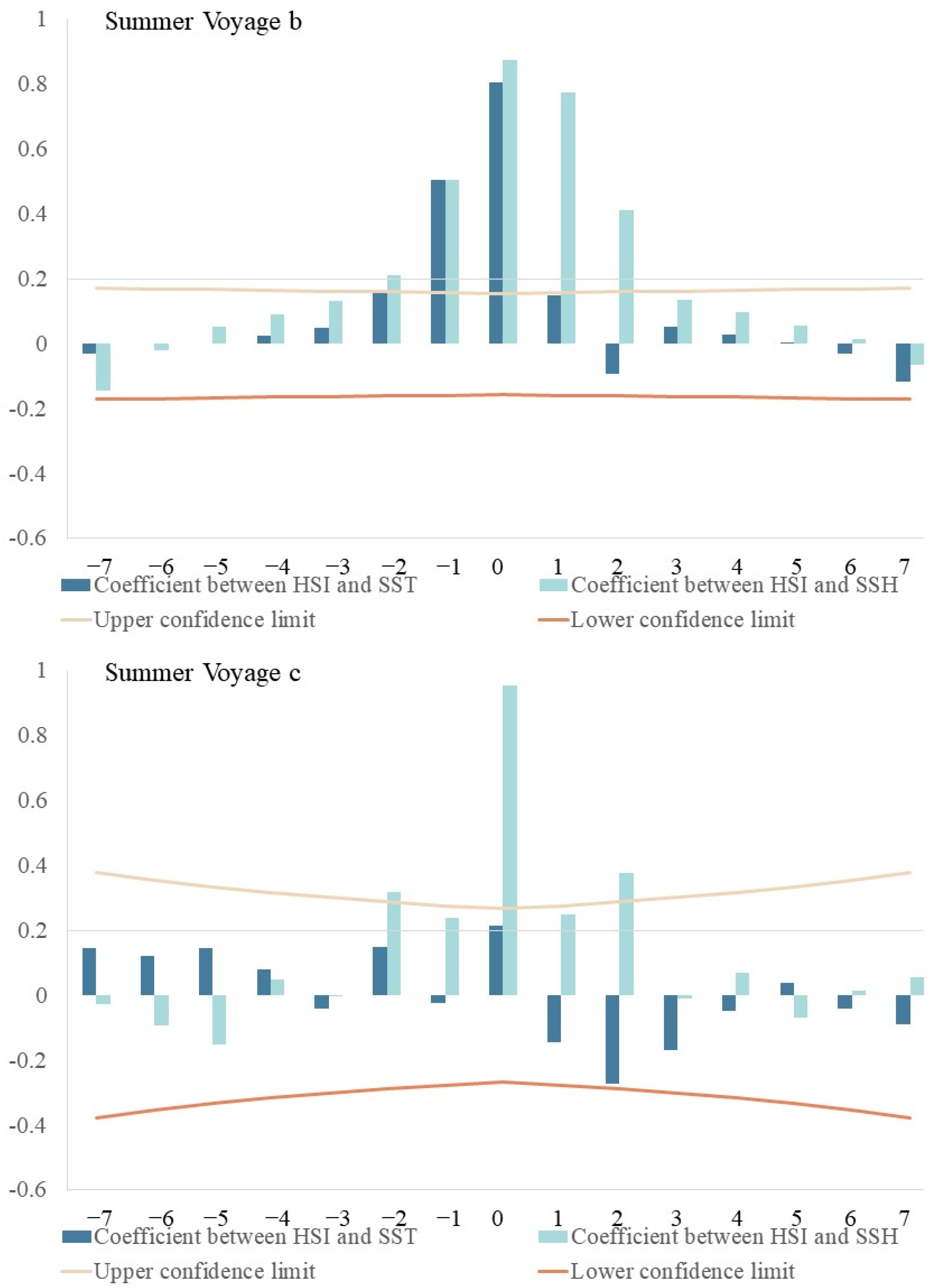
2.3. Time Delay Analysis

To determine if time-lagged effects of significant environmental factors existed on A. thazard habitat, spatiotemporal relationships between monthly average HSI values and environmental factors were further evaluated using cross-correlation plots.

3. Results

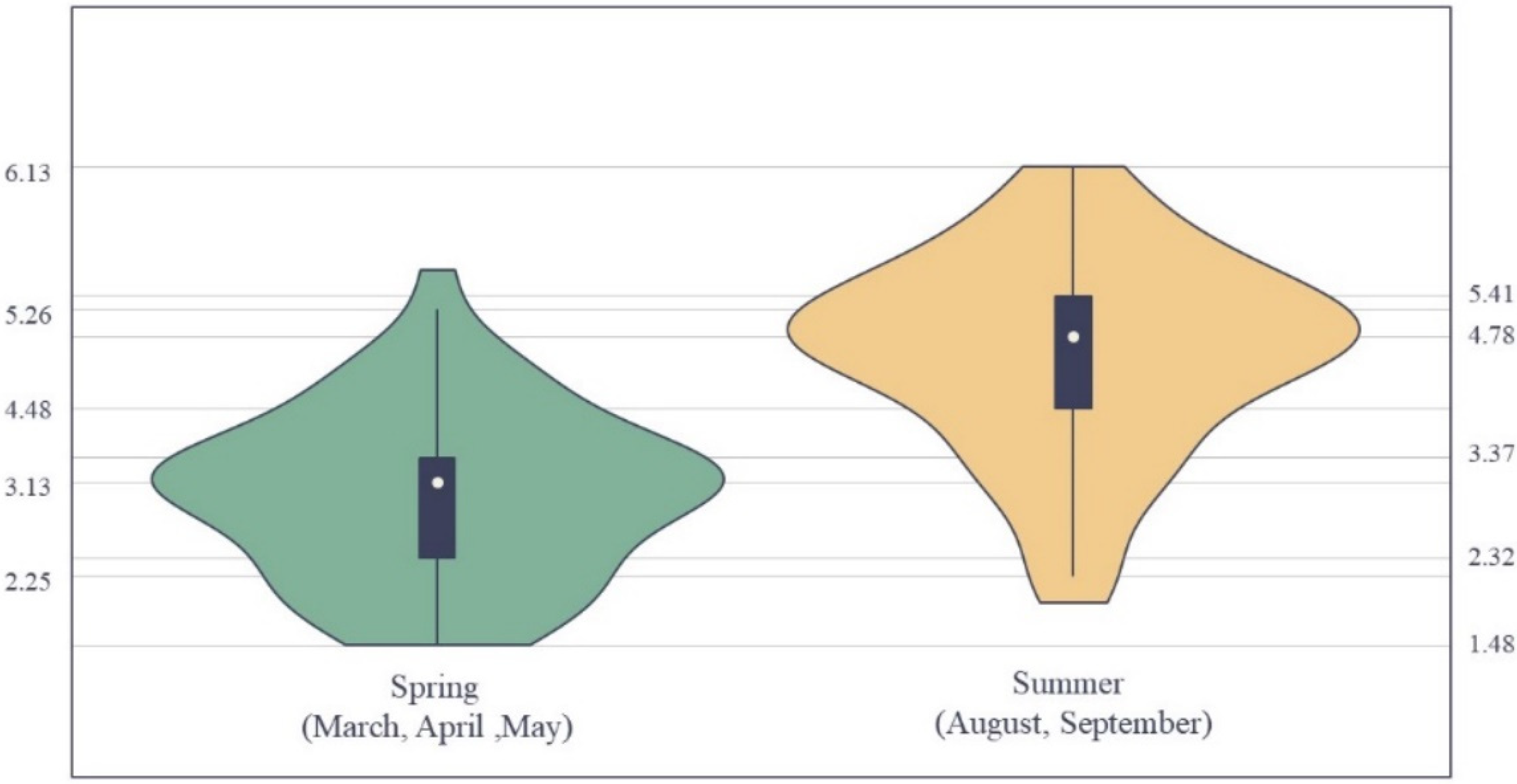
3.1. Catch Data Distribution

The overall distribution of the logarithmic catch data is presented in Figure 2. Lg (Catch) of A. thazard was high in summer, peaking at 6.13, with an upper quartile of 5.41, lower quartile of 4.48, and a minimum of 2.25 (Figure 2). Catch of A. thazard (lg) was low in spring, peaking at 5.26, with an upper quartile of 3.37, lower quartile of 2.32, and minimum of 1.48. Comparing the summer and spring kernel density distribution plots of A. thazard lg (Catch) the distribution of A. thazard lg (Catch) in summer peaks at ~4.78, and that in spring peaks at ~3.13. All maxima, upper and lower quartiles, and median values for A. thazard lg (Catch) in summer were higher than those in spring.

A normality test for A. thazard lg (Catch) reveals the lg (Catch) data points to basically form a straight line in the normal QQ-plot, indicating that lg (Catch) conforms to the normal distribution and satisfies the basic premise of GAM construction (Figure 3).

3.2. Environmental Factor Screening

Collinearity diagnostics tests of temporal and environmental variables reveal the VIF of all environmental factors to be <10, indicating no collinearity exists amongst them (

Table 2. Collinearity diagnostics tests of environmental variables.

Season	Month	SST	SSTG	Chl-a	MLD	SSS	SSH	Year
Spring	2.856	2.789	3.134	1.270	1.694	1.476	1.767	2.274
Summer	3.476	1.552	3.034	1.096	1.926	1.489	3.936	3.260

). Therefore, all environmental factors can be used in the GAM, which is constructed using complete subset regression, selecting the optimal combination of explanatory variables according to Mallows’ Cp and Adjusted R-square (

Table 3. Generalized additive models (GAMs) fitted to A. thazard Catch and analysis of deviance.

Season	GAM Expression	R-sq.(adj)	Deviance Explained	Scale Est	GCV	AIC	RMSE
Spring	(lg (Catch)) ~ factor(year)+s(SSTG)+s(Chl-a)+s(SSS)	0.347	46.90%	0.469	0.589	108.246	0.684
Summer	(lg (Catch)) ~ factor(month)+s(SST)+s(SSH)	0.267	33.60%	0.729	0.813	263.927	0.967

and

Table 4. Significance test results of explanatory variables.

Season	Significance Environmental Variables	Edf	Ref.df	F	p-Value
Spring	SSTG	1.002	1.003	1.779	0.190
	Chl-a	1.056	1.109	6.754	0.010 *
Summer	SSS	2.537	3.166	0.948	0.428
	SST	3.227	4.05	4.868	0.001 **
	SSH	5.114	6.208	2.272	0.042 *

* p < 0.01, a statistically significant difference. ** p < 0.001, a highly statistically significant difference.

). Four-fold cross-validation was used to evaluate the model; when the RMSE > 1, the model was deemed reasonable. Significant environmental variables (p ≤ 0.05) were different between spring and summer. In spring, the significant variable was Chl-a, while in summer they were SST and SSH.

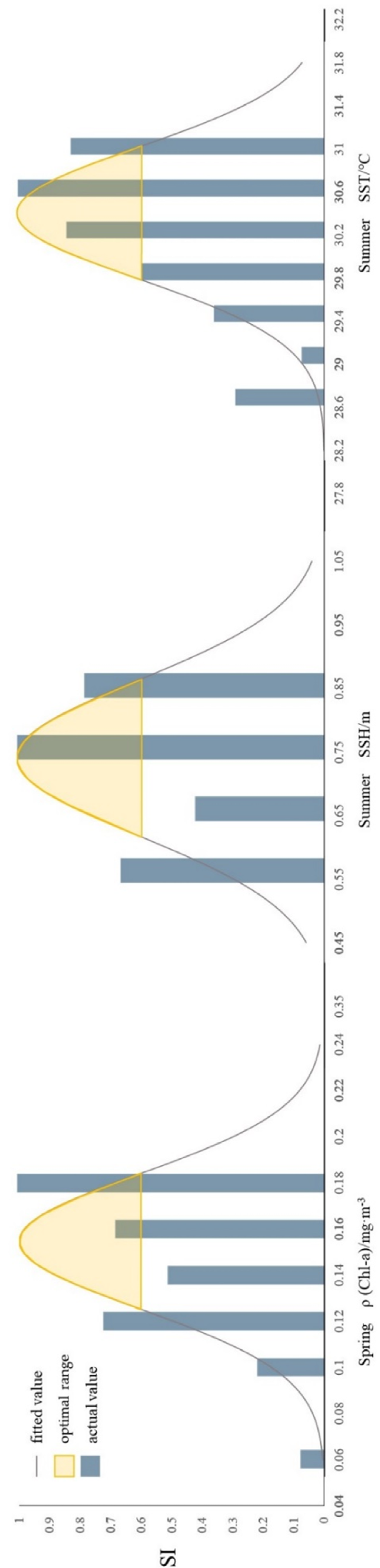
3.3. Analysis of HSI Model

We fitted the relationship between lg (Catch) and environmental factors that differed significantly between seasons (Chl-a, SST, SSH) using unary nonlinear regression (Figure 4,

Table 5. SI model for each environmental factor that differed significantly between spring and summer.

Season	Significance Environmental Factors	HSI Expression	F Value	p Value	R2
Spring	Chl-a	X2 = EXP(−587.708648 × (X1 − 0.154604)2)	12.927	0.007	0.618
Summer	SST	X2 = EXP(−1.345476 × (X1 − 30.405269)2)	41.905	0.000	0.840
	SSH	X2 = EXP(−33.704041 × (X1 − 0.741042)2)	11.467	0.020	0.696

), and calculated SI value for each significant environmental factor. The significance level of each function expression is p < 0.05. The HSI model is obtained using the arithmetic average method, and the model accuracy verified by the 0.3 standard (

Table 6. Areas of different habitat types in spring and summer.

HSI	Spring (Km2)	Summer (Km2)
0–0.2	394,776.800	653.551
0.2–0.4	361,754.100	11,669.310
0.4–0.6	170,262.900	604,546.100
0.6–0.8	74,041.410	217,699.200
0.8–1	10,061.910	179,244.800

), if the difference between the predicted value and the actual value is less than 0.3, the forecast is considered correct, otherwise, the forecast is considered wrong. In spring, the numbers of correct and incorrect forecasts were 47 and 0, respectively, and the model accuracy was 100%. In summer, the numbers of correct and incorrect forecasts were 72 and 28, respectively, and the model accuracy was 72%. The average model accuracy of both seasons was 86%. Therefore, the fit is reliable and precise. The most suitable value of significant environmental factors in each season was obtained when SI was close to 1, and the greatest range of values occurred when SI ≥ 0.6. The optimum Chl-a value in spring was 0.154604, with an approximate optimum range of 0.1252–0.1840; the optimum SST value in summer was 30.405269, with an approximate optimum range of 29.7892–31.0214; and the optimum SSH value in summer was 0.741042, with an approximate optimum range of 0.6178–0.8641 (Figure 4).

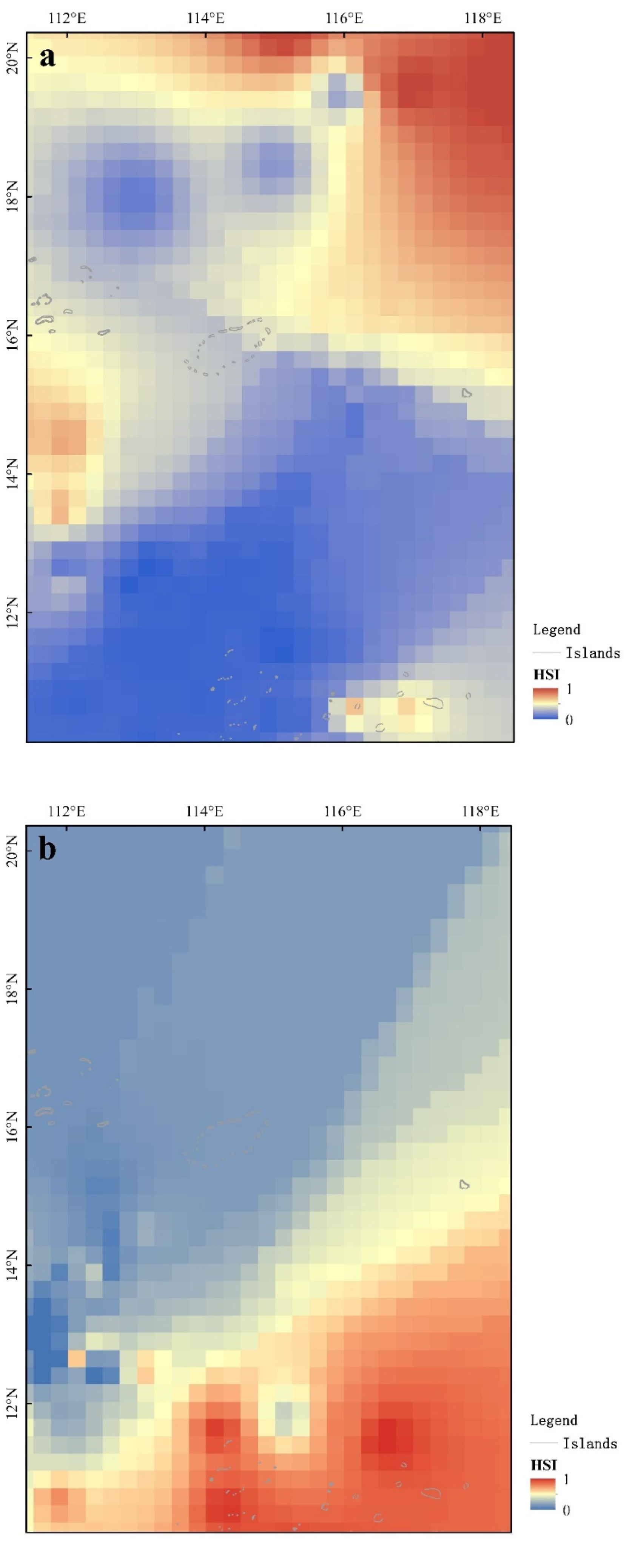
3.4. Habitat Variation

Mapping the A. thazard HSI distribution in spring and summer using ArcGIS 10.8 revealed suitable habitats to be mainly patchy (Figure 5). Suitable habitat in spring occurs mainly in northeastern sea areas, and in patches southwest of Paracel Islands near Vietnam and east of Nansha Islands, such as Renai Reef and Mischief Reef (Figure 5). Suitable habitats in summer occur mainly around Nansha Islands in southeastern waters, with patchy habi also found in southwestern waters near Vietnam. Additionally, compared with that in spring, the suitable habitat completely moved from the northeast areas to the southeast areas in summer, and the area of suitable habitat increased significantly in summer, and the SI of the entire sea area increased (Table 6).

3.5. Relationship between Significant Environmental Factors and Habitat Quality

Cross-correlation analysis revealed a significantly positive relationship between average HSI and Chl-a (Figure 6), with time-lags from 0–1 d during spring voyage 2, 0–6 d during spring voyage 3, and 0 d during spring voyage 4. The highest correlation coefficients (0.937, 0.967, 0.977) had close-to 0-day time-lags. Average HSI values and SST had time-lags from 3–6 d during summer voyage 1, 0–2 d during summer voyage 2, and 2 d in summer voyage 3. The highest correlation occurred at 0-d, 0-d, 2-d time-lags, with correlation coefficients of 0.447, 0.807, and −0.273, respectively. Average HSI and SSH had time-lags from 1–5 d during summer voyage 1, 0–2 d during summer voyage 2, and 0–2 d during summer voyage 3; the highest correlation coefficients (0.232, 0.874, 0.953) occurred with an approximately 0-d time-lag.

4. Discussion

March–May (spring) is the breeding date of A. thazard [25,39,40,41]. The effect of water temperature on fish is especially obvious during pre-oviposition and oviposition periods. Generally speaking, suitable temperature ranges for spawning are narrower than those for survival, with temperatures below or above these ranges limiting gonad development or maturation [42]. Rising water temperatures during spring would theoretically reduce the reproductive capacity of A. thazard in southern areas. Changed currents and high nutrient loadings in more northern waters might explain the migration of A. thazard to them because of their increased suitability for larval and juvenile growth [43]. During this time the southwest monsoon drives surface waters rich in nutrients and plankton northeast to the continental shelf and slope, providing suitable conditions for A. thazard larval growth and development [44,45].

From August–September (summer), the size of the A. thazard population experiencing spawning migration and reproduction increases rapidly, and larva and juveniles drifted to each distribution area with the current and monsoon [45]. Adult fish migrate to areas with abundant food and gain conditions [40]. Suitable habitat for A. thazard occurs mostly near the Nansha Islands from August to September (summer) (Figure 5). In the shallow waters of Nansha Islands, where the sun is high at noon, daylight hours are long, and water temperatures are high. Water currents in the SCS are complex from August to September. There are many islands and reefs around the Nansha Islands, and the water flow is affected by topographical obstacles. The Nansha Islands are located in the confluence of different flow systems and water masses, with the flow around the Nansha Islands also affected by terrain, creating many eddies [46,47]. The eddy tends to cause strong vertical movements of seawater, resulting in the bottom water surging upwards and the surface water sinking downwards. Movements of seawater can promote the mixing of seawater and bring high-nutrient subsurface water to the surface layer, which can boost plankton growth and increase the aggregation of prey organisms [48]. Thus, the Nansha Islands area is the important habitat of A. thazard (Figure 7).

An accurate and precise species abundance index (AI) is generally considered to be most important for fisheries forecasting and stock assessment, and represents the most important input for a fishery model. Catch AI, CPUE AI, and Effort AI are common indicators of resource abundance when building fishery models [49,50]. We use Catch AI to construct an HSI model. From the SI curve, we determine that catch data are closely related to environmental conditions. High catch data indicate that A. thazard is concentrated within a region, indicating that environmental conditions are conducive to its survival. Another important reason to use these catch data is that they were obtained during scientific investigation rather than from commercial fisheries. Not only do catch levels not affect fishing behavior, but fishery data are collected using standard gear and protocols over a long time period, at defined spatial and/or temporal scales. Thus, these data theoretically provide an unbiased estimate of fish population parameters [51]. In a study on the neon flying squid Ommastrephes bartramii, fishery models based on three AIs were compared, and results showed that for both simulated and real datasets, Catch AI was more accurate, consistent, and had better spatial representational ability at all spatial scales when compared with CPUE AI and Effort AI [52]. Accordingly, Catch AI-based fishery models are important tools for assessing the impacts of environmental change on marine species habitat, and provide a scientific basis for resource management.

Obvious seasonal and spatial variations exist in environmental conditions and habitat patterns for A. thazard. Favorable environmental conditions play an important role in regulating the range and distribution of suitable habitats. In fact, for habitats, environmental factors affecting habitat distribution of different species, regions, and seasons all differ [53]. When modeling fisheries, the fewer environmental variables used the better. Therefore, choosing fewer, more appropriate environmental variables can avoid overfitting and improve model interpretation. Common methods to statistically screen variables include stepwise regression (forward, backward, and forward–backward hybrid methods) and complete subset regression. In stepwise regression, each iteration can only follow the direction of the previous iteration [54]. However, complete subset regression can fit the possible combination models of all variables, and select the optimal model with variable combinations according to R-squared, Mallows’ Cp, Adjusted R-squared, AIC (Akaike Information Criterion), or other standards [55]. For accurate prediction of habitat distribution, the selection of appropriate environmental factors is important. For example, through stepwise regression, the most important environmental factors affecting the distribution of bigeye tuna (Thunnus obesus) in southern Java–Bali waters were SST, SSC, and SSHD [56], but off western Guangdong, water depth had the greatest impact on the distribution of Japanese scad Decapterus maruadsi [38]. Although variable screening through stepwise regression can establish a good model, it cannot guarantee that the constructed model is the best, because not every possible model is evaluated. To overcome this problem, we use complete subset regression to screen variables. Compared with stepwise regression, complete subset regression is computationally more complex, but it ensures that the selected combination of variables is optimal. According to Mallows’ Cp and Adjusted R-squared, we selected the best model, environmental factors were statistically (objectively) screened, and we obtained a simple and effective model.

Statistically optimal combination of catch variables and significant environmental variables can be obtained through full subset regression methods. However, this does not mean that variables that are not screened out have no effect on habitat. For example, some studies showed that MLD had an important effect on tuna habitat distribution [57]. In our study, the environmental data were all derived from satellite remote sensing, which is the secondary product of remote sensing data such as remote sensing images and radar data, and has certain limitations. Water depth, water turbidity, clouds, and reanalysis models will all affect the quality of secondary product, which in turn will affect the results of variable screening and model construction [58]. Compared with traditional walk-around sampling and monitoring, remote sensing satellite have many irreplaceable advantages in constructing habitat models, such as quick access of information, consecutive data, and ability to cover large areas. Our study area is mainly located in the sea beyond the 200 m depth, where the water is relatively high-transparent and has relatively little influence on the inversion results of satellite remote sensing, enabling it to construct a credible habitat model.

5. Conclusions

We reported the spatial and temporal distribution of A. thazard habitat in the South China Sea for the spring and summer months through an analysis of independent scientific survey and remote sensing data (SST, SSTG, Chl-a, SSH, SSS and MLD). Of all environmental variables used in modeling, Chl-a during spring had the greatest impact on the distribution of A. thazard, while SST and SSH had the greatest effect in summer. The habitat pattern of A. thazard differs seasonally and spatially. Favorable environmental conditions play an important role in regulating the range and location of suitable habitats (HSI ≥ 0.6). In future work, data collection in autumn and winter should be strengthened, and complete time series data should be accumulated to understand the life history of the species.

References

1. Xu, L.; Wang, X.; Van Damme, K.; Huang, D.; Li, Y.; Wang, L.; Ning, J.; Du, F. Assessment of fish diversity in the South China Sea using DNA taxonomy. Fish. Res. 2021, 233, 105771. [Google Scholar] [CrossRef]
2. Pauly, D.; Zeller, D. Catch reconstructions reveal that global marine fisheries catches are higher than reported and declining. Nat. Commun. 2016, 7, 10244. [Google Scholar] [CrossRef] [PubMed]
3. Cao, L.; Chen, Y.; Dong, S.; Hanson, A.; Huang, B.; Leadbitter, D.; Little, D.C.; Pikitch, E.K.; Qiu, Y.; de Mitcheson, Y.S.; et al. Opportunity for marine fisheries reform in China. Proc. Natl. Acad. Sci. USA 2017, 114, 435–442. [Google Scholar] [CrossRef]
4. Uchida, R.N. Synopsis of Biological Data on Frigate Tuna, Auxis Thazard, and Bullet Tuna, A. rochei. In FAO Fisheries Synopsis; US Department of Commerce, National Oceanic and Atmospheric Administration, National Marine Fisheries Service: Silver Spring, MD, USA, 1981; 124p. [Google Scholar]
5. Zhang, J.; Qiu, Y.; Chen, Z.; Zhang, P.; Zhang, K.; Fan, J.; Chen, G.; Cai, Y.; Sun, M. Advances in pelagic fishery resources survey and assessment in open South China Sea. S. China Fish. Sci. 2018, 14, 118–127. [Google Scholar]
6. Petitgas, P.; Doray, M.; Huret, M.; Massé, J.; Woillez, M. Modelling the variability in fish spatial distributions over time with empirical orthogonal functions: Anchovy in the Bay of Biscay. ICES J. Mar. Sci. 2014, 71, 2379–2389. [Google Scholar] [CrossRef]
7. Valavanis, V.D.; Pierce, G.J.; Zuur, A.F.; Andreas, P.; Anatoly, S.; Isidora, K.; Wang, J. Modelling of essential fish habitat based on remote sensing, spatial analysis and GIS. Hydrobiologia 2008, 612, 5–20. [Google Scholar] [CrossRef]
8. US Fish and Wildlife Service (USFWS) Standards for the Development of Habitat Suitability Index Models; US Fish and Wildlife Service, Division of Ecological Service: Washington, DC, USA, 1981.
9. Yen, K.W.; Lu, H.J.; Chang, Y.; Lee, M.A. Using remote-sensing data to detect habitat suitability for yellowfin tuna in the Western and Central Pacific Ocean. Int. J. Remote Sens. 2012, 33, 7507–7522. [Google Scholar] [CrossRef]
10. Chen, X.; Li, G.; Feng, B.; Tian, S.Q. Habitat suitability index of Chub mackerel (Scomber japonicus) from July to September in the East China Sea. J. Oceanogr. 2009, 65, 93–102. [Google Scholar] [CrossRef]
11. Jones, M.C.; Dye, S.R.; Pinnegar, J.K.; Warren, R.; Cheung, W.W.L. Modelling commercial fish distributions: Prediction and assessment using different approaches. Ecol. Model. 2012, 225, 133–145. [Google Scholar] [CrossRef]
12. Li, G.; Chen, X.; Lei, L.; Guang, W.J. Distribution of hotspots of chub mackerel based on remote-sensing data in coastal waters of China. Int. J. Remote Sens. 2014, 35, 4399–4421. [Google Scholar] [CrossRef]
13. Li, G.; Cao, J.; Zou, X.; Chen, X.J.; Runnebaum, J. Modeling habitat suitability index for Chilean jack mackerel (Trachurus murphyi) in the South East Pacific. Fish. Res. 2016, 178, 47–60. [Google Scholar] [CrossRef]
14. Engel, D.W.; Thayer, G.W.; Evans, D.W. Linkages between fishery habitat quality, stressors, and fishery populations. Environ. Sci. Policy 1999, 2, 465–475. [Google Scholar] [CrossRef]
15. Agenbag, J.J.; Richardson, A.J.; Demarcq, H.; Fréon, P.; Weeks, S.; Shillington, F.A. Estimating environmental preferences of South African pelagic fish species using catch size-and remote sensing data. Prog. Oceanogr. 2003, 59, 275–300. [Google Scholar] [CrossRef]
16. Bacha, M.; Jeyid, M.A.; Vantrepotte, V.; Dessailly, D.; Amara, R. Environmental effects on the spatio-temporal patterns of abundance and distribution of Sardina pilchardus and sardinella off the Mauritanian coast (North-West Africa). Fish. Oceanogr. 2017, 26, 282–298. [Google Scholar] [CrossRef]
17. Hastie, T.J.; Tibshirani, R.J. Generalized Additive Models. Stat. Sci. 1986, 1, 297–318. [Google Scholar] [CrossRef]
18. Jegatheesan, J.; Zakaria, Z. Stress analysis on pressure vessel. Environ. Ecosyst. Sci. 2018, 2, 53–57. [Google Scholar] [CrossRef]
19. Stoner, A.W.; Manderson, J.P.; Pessutti, J.P. Spatially explicit analysis of estuarine habitat for juvenile winter flounder: Combining generalized additive models and geographic information systems. Mar. Ecol. Prog. Ser. 2001, 213, 253–271. [Google Scholar] [CrossRef]
20. Venables, W.N.; Dichmont, C.M. GLMs, GAMs and GLMMs: An overview of theory for applications in fisheries research. Fish. Res. 2004, 70, 319–337. [Google Scholar] [CrossRef]
21. Syamsuddin, M.L.; Saitoh, S.I.; Hirawake, T.; Bachri, S.H.; Agung, B. Effects of El Niño–Southern Oscillation events on catches of bigeye tuna (Thunnus obesus) in the eastern Indian Ocean off Java. Fish. Bull. 2013, 111, 175–188. [Google Scholar] [CrossRef]
22. Cornic, M.; Rooker, J.R. Influence of oceanographic conditions on the distribution and abundance of blackfin tuna (Thunnus atlanticus) larvae in the Gulf of Mexico. Fish. Res. 2018, 201, 1–10. [Google Scholar] [CrossRef]
23. Li, M.; Zhang, P.; Li, Y.; Chen, S.; Zhang, K.; Kong, X.; Chen, Z. Population genetic structure and genetic diversity of frigate tuna ( Auxis thazard) in the South China Sea. S. China Fish. Sci. 2015, 11, 82–89. [Google Scholar]
24. Kong, X.; Jiang, Y.; Gong, Y.; Chen, Z.; Zhang, J.; Fang, J. A preliminary study on fishery biology of Ceratoscopelus warmingii in the central and northern South China Sea. S. China Fish. Sci. 2016, 12, 117–124. [Google Scholar]
25. Lu, Z.; Yan, Y.; Dai, Q. Biology of Resource of Auxis thazard in the Minzhong and Mindong Fishing Ground. J. Oceanogr. Taiwan Strait 1992, 11, 251–256. [Google Scholar]
26. Zhou, X.; Fan, J.; Yu, J.; Xu, S.; Cai, Y.; Chen, Z. Geostatistics-based study on spatial-temporal distribution of Auxis thazard in South China Sea. S. China Fish. Sci. 2022, 18, 1–8. [Google Scholar] [CrossRef]
27. Jing, Z.; Qi, Y.; Du, Y.; Zhang, S.; Xie, L. Summer upwelling and thermal fronts in the northwestern South China Sea: Observational analysis of two mesoscale mapping surveys. J. Geophys. Res. Ocean. 2015, 120, 1993–2006. [Google Scholar] [CrossRef]
28. Potts, S.E.; Rose, K.A. Evaluation of GLM and GAM for estimating population indices from fishery independent surveys. Fish. Res. 2018, 208, 167–178. [Google Scholar] [CrossRef]
29. Sudhakaran, M.; Ramamoorthy, D.; Savitha, V.; Balamurugan, S. Assessment of trace elements and its influence on physico-chemical and biological properties in coastal agroecosystem soil, Puducherry region. Geol. Ecol. Landsc. 2018, 2, 169–176. [Google Scholar] [CrossRef]
30. Heiberger, R.M.; Holland, B. Statistical Analysis and Data Display an Intermediate Course with Examples in R; Springer: Berlin/Heidelberg, Germany, 2015. [Google Scholar]
31. Kutner, M.H.; Christopher, J.N.; John, N.; William, L. Applied Linear Statistical Models; McGraw-Hill Irwin: New York, NY, USA, 2005. [Google Scholar]
32. Wood, S.N. Stable and efficient multiple smoothing parameter estimation for generalized additive models. J. Am. Stat. Assoc. 2004, 99, 673–686. [Google Scholar] [CrossRef]
33. Wood, S.N. Fast stable restricted maximum likelihood and marginal likelihood estimation of semiparametric generalized linear models. J. R. Stat. Soc. Ser. B 2011, 73, 3–36. [Google Scholar] [CrossRef]
34. Wakeley, J.S. A method to create simplified versions of existing habitat suitability index (HSI) models. Environ. Manag. 1988, 12, 79–83. [Google Scholar] [CrossRef]
35. Mohri, M.; Nishida, T. Seasonal change in bigeye tuna fishing areas in relation to the oceanographic parameters in the Indian Ocean. J. Natl. Fish. Univ. 1999, 47, 43–54. [Google Scholar]
36. Yu, W.; Yi, Q.; Chen, X.; Chen, Y. Modelling the effects of climate variability on habitat suitability of jumbo flying squid, Dosidicus gigas, in the Southeast Pacific Ocean off Peru. ICES J. Mar. Sci. 2016, 73, 239–249. [Google Scholar] [CrossRef]
37. Gao, F.; Chen, X.; Fan, J.; Lin, L.; Guang, W. Implementation and verification of intelligent fishing ground forecasting of Illex argentinus in the Southwest Atlantic. J. Shanghai Ocean. Univ. 2011, 20, 754–758. [Google Scholar]
38. Yu, J.; Liu, Z.; Chen, P.; Yao, L. Environmental factors affecting the spatiotemporal distribution of Decapterus maruadsi in the western Guangdong waters, China. Appl. Ecol. Environ. Res. 2019, 17, 8485–8499. [Google Scholar] [CrossRef]
39. Ghosh, S.; Sivadas, M.; Abdussamad, E.M.; Rohit, P.; Koya, K.P.S.; Joshi, K.K.; Chellappan, A.; Margaret Muthu Rathinam, A.; Prakasan, D.; Sebastine, M. Fishery, population dynamics and stock structure of frigate tuna Auxis thazard (Lacepede, 1800) exploited from Indian waters. Indian J. Fish. 2012, 59, 95–100. [Google Scholar]
40. Lu, Z.; Dai, Q.; Yan, Y. Growth and Mortality of Auxis thazard in the Taiwan Strait and its Adjacent Sea. J. Fish. China 1991, 15, 228–235. [Google Scholar]
41. Zhang, R. The distribution and spawning period of juveniles and juveniles of three tuna species (bonito, yellowfin tuna, and tuna) in the South China Sea. ACTA Oceanol. Sin. 1983, 5, 368–375. [Google Scholar]
42. Chen, X.J.; Liu, B.L. Biology of Fishery Resources; Science Press: China, Beijing, 2017. [Google Scholar]
43. King, M. Fisheries Biology, Assessment and Management; Blackwell Publishing: Oxford, UK, 2013. [Google Scholar]
44. Liu, K.; Chao, S.; Shaw, P.; Gong, G.; Chen, C.; Tang, T. Monsoon-forced chlorophyll distribution and primary production in the South China Sea: Observations and a numerical study. Deep Sea Res. Part I Oceanogr. Res. Pap. 2002, 49, 1387–1412. [Google Scholar] [CrossRef]
45. Wang, B.; Huang, F.; Wu, Z.; Yang, J.; Fu, X.; Kikuchi, K. Multi-scale climate variability of the South China Sea monsoon: A review. Dyn. Atmos. Ocean. 2009, 47, 15–37. [Google Scholar] [CrossRef]
46. Liu, Z.; Gan, J. Three-dimensional pathways of water masses in the South China Sea: A modeling study. J. Geophys. Res. Ocean. 2017, 122, 6039–6054. [Google Scholar] [CrossRef]
47. Fang, W.; Guo, Z.; Huang, Y. A study of circulation observations in the southern South China Sea marine area. Chin. Sci. Bull. 1997, 42, 2264–2271. [Google Scholar]
48. Chen, X.J. Fisheries Resources and Fishery Science; China Ocean Press: China, Beijing, 2004. [Google Scholar]
49. Francis, R.I.C.C. Data weighting in statistical fisheries stock assessment models. Can. J. Fish. Aquat. Sci. 2011, 68, 1124–1138. [Google Scholar] [CrossRef]
50. Methot, R.D., Jr.; Tromble, G.R.; Lambert, D.M.; Greene, K.E. Implementing a science-based system for preventing overfishing and guiding sustainable fisheries in the United States. ICES J. Mar. Sci. 2014, 71, 183–194. [Google Scholar] [CrossRef]
51. Stelzenmüller, V.; Ehrich, S.; Zauke, G.P. Impact of additional small-scale survey data on the geostatistical analyses of demersal fish species in the North Sea. Sci. Mar. 2005, 69, 587–602. [Google Scholar]
52. Wang, J.; Boenish, R.; Chen, X.; Tian, S.; Zhu, Z. The effects of spatiotemporal scale on commercial fishery abundance index suitability. ICES J. Mar. Sci. 2021, 78, 2506–2517. [Google Scholar] [CrossRef]
53. Doligez, B.; Boulinier, T. Habitat Selection and Habitat Suitability Preferences. J. Wildl. Manag. 2008, 5, 1810–1830. [Google Scholar]
54. Jennrich, R.I.; Sampson, P.F. Application of stepwise regression to non-linear estimation. Technometrics 1968, 10, 63–72. [Google Scholar] [CrossRef]
55. Zhang, Z. Variable selection with stepwise and best subset approaches. Ann. Transl. Med. 2016, 4, 136. [Google Scholar] [CrossRef] [PubMed]
56. Setiawati, M.D.; Sambah, A.B.; Miura, F.; Tanaka, T.; As-Syakur, A.R. Characterization of bigeye tuna habitat in the Southern Waters off Java–Bali using remote sensing data. Adv. Space Res. 2015, 55, 732–746. [Google Scholar] [CrossRef]
57. Arrizabalaga, H.; Dufour, F.; Kell, L.; Merino, G.; Ibaibarriaga, L.; Chust, G.; Irigoien, X.; Santiago, J.; Murua, H.; Fraile, I.; et al. Global habitat preferences of commercially valuable tuna. Deep Sea Res. Part II Top. Stud. Oceanogr. 2015, 113, 102–112. [Google Scholar] [CrossRef]
58. Qin, H.; Chen, G.; Wang, W.; Wang, D.; Zeng, L. Validation and application of MODIS-derived SST in the South China Sea. Int. J. Remote Sens. 2014, 35, 4315–4328. [Google Scholar] [CrossRef]
Figure 1. Spatial distribution of survey stations for A. thazard in the South China Sea, spring to summer, 2015–2019. Inset with red rectangular box marks the study area.
Fishes 07 00218 g001
Figure 2. Violin plot of lg (Catch) distribution of A. thazard for spring and summer.
Fishes 07 00218 g002
Figure 3. QQ-plot of A. thazard lg (Catch) in spring and summer.
Fishes 07 00218 g003
Figure 4. Seasonal fitted suitability index (SI) curves inferred from associations between fishing effort and Chlorophyll-a (Chl-a) concentration, sea surface height (SSH), and sea surface temperature (SST), spring to summer, 2015–2019.
Fishes 07 00218 g004
Figure 5. Distribution of A. thazard HSI in spring and summer, South China Sea: (a) Distribution of A. thazard HSI in spring; (b) Distribution of A. thazard HSI in summer.
Fishes 07 00218 g005
Figure 6. Cross-correlation coefficients between average HSI and environmental factors for Auxis thazard in the South China Sea. Spring Voyage a, b, c, which are voyages 2, 3, and 5 in Table 1, Summer Voyage a, b, c, which are voyages 4, 6, and 8 in Table 1.
Fishes 07 00218 g006aFishes 07 00218 g006bFishes 07 00218 g006c
Figure 7. Environment impacts the habitat of A. thazard in summer.
Fishes 07 00218 g007