Fish Face Identification Based on Rotated Object Detection: Dataset and Exploration

Abstract

At present, fish farming still uses manual identification methods. With the rapid development of deep learning, the application of computer vision in agriculture and farming to achieve agricultural intelligence has become a current research hotspot. We explored the use of facial recognition in fish. We collected and produced a fish identification dataset with 3412 images and a fish object detection dataset with 2320 images. A rotating box is proposed to detect fish, which avoids the problem where the traditional object detection produces a large number of redundant regions and affects the recognition accuracy. A self-SE module and a fish face recognition network (FFRNet) are proposed to implement the fish face identification task. The experiments proved that our model has an accuracy rate of over 90% and an FPS of 200.

1. Introduction

Aquatic products are rich in protein and amino acids, which can effectively meet the nutritional needs of people, and are gradually being favored by people because of their fresh and tender taste [1]. Therefore, people’s demand for aquatic products is also increasing year by year. Taking China as an example, the total amount of fishery products in 2019 was 50.79 million tons, an increase of 1.76% compared with 2018. At the same time, excessive fishing may lead to the deterioration of the marine ecological environment. Thus, environmental and ecological protection is an important issue for society and countries at present. In the future, the fishery industry should aim to reduce marine fishing to protect the ecological environment, and increase fishery breeding. However, with the increase in aquiculture and the expansion of the aquiculture area, the economic loss caused by diseases, improper feeding and other problems is increasing year by year [2]. Due to the complex water environment, electronic equipment in the water is easily affected by moisture and other factors. Compared with animal husbandry, fishery aquaculture is more traditional and backward. Identity recognition is the basis for the informationization and interconnection of the breeding industry. It can effectively improve the informationization of the breeding industry, record animal growth information, promote the exchange of breeding experiences and information, avoid the loss of breeding and sales caused by information occlusion and improve the value of the industry. At the same time, identity recognition is the premise of intelligent disease detection and early warning when breeding animals. In the intelligent detection of animal diseases and abnormal behaviors by computer vision methods, accurate positioning and early warning of animals can be carried out through identity identification. The identification of animals can effectively improve the intelligence of the industry. In disease detection and early warning, diseases and other information can be effectively recorded according to identity information to avoid the expansion of losses.

At present, the mainstream method of identity recognition in breeding is still the use of radio frequency identification (RFID) technology. In livestock breeding, RFID chips are usually embedded in the ears of pigs and cows, and the identity is recognized by different card readers in breeding circles [3]. This method is widely used because of its high recognition rate and low technical threshold. However, RFID requires artificial embedding of chips in animals. In small animals, such as chickens and ducks, a large number of chips may increase the breeding cost and consume significant human costs. Therefore, RFID technology has certain limitations in the realization of identity recognition in the breeding industry. Fish are usually smaller, and their breeding density is high. When embedding RFID chips, a high manpower cost is required because the water may interfere with the radio signal precision. Moreover, the water contains a lot of miscellaneous bacteria, so the embedded chip may damage the fish skin, cause fish death caused by bacterial infection or affect the normal swimming behavior of fish [4]. Therefore, RFID chips are not suitable for large-scale fishery breeding, which leads to the failure of identity recognition in fishery breeding and affects the development of intelligent information in the fishery industry.

In recent years, with the rapid development of deep learning, excellent solutions have been obtained for computer vision tasks [5]. Classification and recognition tasks are an important branch of computer vision tasks, and classification and recognition methods based on deep learning methods have achieved extremely high accuracy [6]. At present, they have been widely used in people’s real life, such as Alipay’s mobile payment through face recognition, stations’ initial detection of people entering and leaving the station through face recognition and ID cards, and automatic driving, which greatly facilitates people’s lives [7]. For example, in classification tasks, Howard A et al. proposed efficient lightweight networks such as MobilenetV1, MobilenetV2 and MobilenetV3 [8,9,10]. These networks reduce the number of parameters by deep separable convolution. K Han et al. proposed GhostNet, which generates more features using fewer parameters without changing the output feature map [11]. M Tan searched for a block architecture to replace the bottleneck structure based on MobileNetV2 [12]. For object detection tasks, Redmon J et al. proposed YOLOv1, YOLOv2, YOLOv3, YOLOv4, etc., to achieve extremely high detection fluency [13,14,15,16]. Zhou X proposed CenterNet, which first detects key points by prioritizing them and later obtains relevant attributes by regression [17]. Tan M et al. proposed the EfficientDet network, which replaces ResNet with a continuous convolutional downsampling layer, effectively improving detection efficiency and accuracy [18]. Jiang Y et al. proposed a new method called Rotational Region CNN for detecting text in arbitrary orientations. They extracted merged features using text boxes extracted by RPN and used these features to predict text and non-text scores, axis-aligned boxes and skewed minimum area boxes. Their work contributed significantly to the later application of rotated boxes to target detection [19]. Ding J et al. proposed the Rol Transformer for object detection in aerial images. The RoI Transformer is a three-stage detection model consisting mainly of RRoI Leaner and RRoI Wrapping, the two components. The core idea is to convert the horizontal anchor frame HRoI of the RPN output into a rotational anchor frame RRoI; therefore, an accurate RRoI is obtained without increasing the number of anchor points [20]. With the application of computer vision tasks in real life, deep learning is more widely applied in planting and breeding environments as people pursue better recognition accuracy and performance, which has gradually become the current research hotspot of deep learning.

At present, the application of deep-learning-based algorithms in animal research is gradually attracting people’s attention.

There are positive aspects to the application of facial recognition technology to animals. Firstly, the facial recognition of animals enhances the monitoring and protection of animals. Often, it is difficult to identify and target wildlife for conservation studies. The facial recognition of animals and the creation of databases can be of great help. Secondly, facial recognition can facilitate the intelligent breeding and management of animals. This can not only facilitate the digital management of farming but can also prevent diseases and make farming more scientific, orderly and safe. For example, classification and face recognition algorithms are applied to animals to achieve comparisons of their facial similarities. For panda face recognition, an automatic deep learning algorithm was developed by P Chen et al., which is composed of a series of deep neural networks (DNNs) and is used for panda face detection, segmentation, comparison and identity prediction [21]. In order to develop and evaluate the algorithm, the largest dataset of panda images was established, containing 6441 images from 218 different pandas, accounting for 39.78% of the world’s captive pandas. In order to realize the identity recognition of Landrace pigs in Hampshire, MF Hansen et al. set a camera on a drinking fountain, sampled 10 pigs, collected and sorted 1553 images for recognition and preprocessed them by using the Fisherfaces algorithm, combining principal component analysis (PCA) and Fisher linear discrimination (FLD) [22,23]. Finally, VGG-face recognized 96.7% of pigs. A Freytag et al. further improved the CNN-activated discrimination ability by using the bilinear pooled log-Euclidean framework and conducted training and testing on orangutan facial datasets composed of two ape facial datasets (C-ZOO and C-TAI), achieving 92% ARR recognition accuracy [24]. Human facial recognition technology can identify individual lemurs based on changes in facial patterns. D Crouse et al. correctly identified individual lemurs 98.7% of the time with LemurFaceID, with relatively high accuracy based on photos of wild individuals [25]. This technology eliminates many of the limitations of traditional personal identification methods.

However, due to complex water environments and numerous impurities in the water, there is still a lot of blank space in the study of fish through computer vision. At present, there are only related studies on fish classification using deep learning [26,27] or semantic segmentation technology to segment fish [28]. Additionally, the use of computer vision technology in fish research is still in the relatively basic stage; in actual production and aquaculture, it cannot be effectively applied.

Since there is no reference for our research, we chose a domestic fish with relatively obvious characteristics, the golden crucian carp, as the experimental research object. Combined with these problems, we chose to detect the fish by rotating the object detection box proposed at present and then to identify the fish according to the detection results. In order to make the identification more accurate, we improved FaceNet [29], which is used for face recognition, and then proposed the fish face recognition network (FFRNet). Finally, through the two-step fusion model combining object detection and identity recognition with computer vision technology, the identification of fish was finally realized. The limitations of RFID technology were avoided, meaning that the identification of fish in fish culture can be achieved. In the future, we will combine the research with hardware and set the experimental object of grass carp with the largest amount of cultivation in China to promote more accurate and intelligent modern aquaculture.

2. Data Collection and Production

2.1. Data Collection

The golden crucian carp (Carassius auratus), the ancestor of the goldfish, was first documented 2000 years ago. The golden crucian carp is the ancestor of all goldfish. The body of goldfish is similar in shape to a carp, slender and short, with a dorsal fin and a fork-shaped caudal fin. The caudal fin of goldfish has a long tail or a short tail. Fish with a short tail are generally called goldfish, whereas fish with a long tail are called long-tail grass goldfish or swallowtail goldfish. The golden crucian carp has a strong constitution, strong resistance and adaptability and a wide diet. It does not need fine management, and it is easy to raise. When raised in a pond, if the bait is sufficient, its growth is fast. Its body weight can reach more than 500 g in three years, and its body length can reach about 30 cm, with the longest reaching 50 cm. In addition to red, it also has silver, red and white colors. The main direct impact on the life of gold carp is temperature. Golden crucian carp in the water temperature range of 0–39 °C can survive, but in this range of water temperature, if the water temperature mutation range is 7–8 °C, golden crucian carp are prone to disease. If the mutation range is larger, it leads to the death of golden crucian carp.

We chose an ornamental fish tank for the experiment. The four sides of the ornamental fish tank were transparent, and the golden crucian carp could be observed and sampled in different directions. The size of the fish tank was 30 × 60 × 80 cm, which was suitable. A single camera was able to capture all the images of the golden crucian carp. The width was not too wide, thus avoiding the golden crucian carp swimming too much in the width dimension, which may lead to a large proportion of golden crucian carp stacking in the width dimension during the data collection, resulting in invalid data. The experimental fish tank is shown in Figure 1.

In order to effectively prove the effectiveness of the identification and object detection algorithms, and to ensure animal welfare, we chose a reasonable breeding density of 10 golden crucian carp for the experiment and numbered them for identification, as shown in Figure 2.

We used DJI Pocket2 for photo sampling. DJI Pocket2 is a tiny PTT camera that can be flexibly deployed in various environments in the test tank. It supports 4 K Ultra: 3840 2160 24–60 fps; 2.7 K: 2720, 1530, 24–60 fps; FHD: 1920 1080 px 24–60 fps; and HDR settings and can effectively meet the requirements of detection. Through a practical test, we selected 30 frames of 1920, 1080 for video recording and sampled golden crucian carp from 8 April to 20 April. In order to better simulate the complex environment in the actual water, we took samples from the initial water environment of the new fish tank, and from the time when the water quality care agent DEBAO with different effects and the nitrification bacterium YUECAI was added to achieve the optimal water quality. We took samples from different periods when the water environment was stable and balanced. Additionally, we divided the water environment into the following four periods:

(1)

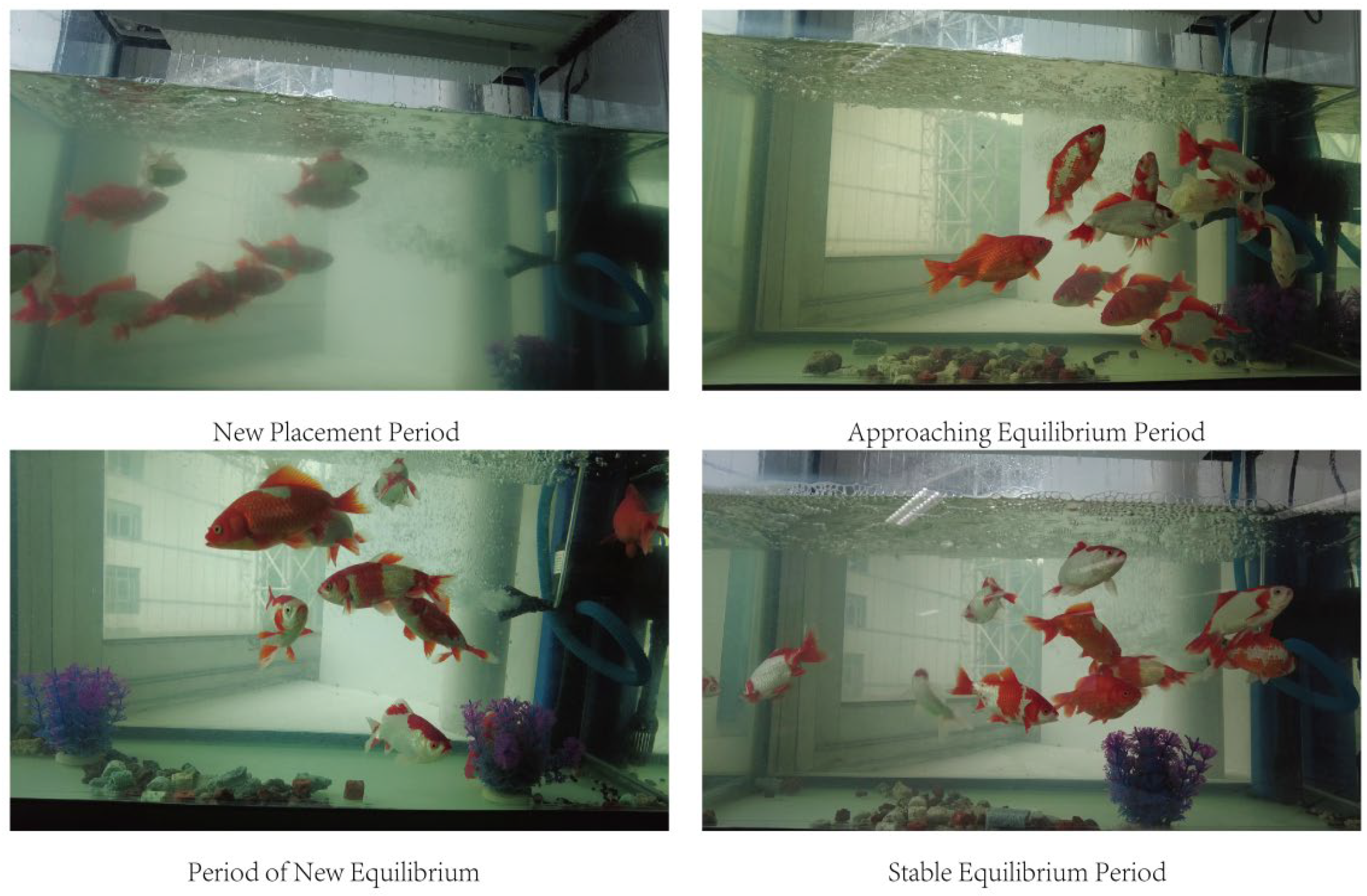
New Placement Period: At this stage, the water body and golden carp were newly added to the tank, along with the DEBAO water quality care agent, HANYANG nitrification bacteria and adsorbed substances of net hydroponic bacteria, and a water pump and oxygen changing machine were added. However, due to the failure to achieve a good balance state, the water quality was turbid. The water as a whole was green due to the growth of green algae.

(2)

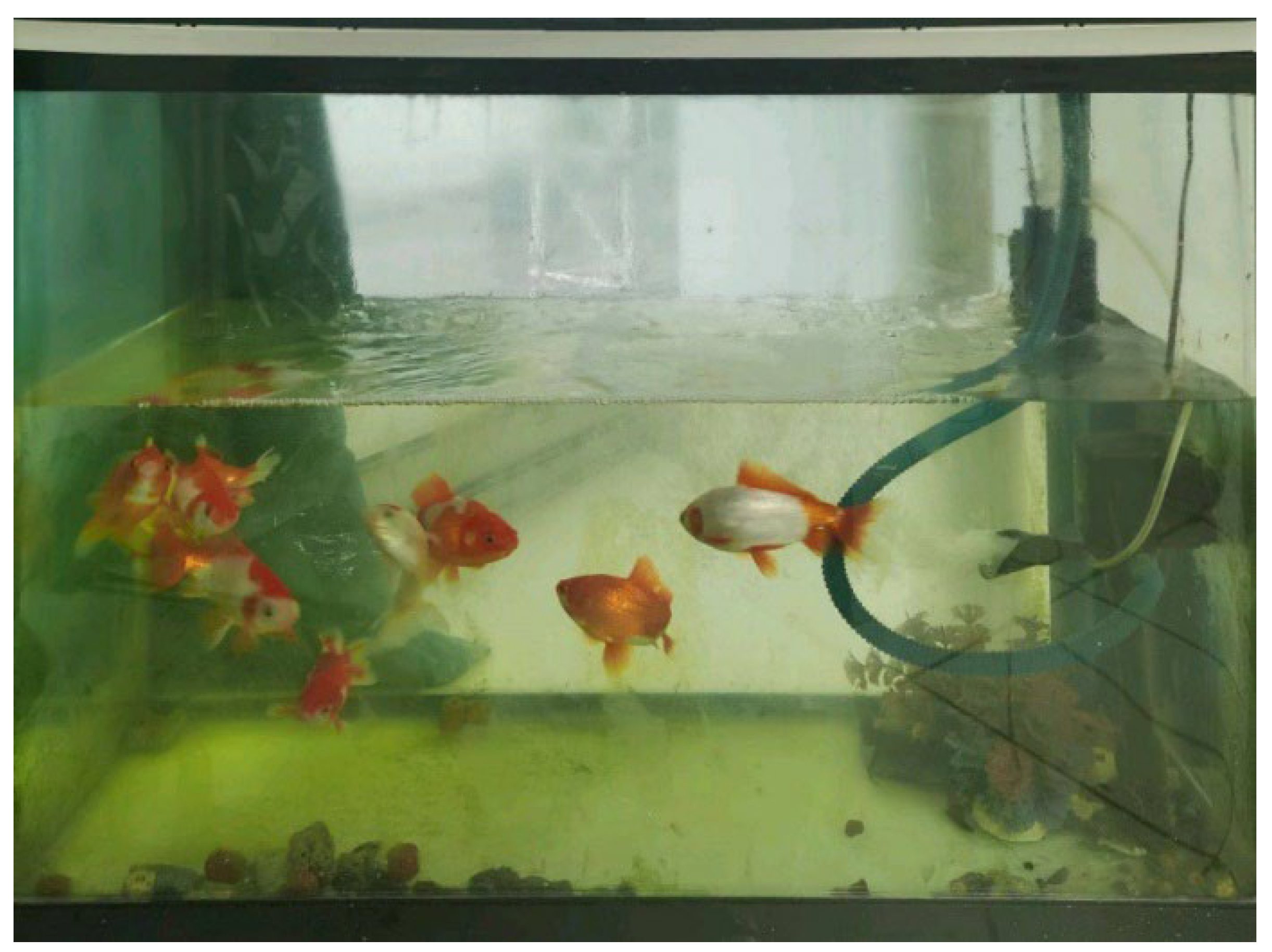
Approaching Equilibrium Period: In this stage, due to the action of nitrification bacteria, the water reached a good equilibrium state, and the overall water was relatively clear. However, because the nitrification bacteria decomposed the excreta of the golden carp into ammonia nitrogen, without adding sea salt and adsorbed substances, and with the action of some algae, the water quality was clear, and the overall water was yellowish green.

(3)

Period of New Equilibrium: In this stage, due to the appropriate addition of sea salt, EFFICIENT, IMMUNE, BACTERCIDE and other water quality care adsorbents, ammonia nitrogen was neutralized, and the water was clear. However, due to the color interference of the water quality care agents, the water body was pale blue and green.

(4)

Stable Equilibrium Period: In this stage, the water body was in equilibrium, nitrification bacteria effectively treated the excreta of the golden crucian carp, ammonia nitrogen was neutralized by sea salt, the effect of the water quality care agent disappeared, the water quality was clear and the water body was almost colorless and transparent.

The effect of the four periods is shown in Figure 3.

To ensure that our model has a stronger generalization ability, adapts to the complicated water environment and meets the detection requirements of laboratories and individual and future breeding production requests, we have a complete record of images of each phase. The new period was used to simulate the actual pond aquaculture environment. The production phase of the water quality environment was complex, with the water quality being affected by algae, turning green. Due to floating objects such as soil, the water quality was cloudy. We used the stage of trend balance and initial balance to simulate the raising environment in individual families. In this stage, the water quality was clear, and the color was relatively diverse due to different water lamps and the algae breeding environment. There were bacteria houses, small stones and other environments which fit the actual family breeding environment. The stable period was used to simulate the most ideal laboratory breeding research environment, which is suitable for laboratory research environments because the water is transparent and clear, and the water environment is simple.

2.2. Data Processing

Each second of a video (30 frames per second) contains 30 images, and we extracted all of the images per second of the video using openCV. In the adjacent frames, the golden carp moved a very limited distance. This resulted in a high degree of image similarity. If we tested directly based on this dataset, there would be a lot of redundancy, which may have led to overfitting of the model. We used the pHash algorithm to test the image similarity.

The algorithm based on mean hashing is called the average hash algorithm. This algorithm is based on comparing the average of each pixel of a grayscale map with the average of all pixel points. Although simple, AHash is very much influenced by the mean value. For example, the gamma correction or histogram equalization of an image can affect the mean value and thus the final hash value. The pHash algorithm is more robust than the AHash algorithm. pHash uses the discrete cosine transform (DCT) to obtain the low-frequency components of an image. The DCT is an image compression algorithm that transforms an image from the pixel domain to the frequency domain. In general, images have a lot of redundant and correlated information, and the DCT has good de-correlation performance. Moreover, the DCT itself is lossless, creating excellent conditions for subsequent operations in areas such as image transformation. Therefore, when pHash is used, the hash result value remains the same as long as the overall structure of the image remains the same. The effect of gamma correction or color histograms being adjusted can be avoided.

The pHash algorithm reduces the picture frequency through the DCT. Its function is to generate a “fingerprint” string for each image and then to compare the fingerprints of different images. As the results become closer, the pictures become more similar. The basic principle is as follows:

(1)

Downsize: Zoom the image down to an 8 by 8 size for a total of 64 pixels. The function of this step is to remove the details of the image, retaining only the basic information such as structure/light and shade, and to abandon the image differences caused by different sizes/proportions.

(2)

Simplify the colors: Convert the reduced image into 64 grayscale levels, i.e., all the pixel points only have 64 colors in total.

(3)

Calculate the mean: Calculate the grayscale average of all 64 pixels.

(4)

Compare the grayscale of the pixels: The gray level of each pixel is compared with the average value. If the gray level is greater than or equal to the average value, it is denoted as 1, and if the gray level is less than the average value, it is denoted as 0.

(5)

Calculate the hash value: The results of the previous comparison, combined together, form a 64-bit integer, which is the fingerprint of the image.

(6)

The order of the combination: As long as all the images are in the same order, once the fingerprint is obtained, the different images can be compared to see how many of the 64-bit bits are different. In theory, this is equivalent to the “Hamming distance” (in information theory, the Hamming distance between two strings of equal length is the number of different characters in the corresponding position of the two strings). If no more than 5 bits of data are different, the two images are similar; if more than 10 bits of data are different, this means that the two images are different.

The formula is as follows:

One-dimensional DCT transformation formula:

$$F\left(u\right)=c\left(u\right){\displaystyle \sum }_{i=0}^{N-1}f\left(i\right)cos[\frac{\left(i+0.5\right)\pi }{N}u]$$

(1)

The value of $c\left(u\right)$ is as follows:

$$c\left(u\right)=\left\{\begin{array}{c}\sqrt{\frac{1}{\mathrm{N}}},\mathrm{u}=0\\ \sqrt{\frac{2}{\mathrm{N}}},\mathrm{u}\ne 0\end{array}\right.$$

(2)

where $f\left(i\right)$ is the original signal; $F\left(u\right)$ is the coefficient after DCT transformation; N is the number of points of the original signal; and $c\left(u\right)$ is the compensation factor.

Two-dimensional DCT transformation formula:

$$F\left(u,v\right)=c\left(u\right)c\left(v\right){\displaystyle \sum }_{i=0}^{N-1}{\displaystyle \sum }_{j=0}^{N-1}f\left(i,j\right)cos[\frac{\left(i+0.5\right)\pi }{N}u]cos[\frac{\left(i+0.5\right)\pi }{N}v]$$

(3)

The value of $c\left(u\right)$ is as follows:

$$c\left(u\right)=\left\{\begin{array}{c}\sqrt{\frac{1}{N}},u=0\\ \sqrt{\frac{2}{N}},u\ne 0\end{array}\right.$$

(4)

The two-dimensional transformation is derived from the one-dimensional transformation, and the above formula can be converted to

$$\mathrm{F}={\mathrm{AfA}}^{\mathrm{T}}$$

(5)

The value of A is

$$A\left(i,j\right)=c\left(i\right)cos[\frac{\left(j+0.5\right)\pi }{N}i]$$

(6)

This form is more convenient to calculate. The DCT transformation is symmetric, so the image can be restored after DCT transformation.

We used the pHash algorithm test to select different frames of adjacent images. Through testing, within 30 1 s frames, the image similarity was higher, which could lead to a large amount of redundancy, and the model may also encounter a fitting problem. Additionally, in the subsequent image similarity comparison, when the images were spaced at 240 frames, the image similarity was already low, which could avoid the redundancy phenomenon in the model. We selected every 240 frames (every 8 s) and selected one picture to form the dataset in the experiment. In order to effectively verify the superiority of the rotating preselected box object detection algorithm, images at each stage were randomly selected as the object detection dataset, and 1160 images were labeled with the standard box and the rotating box to train the traditional object detection algorithm.

The dataset size is shown in

Table 1. Original annotated dataset size.

Annotation Type	Dataset Size
Standard box	1160
Rotating box	1160

.

Then, we cropped the datasets according to the results of the rotating object detection box. We randomly selected 3000 images of single-tailed grass carp for annotation. Due to occlusion and other reasons (other reasons are the presence of residual shadows and aggregations of fish in the captured image, which can make it impossible to label the image), we finally obtained 2912 identification datasets of 10 single-tailed golden crucian carp. Relevant data are shown in

Table 2. Size of single-fish-labeled datasets after cropping.

Dataset	Dataset Size
Standard detection datasets	500
Rotation detection datasets	2912

.

3. Materials and Methods

3.1. Detection of Golden Crucian Carp

In object detection tasks, such as SSD [30], YOLO series and face detection algorithms, such as MTCNN [31], DBFace [32] and CenterNet, all show excellent performance in different detection tasks, but the preselected box of these detection algorithms is usually a rectangular box perpendicular to the image direction. In the object detection task, when facing people, vehicles and other objects, because these targets usually do not undergo large deformation in a short time—they usually only undergo translation and rotation in the horizontal position—the rectangular box can also complete the detection task well.

In the face detection task, because the whole face can be regarded as a regular polygon, the rectangular box can sufficiently complete the detection task. However, since the movement of fish is carried out by swinging, the fish always have relevant deformation in the process of movement. However, in the traditional object detection task, large deformation does not account for a very high number of the total sample. However, fish can move freely in the three-dimensional space in the water body, which can produce large deformation in all directions. Therefore, the preselected detection box of fish cannot be sufficiently fitted to the preselected box perpendicular to the image in the process of fish movement.

In order to explore the difference between common scene detection and fish detection, face detection was taken as an example to carry out simulated detection, as shown in Figure 4. In daily life scenes, the object position in the three-dimensional space is perpendicular to the ground under the action of gravity, similar to when people stand on the ground, where the face, body and feet are perpendicular to the ground. This type of three-dimensional space is frozen in two-dimensional pictures, so almost all the objects can be a standard box. This is demonstrated in the left image in Figure 4. Even in a dense crowd, almost every face can be boxed by a single red box, and most red boxes do not have much overlap. In the right figure of Figure 4, according to the attention mechanism of the human brain, it is obvious that the fish with a white body in the middle should be the first fish to be paid attention to, so it is naturally boxed in red. Note that, at this time, the tail and fin of the fish are boxed for the integrity of the features. In addition, it is inevitable that object detection at the two-dimensional space level easily leads to an overlapping phenomenon among the fish in the image. In the process of fish movement, the area of the preselected box increases, and the possibility and area of the other fish entering the preselected box increase [33]. Therefore, the blue box can be further adapted to remove the features of the fish tail and fin, which may be irrelevant in the detection of fish objects but important in identification. Since multiple fish features may easily appear in the same box, the accuracy of identification is greatly affected. Therefore, we can take the yellow rotating box to extract a single fish to not only ensure the complete features of the fish but also to not introduce redundant features of other fish [34].

3.1.1. Rotating Box Representation

The annotation method adopted by the object detection method should be changed according to the shape characteristics of the detected object itself [35]. The application scenario of the original object detection is the object in the natural scene, and the object detection box is the horizontal bounding box (bbox). Ultimately, the perspective of the initial application scenario is the horizontal perspective. However, according to our fish identification task in the real scene, in order to better match the image features and avoid the redundant information of the network training, we need to provide a more accurate individual fish map in the object detection stage.

Through the statistics of the fish swimming posture in the real world, as shown in Figure 5, the fish posture is non-standard horizontally and vertically. Therefore, when our demand changes, the shape characteristics of the fish in the two-dimensional image change. We used the rotating object detection box for the experiment. It is beneficial to constrain the training direction of the network and to reduce the convergence time of the network.

At present, there are three common definition methods of arbitrary rotation boxes, as shown in Figure 6.

(1)

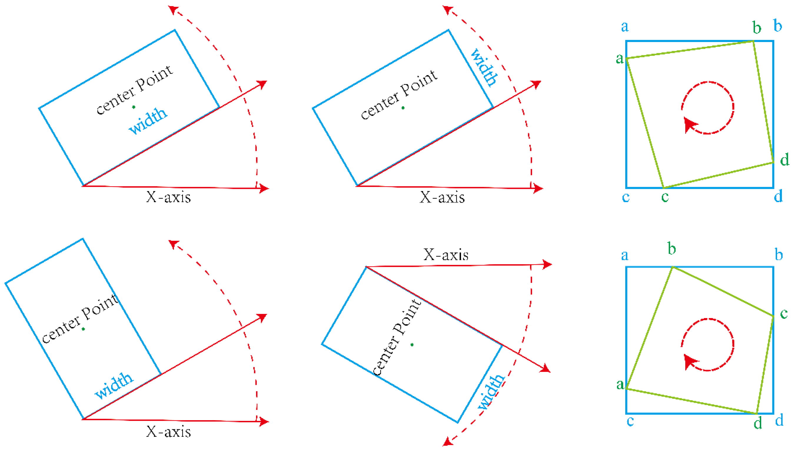
Open CV notation: The parameters are [x, y, w, h, θ], where x and y are the coordinate axes. Angle θ refers to the acute angle formed when the x-axis rotates counterclockwise and first coincides with a certain side, which is denoted as w and the other side as h. The range of θ is [−90,0).

(2)

Long side representation: The parameters are [x, y, w, h, θ], where x and y are the coordinate axes, w is the long side of the box and h is the short side of the box. Angle θ refers to the angle between the long side of the box h and the x-axis, and the range of θ is [−90,90).

(3)

Four-point notation: The parameters are [x1, y1, x2, y2, x3, y3, x4, y4]. The four-point representation does not select the coordinate axis for definition, but rather, it selects the four vertices of the quadrilateral to record the changes, starting at the leftmost point (or above if it is a standard horizontal rectangle) and sorting counterclockwise.

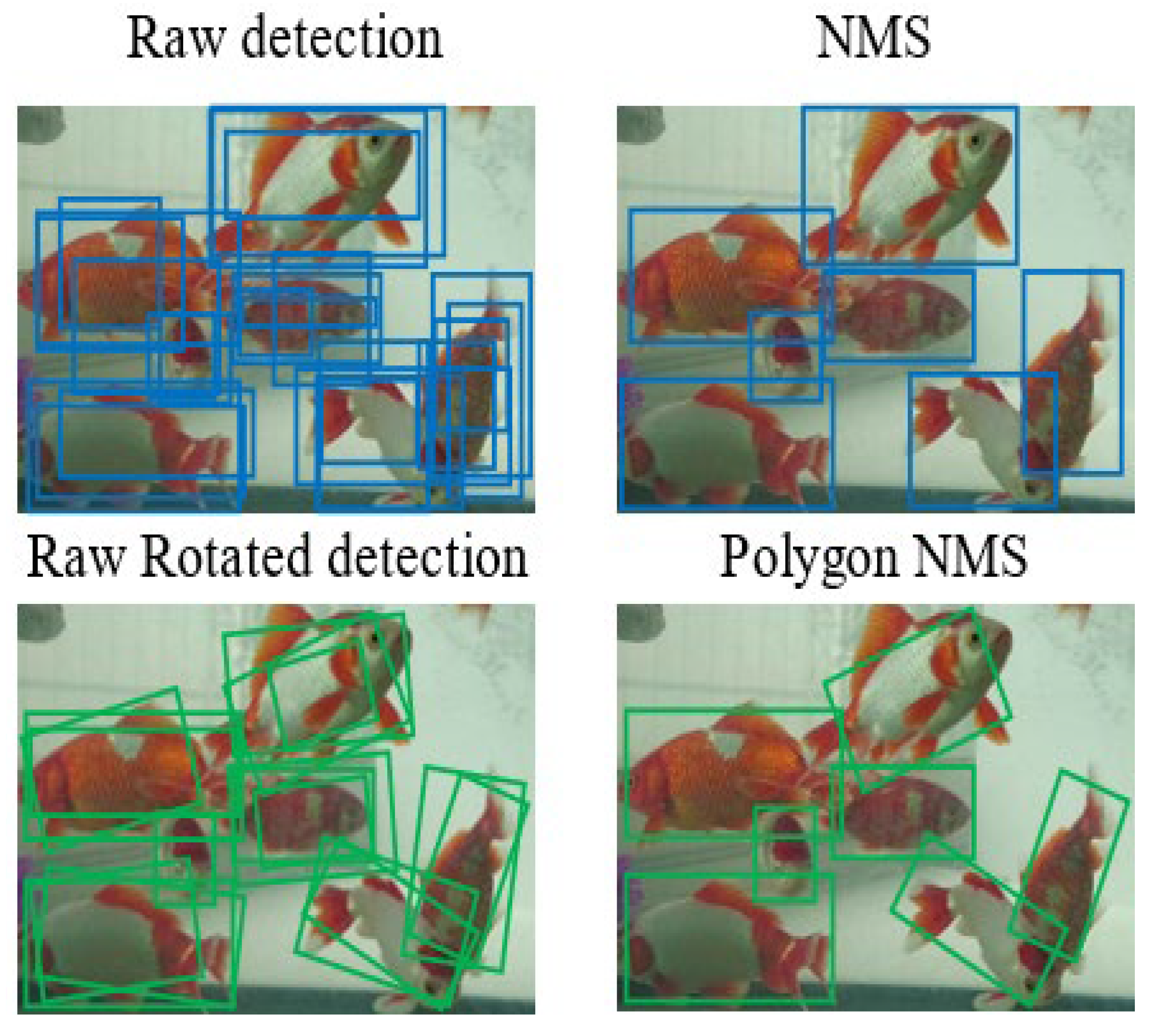
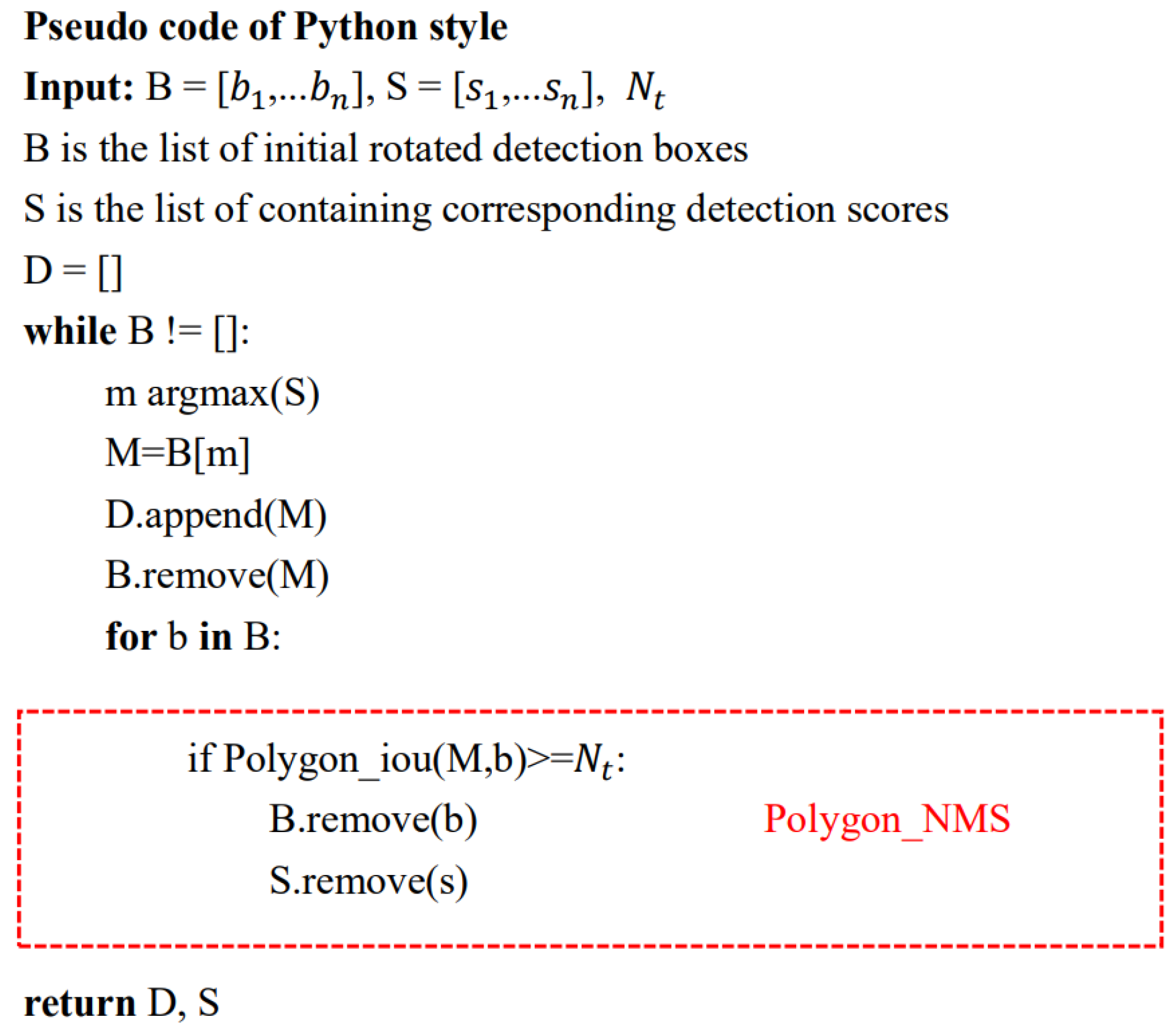
Although the rotation detection methods based on parameter regression have achieved competitive performance in different visual tasks and have become the cornerstone of many excellent detection methods, these methods are inherently subject to boundary discontinuity. In fact, all “angular based rotation box representation methods” need to predict the angle difference between the anchor and GT, but a small deviation in the angle regression results has a great impact on the final results. For the task requirements of fish identification in this paper, we do not want to introduce too many unnecessary calculations because, in essence, there are countless classes of regression prediction, and any floating-point number in [0:180] may be predicted as an angle. The change in angle is discontinuous, so it may be difficult to learn, and the learning cost is very high. This leads to a slow convergence and prediction speed of the loss function based on IoU series, which does not meet the actual needs of real-time monitoring [36].

Therefore, we approached the representation method of the rotation box from a new angle; classification was used instead of regression to achieve a better and more robust rotation detector. The root cause of the boundary problem based on the regression method is that the ideal prediction is beyond the scope of definition. A new rotation detection baseline was designed to transform the angle prediction from a regression problem into a classification problem. A circular smoothing marker (CSL) was used to address the periodicity of the angles and to increase the error tolerance between adjacent angles.

Figure 7 shows the label setting (single HOT label coding) for a standard classification problem. The conversion from regression to classification causes a certain loss of accuracy. Taking the five-parameter method for the angle range of 180° as an example, with ω (default ω = 1°) degrees for each interval as a category and without the influence of boundary conditions, a more robust angle prediction can be obtained by classification.

3.1.2. Polygon NMS

Standard NMS is generally used for standard rectangular bounding boxes (bboxes). As shown in Figure 8, the picture in the upper left corner is the raw detection of the standard bbox without NMS processing, and the one in the upper right corner is the raw detection after NMS processing. It can be seen that the NMS algorithm removes the repeated bboxes of a detected object. However, the NMS algorithm for rotating bboxes with angles has large limitations, so we adopted the Polygon NMS algorithm in the end.

Polygon NMS can remove prediction bboxes that have a high degree of coincidence but that are relatively inaccurate. The difference between Polygon NMS and NMS is that the former can handle rectangular bounding boxes at any angle, which is very suitable for our dataset.

Figure 9 is the pseudocode of Polygon NMS in Python style. It is roughly divided into the following three steps:

(1)

Sort the confidence of all predicted bboxes and obtain the one with the highest scores (add it to the list).

(2)

Solve the IoU (Polygon_IoU) in pairs with the bbox selected in the previous step, removing those boxes with an IoU greater than the threshold in the remaining bboxes.

(3)

Repeat the first two steps for all remaining boxes until the last bbox is left.

Finally, as shown in the lower right of Figure 8, after processing by the Polygon NMS algorithm, the repeated raw rotated detection was significantly reduced, which meets our needs, achieving as much as possible in extracting the characteristics of a single fish without the features of other fish.

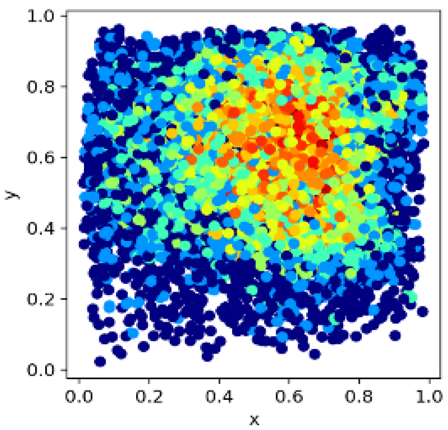
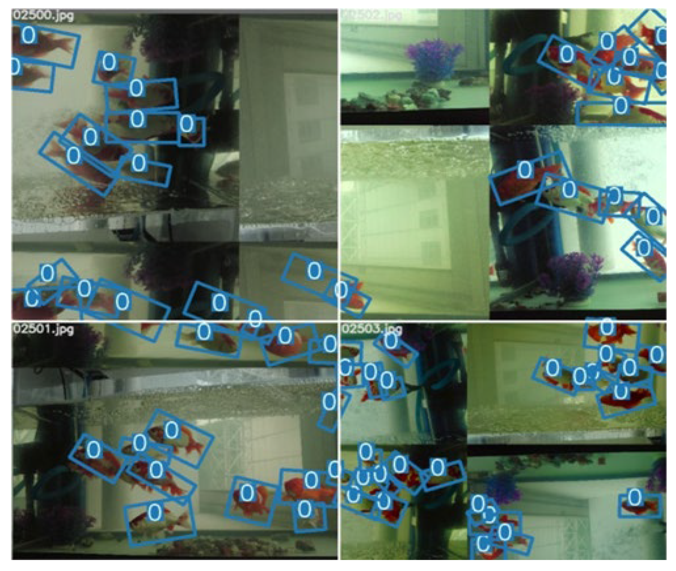
3.1.3. Handling Class Imbalance with Mosaic

Due to the particularity of the identification task, the problems in our dataset are similar to, but not the same as, those in the natural scene. Our summary is as follows:

(1)

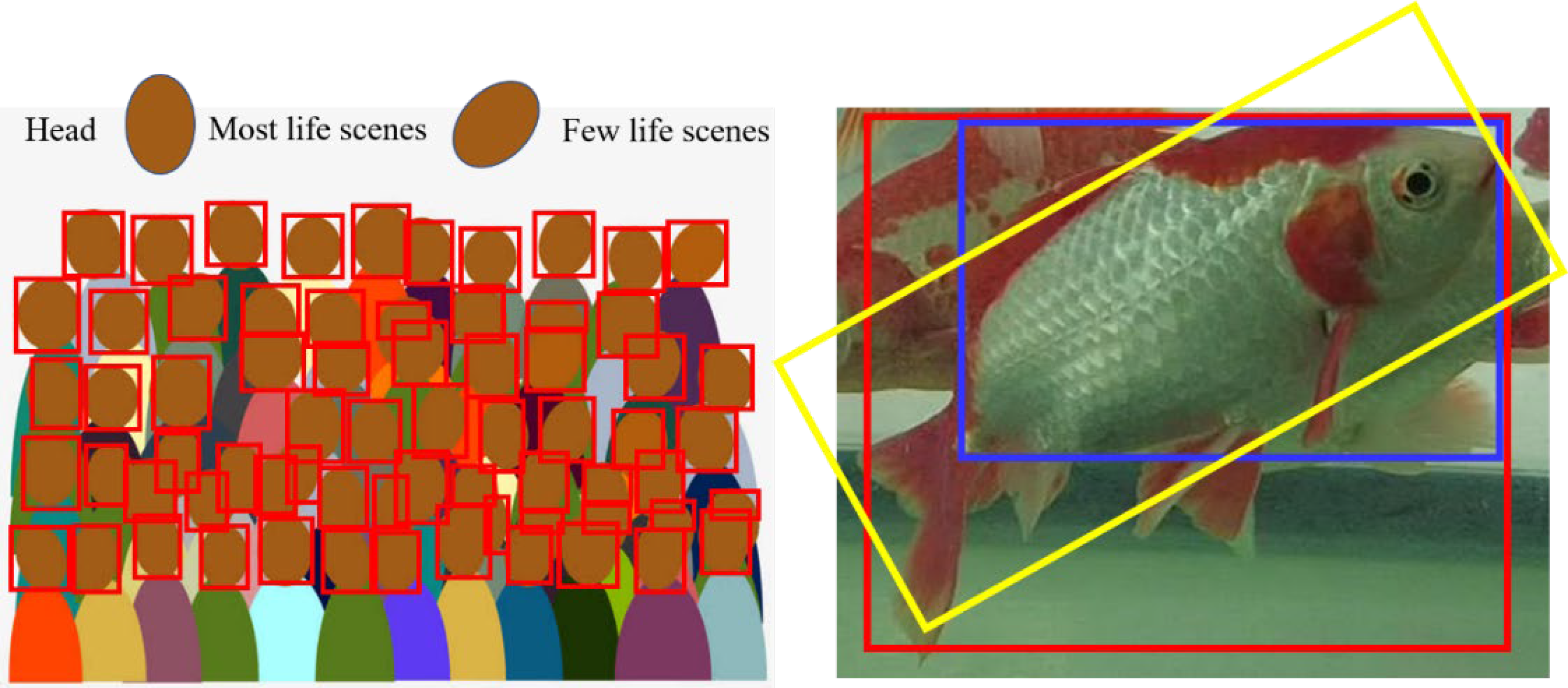
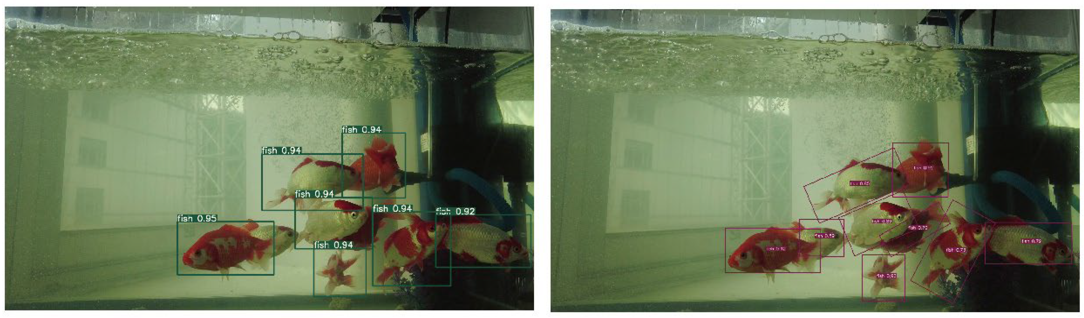
There are many targets in the fish tank, densely or sparsely arranged.

(2)

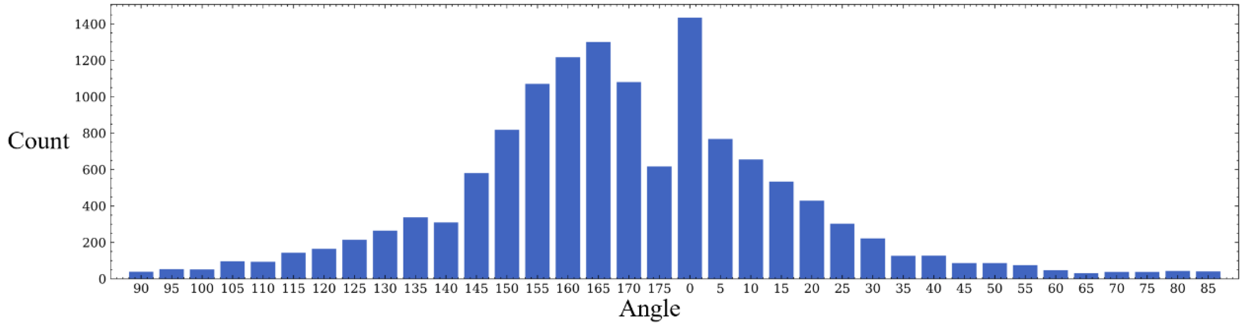
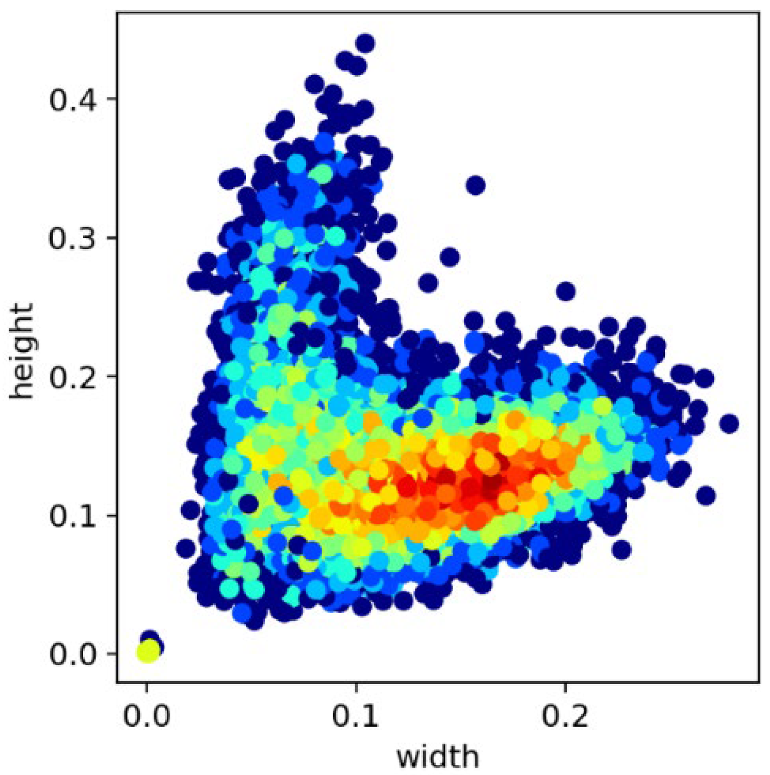
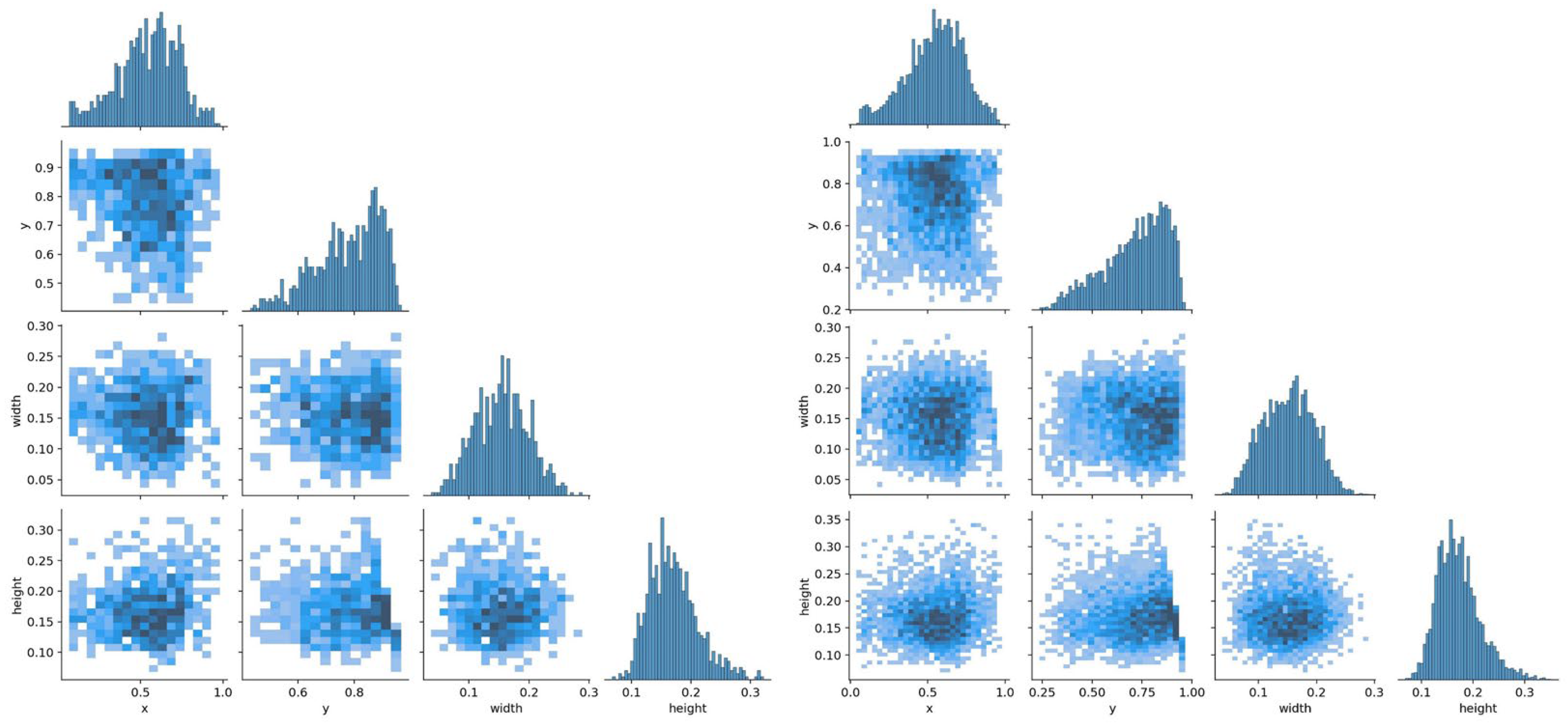
As shown in Figure 10, the position of the target object is roughly uniformly distributed. However, it can be seen in Figure 11 that, most of the time (over 90%), the fish are not swimming in the water in a completely vertical or horizontal posture, most of which have non-uniform rotation angles that are between 0 and 40 degrees and 140 and 180 degrees.

(3)

Since the image needs to be scaled, it aggravates the uneven distribution of the target object.

In order to alleviate the impact of these problems, we adopted the Mosaic strategy. Specifically, we obtained four pictures from the training dataset and then randomly selected the center point in a certain range on a large image, placing a picture in the upper left, lower left, upper right and lower right of the center point, for combined splicing. Mosaic’s splicing feature can greatly improve the uneven distribution of objects in the dataset, and due to the randomness of its splicing, as the training time increases, the improvement effect is more obvious, and to a certain extent, this operation can increase the batch size. An example is shown in Figure 12.

3.2. Identification of Golden Crucian Carp

3.2.1. Identity Recognition

Face recognition is the main application of current identity recognition, and there are no large-scale research results on the identity recognition of other animals. The essence of the face recognition operation is to transform the feature map of the face from the pixel space to another lower-dimensional space and perform similarity calculations, and then the network is trained based on the prior knowledge that the distance of the same individual’s face is always smaller than the face of different individuals. In the test phase, the embedding of the feature needs to be calculated, then the distance, and finally the threshold is used to discriminate whether the two face images belong to the same individual. Mapping the extracted feature vectors in this way such that the same individual has more accurate feature relevance is a focus area in identity recognition. Essentially, works such as ArcFace [37], SphereFace [38] and CosFace [39] all modified the existing softmax loss to achieve the goal. Due to the diversity between the human face and golden crucian carp, in order to choose a model that is more suitable for fish identification as the baseline, we selected a variety of models for the experiments. The detailed experimental results can be found in Section 4.3.

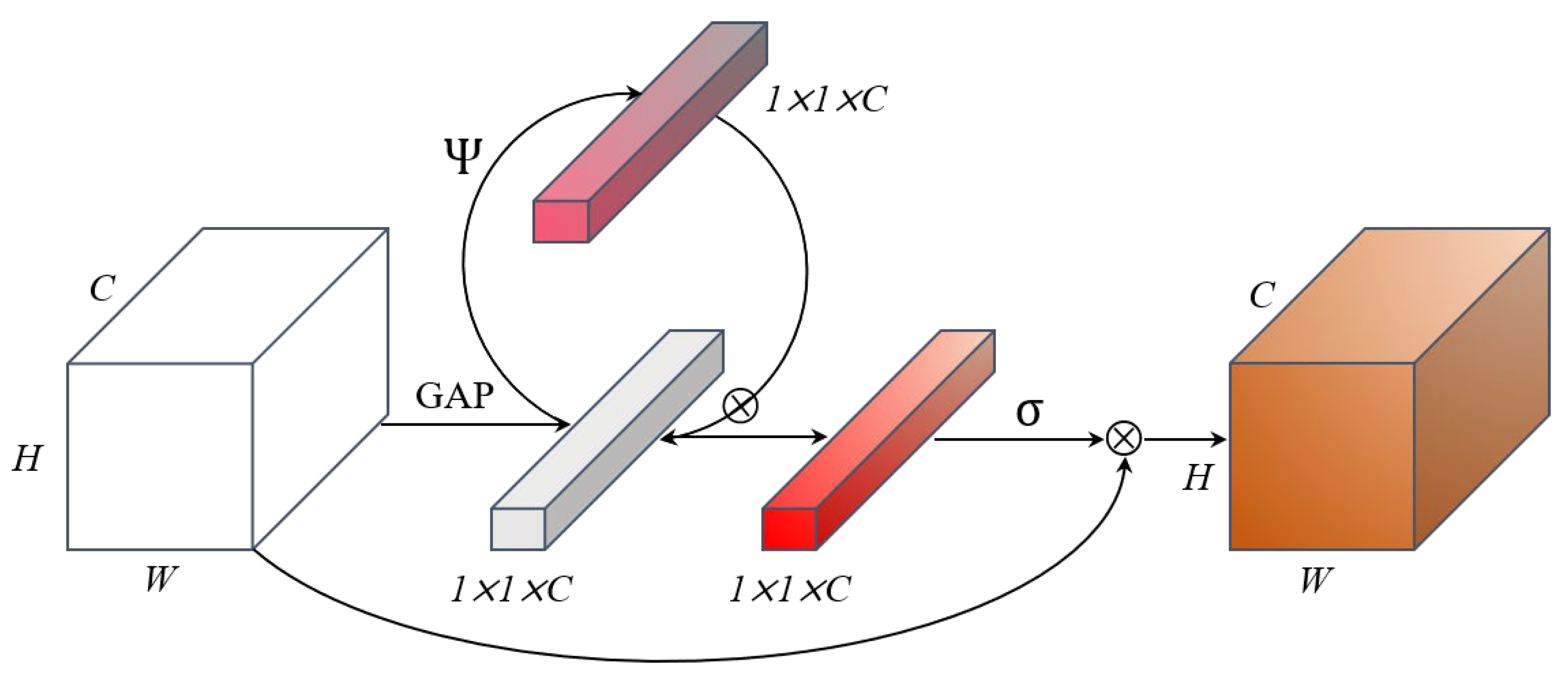
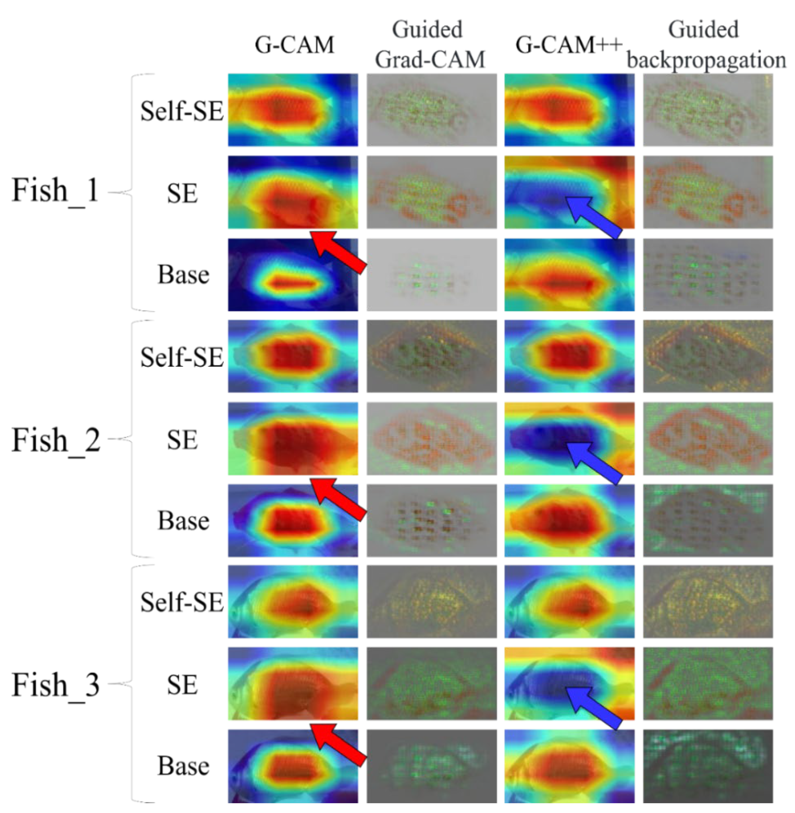
3.2.2. Self-SE Module of FFRNet

As the network deepens, the cost of the non-linear activation function decreases, because with each decrease in resolution, the memory of each convolutional layer is usually halved. Therefore, SENet introduces an attention module called the SE module, which significantly improves the accuracy without drastically delaying the inference time of the network once it is inserted into a convolutional neural network. However, in small-scale networks or datasets, this type of improvement is often restricted. In view of this, we designed a self-SE module, which aims to improve the performance of the SE module, as shown in Figure 13.

The process is based on the mapping of the input X∈RH × W × C to the output U∈RH × W × C. Next, we assumed that V = [v1, v2, vc] represents the convolution kernel and vc represents the c-th convolution kernel. Then, the conventional convolution is as follows:

$$U_c=v_c\ast X={\displaystyle \sum }_{s=1}^C{v}_c^s\ast x^s$$

(7)

Within this, ∗ represents the convolution operation. It is worth mentioning that, for the convenience of presentation, we omitted the bias term. In fact, if the batch normalization layer is used, the bias term can be omitted [40]. Similar to the SE module, the self-SE module we designed also underwent two stages of squeeze and excitation. The only difference lies in the squeeze phase, which this article focuses on.

Squeeze: Similar to the SE module, considering the signal of each channel in the output feature, each convolution kernel is equipped with a local receptive field, but this cannot make full use of the context information outside this area. To solve this problem, firstly, we adopted global average pooling (GAP) to map the output feature map X to a one-dimensional vector. Assuming that Z is the output after this squeeze operation, the c-th element of Z should be a specific value of the c-th channel after GAP. The specific calculation formula is as follows:

$$Z_c=\frac{1}{H\times W}{\displaystyle \sum }_{i=1}^H{\displaystyle \sum }_{j=1}^W{u}_c\left(i,j\right)$$

(8)

Self-Activation: In order to use the squeezed channel information, the SE module simply uses a gating mechanism with a sigmoid activation. Before this step, we inserted a self-activation mechanism with the purpose of constraining the complexity of the model and improving the model’s generalization ability, which can more fully activate the module information. Usually, a simple non-linear activation function such as a sigmoid is used. However, a sigmoid is slow in the process of derivation, so it is not the best choice. Instead, we used a piecewise activation function denoted as Ψ to simulate a sigmoid.

$$\mathsf{\Psi }\left(x\right)=\frac{ReLU\left(x+3\right)}{6}$$

(9)

$$W=F_{self-activation}\left(z\right)=\mathsf{\Psi }\left(z\right)\otimes z$$

(10)

Above, W ∈ RC denotes the output and represents the Hadamard product operation. Then, the subsequent operation is the same as the squeeze phase of the SE module. To some extent, our method is a type of dual self-correlated attention on the channel dimension, which is why it is called the self-SE module. In this paper, the network composed of the self-SE module was called FFRNet.

We selected three fish for visualization using four methods: G-CAM, G-CAM++, guided G-CAM and guided backpropagation.

G-CAM: By obtaining the weights corresponding to each pair of feature maps, a weighted sum is finally calculated. Additionally, the weights are calculated using the global average of the gradients [41].

Guided G-CAM: In this method, guided backpropagation or deconvolution is integrated into Grad-CAM, and point-wise multiplication is performed.

G-CAM++: Based on G-CAM, it adds a ReLU and weight gradient to the weight representation of the feature mapping corresponding to a certain classification [42].

Guided backpropagation: This is the classic method of model visualization [43].

Each fish datum is trained with the self-SE module, SE module and base network (excluding the SE module), and the final visualization is shown in Figure 14. It is obvious that both the self-SE module and SE module can capture the central area and outline of each target fish, whereas the performance of the base model is unsatisfactory. Furthermore, we compared the self-SE module and SE module, showing that the network with the SE module seems to extract features more efficiently than that with the self-SE module (more red areas) using the G-CAM algorithm. However, some parts of these areas are redundant, which are just part of the background of the image. As shown by the red arrow, these areas should not be the part that the network focuses on, and the SE module excessively extracts them into areas of interest. On the other hand, these background areas can be ignored while retaining the characteristics of the target object in the network with the self-SE module. In the G-CAM++ algorithm, it can be clearly seen that the self-SE module is still able to stably capture the features of the central area and effectively extract the outline of the fish. However, as indicated by the blue arrow, the network with the SE module chooses to ignore this area (because it is displayed in blue), which violates the common sense of vision. The accuracy improvement brought by the self-SE module to the network is further verified in Experiment 4.3.

4. Results

Our experiment was mainly divided into three steps.

Firstly, we verified a variety of object detection models and then chose networks with better performance as the baselines. Then, we added the rotating bounding box to the baselines for further comparison. Finally, the best rotating object detection network was used as the model in step one.

Secondly, according to the detection results of the standard bbox and the rotated bbox, we cropped the golden crucian carp image and sent it to a common identification model. The effectiveness of the rotated bbox can be proved by the recognition results.

Thirdly, we compared the results of our proposed FFRNet with those produced by a general identification model, proving the competitive strength of our method.

Through the step-by-step experiment, we can ensure that each step of our identification of golden crucian carp is a local optimal solution in order to set up an effective pipeline for the detection and identification of golden crucian carp.

4.1. Object Detection Experiment

We chose one-stage object detection networks for the purpose of ensuring that the experimental model can be deployed in mobile and embedded devices. In our experiment, mainstream models such as CenterNet, YOLOv4, YOLOv5, EfficientDet and RatinaNet [44] are used, and the best object detection model is used as the baseline. In order to comprehensively evaluate the model, we chose indicators including precision, recall, F1, mAP and inference for testing. The results predicted by the model have four cases: true positive ($TP$), false positive ($FP$), true negative ($TN$) and false negative ($FN$). The experimental results are shown in

Table 3. Different object detection models based on standard boxes, among which YOLOv5s and CenterNet have outstanding performance, outperforming the other networks in terms of speed and accuracy.

Model	P	R	F1	[email protected]	[email protected]:0.95	Inference @Batch_Size 1 (ms)
CenterNet	95.21%	92.48%	0.94	94.96%	56.38%	32
YOLOv4s	84.24%	94.42%	0.89	95.28%	52.75%	10
YOLOv5s	92.39%	95.38%	0.94	95.38%	58.31%	8
EfficientDet	88.14%	91.91%	0.90	95.19%	53.43%	128
RatinaNet	88.16%	93.21%	0.91	96.16%	57.29%	48

.

Precision (P) represents the proportion of true positives in the identified pictures:

$$Precision=\frac{TP}{TP+FP}$$

(11)

Recall (R) represents the ratio of the number of correctly identified objects to the number of all objects in the test set:

$$Recall=\frac{TP}{TP+FN}$$

(12)

F-Score is a comprehensive evaluation index of P and R. When β = 1, it is called the F1-Score.

$$F-Score=\left(1+{\beta }^2\right)\cdot \frac{ Precision \cdot Recall }{{\beta }^2\cdot Precision + Recall}$$

(13)

mAP represents the average of the area under the PR curve for all classes.

mIoU is the mean of the IoU of all predicted and true bounding boxes.

mAngle is the mean of the angles of all predicted and true bounding boxes.

Inference@batch_size 1 represents the inference time required for a picture.

In order to overcome the two problems of GPU asynchronous execution and GPU warm-up, we used virtual prediction 300 times as the GPU warm-up first and then used the code torch.cuda.synchronize() to perform synchronization between the host and the device (i.e., GPU and CPU). Therefore, time recording is only performed after the process running on the GPU is completed, overcoming the problem of asynchronous execution. Furthermore, by doing so, the real inference time of the model in the actual scene can be tested.

The experimental results show that YOLOv5 and CenterNet displayed a relatively better performance. Therefore, YOLOv5 and CenterNet were used as the baseline to improve and form a rotated bbox object detection model, R-CenterNet and R- YOLOv5, and we proceeded to the next experiment. The experimental results are shown in

Table 4. YOLOv5s and CenterNet were transformed into rotating object detection models (R-Yolov5s, R-CenterNet). In the comparison data of the two models after training, R-YOLOv5s generally scored 2–5% higher than R-CenterNet, and R-YOLOv5s was more powerful.

Model	P	R	F1	mIOU	mAngle	Inference @Batch_Size 1 (ms)
R-CenterNet	88.72%	87.43%	0.88	70.68%	8.80	76
R-YOLOv5s	90.61%	89.45%	0.90	75.15%	8.26	43

.

It can be seen that the overall performance of R- YOLOv5 was better than that of R-CenterNet, and after being modified to a rotated bounding box, the former could still guarantee a relatively high speed. Unfortunately, the accuracy of the model was still far from that required for the actual deployment application, so we used a variety of training tricks to optimize the model performance and further conducted ablation experiments to extract the best model training configuration.

HSV_Aug: The variation range of the hue, saturation and brightness of the image HSV is (−0.015, +0.015), (−0.7, +0.7) and (−0.4, +0.4), respectively.

FocalLoss: We used FocalLoss to suppress the background class and imitate the method of retinanet, setting the class weight α to 0.25 and the difficult sample adjustment parameter γ to 2.

Mosaic: Data augmentation techniques such as Mosaic and MixUp were used. See Section 3.1 for details.

MixUp: See Section 3.1 for details.

Fliplrud: Flipping up, down, left and right with a probability of 0.5.

RandomScale: Random scale modification technique scaling the training image to 0.5–1.5 times the size of the original image.

As shown in

Table 5. Ablation experiments were performed on R-YOLOv5s, each time using a different training strategy. Using each strategy has an impact on the model, but it is worth noting that the addition of FocalLoss makes the model performance worse.

HSV_Aug	FocalLoss	Mosaic	MixUp	Fliplrud	Other Tricks	[email protected]
						77.32%
√						77.98%
√	√					77.42%
√	√	√				79.05%
√	√	√	√			81.12%
√			√			81.64%
√	√	√		√		80.68%
√	√			√	Fliplrud	81.37%
√		√	√	√	Fliplrud	82.46%
√				√	Fliplrud RandomScale	79.99%
√	√	√	√	√	Fliplrud RandomScale	82.88%

, we further studied the impact of different training tricks on network accuracy. We considered that the addition of each training technique has a certain impact on the accuracy of the network, but some techniques cannot improve the accuracy of the network. Although FocalLoss is often used in unbalanced data and to suppress the background class in object detection, the accuracy of the model processed by FocalLoss decreased under the dataset and corresponding settings in this paper. We speculated that the reason may be that the space allocation between the background and the object class in the data was not obviously out of balance, which led to FocalLoss not working. As shown in Figure 10, the range of the motion of fish almost covers all the positions in the image. According to our statistics, the ratio of the area of the fish’s bbox to the background in the data is about 1:2, likely making FocalLoss useless. All of our detectors use pre-trained weights, and the result shows that tricks other than FocalLoss are critical for the detectors. We observed that, due to various improvements, R-YOLOv5 demonstrated strong detection capabilities, with the highest mAP reaching 82.88%, which can be deployed in the actual external environment.

4.2. Verification of the Rotated Bounding Box

We chose Pytorch as the backend of the model and conducted related tests on RTX3060. The size of the image in the dataset was set to 112 × 112 to ensure that the model had a high running speed. We chose the SGD optimizer with an initial learning rate of 0.01. The momentum and weight decay were, respectively, set to 0.9 and 0.0005. We set nesterov to True. We used the first 1/25 epochs for the warm-up and adjusted the learning rate for each training stage after the warm-up. When the epoch equals 100, 150 and 180, the total epoch is 200. We cropped the standard and rotated bboxes of the output results of the object detection to construct a dataset with each image in it containing only a single fish, and then the new dataset was used for identification. Since ten independent individuals of golden crucian carp were selected as experimental objects, theoretically, after object detection, each image with global elements should produce ten fish samples. If we select 500 samples containing only a single golden carp for identification training, then only 50 global images are needed for object detection processing. However, due to the existence of occlusion and other factors, it is difficult for an image to contain all individual fish. Therefore, we selected 100 global images for object detection instead. In the end, the standard object detection model obtained 873 golden crucian carp individuals, and the rotated object detection model obtained 969 golden crucian carp individuals. When labeling data, we found that the rotated object detection can effectively avoid multiple golden crucian carp being detected only as a single fish caused by mutual occlusions or the overlap of fish. In identity labeling, it is difficult to label correctly if the features of multiple fish appear in a picture. When the data can be obtained effectively, after 100 pictures are extracted, they can be used as a dataset for subsequent identification experiments, and the rotated object detection model can increase the identification data acquisition rate by 9.6%. For further verification, we randomly selected 500 pictures from the two identification validation sets for the identification experiments. The result is shown in Figure 15.

When verifying the identification results, in order to effectively test the results of the detection bbox, we chose mainstream identification models, including softmax, FaceNet, ArcFace, CosFace and SphereFace. The results are shown in

Table 6. Comparative experiment of traditional identification network. The data are divided into two parts: one part is the rotated and cropped picture, and the other part is the data of the standard box. The two parts of the data are the same. The purpose is to show whether the rotating object detection has an advantage, and the result obviously shows that the performance of the model in the rotation detection column exceeds most of the other columns.

Model_Head	Backbone	Rotated Detection 500		Standard Detection 500
		Acc@Top1	Acc@Top5	Acc@Top1	Acc@Top5
Softmax	ResNet50	84.17	96.46	83.83	96.11
FaceNet	ResNet50	86.32	98.13	80.01	94.87
	ResNet101	86.18	98.43	82.36	96.08
	ResNet152	81.81	95.04	80.76	95.01
ArcFace	ResNet50	64.69	94.69	62.19	90.31
	ResNet101	69.06	92.81	65.94	92.5
	ResNet152	64.38	93.44	64.69	92.5
CosFace	ResNet50	64.06	92.81	62.19	87.81
	ResNet101	63.75	90.94	65.94	87.81
	ResNet152	65.31	86.56	59.38	85.62
SphereFace	ResNet50	62.19	89.06	50.31	85.31
	ResNet101	62.19	90.0	59.69	87.81
	ResNet152	59.69	85.62	57.81	82.19

.

The experimental results show that, compared with the traditional object detection model, the identity recognition model can achieve better recognition results on the dataset produced by the rotated object detection model. From this, we can see that rotated object detection can more effectively adhere to the outline of golden crucian carp and reduce the area of useless features, preventing other golden crucian carp from appearing in the detection bbox, which interferes with identity recognition.

By comparing YOLOv5 and R-YOLOv5, we found that the rotated object detection model had a better identification acquisition rate, and the effectively acquired identification dataset also had a higher quality when applied to the identification model.

4.3. FFRNet

In the previous section, we proved that the rotated bounding box dataset was better than the standard one, which motivated us to expand the dataset. The following experiment took 2912 pictures, with no difference in the data label format of each one, from the rotated bounding box dataset. As shown in Figure 16, the data distribution was roughly the same and roughly obeys the normal distribution.

After the dataset was expanded, we used the model above to conduct further experiments. The results are shown in

Table 7. Comparative experiment of traditional identification network. The data are a picture after being rotated and cropped. FaceNet achieved the best performance among the different backbones.

Model_Head	Backbone	Rotated Detection 2912
		Acc@Top1	Acc@Top5
Softmax	ResNet50	85.78	96.45
FaceNet	ResNet101	86.19	96.78
	ResNet50	85.02	96.34
	ResNet101	87.89	97.08
ArcFace	ResNet152	89.13	99.13
	ResNet50	80.86	91.88
	ResNet101	81.02	94.8
CosFace	ResNet152	82.22	94.53
	ResNet50	81.68	91.33
	ResNet101	79.26	91.95
SphereFace	ResNet152	80.47	92.88
	ResNet50	81.68	91.33
	ResNet101	79.96	90.7
	ResNet152	80.94	91.31

.

We also set up an identification network experiment. The training process was the same as that for the rotated object detection. From the experimental results, it can be seen that FaceNet was more suitable for this task when dealing with golden crucian carp identification. Therefore, we used FaceNet as the baseline for comparison. In addition, we further added the self-SE module to propose a network, FFRNet (fish face recognition network), which is more robust for this task and which was compared to a range of recent state-of-the-art approaches with different backbones, including MobileNetV1, MobileNetV2, MobileNetV3, ShuffleNetV2 [45], RegNet [46], InceptionV3 [47] and ResNet used by FFRNet. The results of the comparative experiment are shown in

Table 8. Comparative experiment of different models and FFRNet. In addition to the real-time inference speed, FFRNet achieved the best results. The picture size of the experimental table is 64×64.

Backbone	Image_Shape = (112,112,3) BatchSize = 64
	Accuracy	Precision	Recall	F1	Inference Time (ms)
MobileNetv1	85.2	85.22	86.17	85.69	2.916
MobileNetv2	87.51	87.68	87.53	87.54	5.237
MobileNetv3_Small	86.22	86.17	86.15	86.1	4.870
MobileNetv3_Large	88.15	88.22	88.14	88.1	6.242
ShuffleNetv2	87.45	87.48	87.5	87.38	7.243
RegNet_400 MF	87.68	87.68	87.79	87.67	14.876
inception_resnetv1	86.48	86.7	86.64	86.54	21.512
ResNet50	87.3	87.5	87.35	87.24	12.72
FFRNet	90.13	89.98	89.76	89.87	4.782

.

For the dataset with each image in it having a size of 112 × 112, FFRNet displayed the most outstanding performance. In order to further illustrate the superiority of our model, we additionally used a dataset with each image in it having a size of 224 × 224 to conduct experiments. We also added EfficientNet and the Vision Transformer [48] as experimental comparison models. The experimental results are shown in

Table 9. Comparative experiment of different models and FFRNet. In addition to the real-time inference speed, FFRNet achieved the best results. Although FFRNet (5.720 ms) was slower than MobileNetv1 (5.306 ms), after weighing accuracy, we think it is acceptable to lose a little bit of speed to guarantee extremely high accuracy.

Backbone	Image_Shape = (224,224,3)
	Accuracy	Precision	Recall	F1	Inference Time (ms)
MobileNetv1	85.92	86.05	85.99	86.01	5.306
MobileNetv2	88.2	88.32	88.26	88.18	10.332
MobileNetv3_Small	87.92	88.06	87.91	87.86	6.656
MobileNetv3_Large	88.84	88.82	88.77	88.73	11.962
ShuffleNetv2	89.0	89.05	89.01	88.92	8.224
RegNet_400 MF	89.5	89.51	89.52	89.45	22.302
EfficientNetv1_B0	89.85	89.94	89.92	89.82	16.906
inception_resnetv1	87.03	87.14	87.09	87.01	34.905
ResNet50	89.75	89.71	89.68	89.63	11.081
vision_transformer	84.63	84.85	84.69	84.67	26.768
FFRNet	92.01	91.87	91.66	91.76	5.720

.

5. Discussion

5.1. Contribution to Fish Facial Recognition

In recent years, with the strong rise of artificial intelligence, the use of computer vision models in the fishing industry has gradually become increasingly popular. One such application is fish face recognition, which can make fish farming and management more efficient and convenient. The difference between fish face recognition and human face recognition is that the features of fish faces are more subtle and smaller objects than those of human faces. Therefore, models for face recognition face difficulties in fish face recognition. Additionally, unlike human faces, fish have a large degree of overlap in space, so it is easy to introduce redundant features that affect the accuracy of identity recognition. In this paper, the data were annotated by rotating the box to avoid the impact of a large amount of redundant information on fish identity recognition. Moreover, this paper proposes a self-SE module that is more conducive to feature extraction, which was implanted in FaceNet to obtain FFRNet. Compared with other methods, our model has a great advantage in terms of speed and accuracy, and the model achieved an accuracy of over 90% in relation to satisfying real-time detection. The method provides ideas for the practical application of fish face recognition and will be considered for deployment in real environments in the future.

5.2. Robustness of the Process

Our work is an exploratory trial aimed at exploring whether face recognition can be transferred to fish facial recognition. Nonetheless, we simulated real-life situations to facilitate future practical deployment in fisheries. We chose to use a large breeding tank to simulate the real environment. We added nitrifying bacteria to the transparent tanks, which break down the fish excrement into ammonia nitrogen to simulate the real environment as closely as possible. Additionally, with the algae, the overall water had a yellowish green color. This water quality poses a challenge to our model. The real underwater environment is unlit, but the top is translucent. We simulated this realistic lighting in the tank, which is suitable for sampling the right images while simulating the underwater environment as closely as possible.

5.3. Comparison of This Method with Other Methods

Currently, most identification methods in the fish farming industry use radio frequency identification (RFID) technology. This method has high identification accuracy and a low technical threshold, but high equipment and manpower costs. In contrast to other identification models, the remaining models use a standard box for object detection and then recognize the features within the box. However, this ignores the interference caused by the pose of the fish. The two-stage model for golden carp based on rotating box object detection and identity recognition proposed in this paper not only guarantees more than 90% recognition accuracy but also has minimal equipment and manpower costs. In the future, farming technology combined with artificial intelligence technology will become a new paradigm in the farming industry.

5.3.1. Standard and Rotating Boxes

We counted fish poses in real-life scenes and found that the fish usually appeared tilted, making it difficult to achieve a perfect fit to the fish with a standard box and tending to introduce redundant features within the box. We therefore chose to use rotating boxes to solve this problem. For the training process of rotating boxes, we transformed the predicted angle from a regression problem into a classification problem and used a circular smoothing label to solve the problem of the unstable convergence of the angle loss function, which is prone to sudden changes.

5.3.2. Feature Extractor

In this article, we replaced FaceNet’s backbone and tested multiple lightweight backbones.

For example, MobileNetv1 uses depth separable convolution, which greatly reduces the number of parameters and improves the operation speed. MobileNetv2 increases the residual structure and linear bottlenecks. MobileNetv3 redesigns the network layer structure to use the h-swish activation function. However, the biggest problem of the MobileNet series is that the memory access cost of deep separable convolution is high, and the deployment speed is fast on CPU devices. However, the speed is slow for GPU. GhostNet discovers the problem of feature map redundancy and reactivates the feature layer with a linear map. These networks all have one thing in common; they reduce the number of redundant features and parameters as much as possible while ensuring accuracy [49]. Therefore, this paper draws on this idea and proposes a self-SE structure. Compared with the SE structure, we inserted a self-activation mechanism to constrain the complexity of the model, screened the channels to be activated again, reduced the honor features as much as possible and improved the generalization ability of the model. We inserted the self-SE module into FaceNet to obtain FFRNet for identity identification. We conducted a comparative experiment between FFRNet and the current mainstream lightweight networks. It is reported in Table 8 and Table 9 that the accuracy of FFRNet was higher than that of the other models, reaching 92.01%.

6. Conclusions

We effectively detected golden crucian carp through the method of rotated object detection and then carried out image cropping to avoid the problem where the traditional object detection cannot effectively capture the target fish, which causes a large, invalid and redundant area. Subsequently, we modified the relevant model of face recognition and proposed our model called FFRNet, which is the first to apply identity recognition to fish research. With a two-step pipeline that detects first and then recognizes, our model guarantees an accuracy of about 90%. Moreover, the model guarantees an operation speed of 200 FPS on a personal computer, which can effectively meet the relevant requirements of real-time detection.

In the future, our research will be further developed from the following aspects:

In terms of research goals, we will choose the grass carp, which is the most widely cultivated freshwater fish in China and can achieve extremely high economic value, as the research content. Since the characteristics of grass carp are far less obvious than those of golden crucian carp, we will consider adding some hardware to the traditional pure computer vision method, such as more refined data sampling through a one-way flow pipeline, which may solve the problem of the insufficient features of grass carp.

In terms of function, on the basis of completing the research on identity recognition, we will add more computer vision tasks, such as pose estimation, fish disease semantic segmentation and behavior prediction to form a systematic golden carp detection system. This will meet the requirements of the real-time detection of fish and realize all-round detection of farms in the future.

In terms of the environment, the current environment is relatively simple. Although it can match the environment of ornamental fish and experimental breeding tanks, it is still too simple for the actual breeding environment. Therefore, we considered ways to increase the complexity of the environment, such as increasing the turbidity and the amount of underwater debris, to enhance the robustness of the model.

References

1. Zhao, H.F.; Feng, L.; Jiang, W.D.; Liu, Y.; Jiang, J.; Wu, P.; Zhao, J.; Kuang, S.Y.; Tang, L.; Tang, W.N.; et al. Flesh Shear Force, Cooking Loss, Muscle Antioxidant Status and Relative Expression of Signaling Molecules (Nrf2, Keap1, TOR, and CK2) and Their Target Genes in Young Grass Carp (Ctenopharyngodon idella) Muscle Fed with Graded Levels of Choline. PLoS ONE 2015, 10, e0142915. [Google Scholar] [CrossRef] [PubMed]
2. Obasohan, E.E.; Agbonlahor, D.E.; Obano, E.E. Water pollution: A review of microbial quality and health concerns of water, sediment and fish in the aquatic ecosystem. Afr. J. Biotechnol. 2010, 9, 423–427. [Google Scholar]
3. Zhang, G.; Tao, S.; Lina, Y.U.; Chu, Q.; Jia, J.; Gao, W. Pig Body Temperature and Drinking Water Monitoring System Based on Implantable RFID Temperature Chip. Trans. Chin. Soc. Agric. Mach. 2019, 50, 297–304. [Google Scholar]
4. Blemel, H.; Bennett, A.; Hughes, S.; Wienhold, K.; Flanigan, T.; Lutcavage, M.; Lam, C.H.; Tam, C. Improved Fish Tagging Technology: Field Test Results and Analysis. In Proceedings of the OCEANS 2019—Marseille, IEEE, Marseille, France, 17–20 June 2019. [Google Scholar]
5. Sun, Z.J.; Xue, L.; Yang-Ming, X.U.; Wang, Z. Overview of deep learning. Appl. Res. Comput. 2012, 29, 2806–2810. [Google Scholar]
6. He, K.; Zhang, X.; Ren, S.; Sun, J. Deep Residual Learning for Image Recognition. In Proceedings of the 2016 IEEE Conference on Computer Vision and Pattern Recognition (CVPR), Las Vegas, NV, USA, 27–30 June 2016. [Google Scholar]
7. Long, J.; Shelhamer, E.; Darrell, T. Fully Convolutional Networks for Semantic Segmentation. IEEE Trans. Pattern Anal. Mach. Intell. 2015, 39, 640–651. [Google Scholar]
8. Howard, A.G.; Zhu, M.; Chen, B.; Kalenichenko, D.; Wang, W.J.; Weyand, T.; Andreetto, M.; Adam, H. MobileNets: Efficient Convolutional Neural Networks for Mobile Vision Applications. arXiv 2017, arXiv:1704.04861. [Google Scholar]
9. Sandler, M.; Howard, A.; Zhu, M.; Zhmoginov, A.; Chen, L.C. MobileNetV2: Inverted Residuals and Linear Bottlenecks. In Proceedings of the 2018 IEEE/CVF Conference on Computer Vision and Pattern Recognition (CVPR), Salt Lake City, UT, USA, 18–23 June 2018. [Google Scholar]
10. Howard, A.; Sandler, M.; Chen, B.; Wang, W.J.; Chen, L.C.; Tan, M.X.; Chu, G.; Vasudevan, V.; Zhu, Y.K.; Pang, R.; et al. Searching for MobileNetV3. In Proceedings of the 2019 IEEE/CVF International Conference on Computer Vision (ICCV), Seoul, Korea, 27 October–2 November 2020. [Google Scholar]
11. Han, K.; Wang, Y.; Tian, Q.; Guo, J.Y.; Xu, C.J.; Xu, C. GhostNet: More Features from Cheap Operations. In Proceedings of the 2020 IEEE/CVF Conference on Computer Vision and Pattern Recognition (CVPR), Seattle, WA, USA, 13–19 June 2020. [Google Scholar]
12. Tan, M.; Chen, B.; Pang, R.; Vasudevan, V.; Sandler, M.; Howard, A.; Le, Q. MnasNet: Platform-Aware Neural Architecture Search for Mobile. In Proceedings of the 2019 IEEE/CVF Conference on Computer Vision and Pattern Recognition (CVPR), Long Beach, CA, USA, 15–20 June 2018. [Google Scholar]
13. Redmon, J.; Divvala, S.; Girshick, R.; Farhadi, A. You Only Look Once: Unified, Real-Time Object Detection. In Proceedings of the 2016 IEEE Conference on Computer Vision and Pattern Recognition (CVPR), Las Vegas, NV, USA, 27–30 June 2016. [Google Scholar]
14. Redmon, J.; Farhadi, A. YOLO9000: Better, Faster, Stronger. In Proceedings of the IEEE Conference on Computer Vision & Pattern Recognition, Honolulu, HI, USA, 21–27 July 2017; pp. 6517–6525. [Google Scholar]
15. Redmon, J.; Farhadi, A. YOLOv3: An Incremental Improvement. arXiv 2018, arXiv:1804.02767. [Google Scholar]
16. Bochkovskiy, A.; Wang, C.Y.; Liao, H. YOLOv4: Optimal Speed and Accuracy of Object Detection. arXiv 2020, arXiv:2004.10934. [Google Scholar]
17. Zhou, X.; Wang, D.; Krhenbühl, P. Objects as Points. arXiv 2019, arXiv:1904.07850. [Google Scholar]
18. Tan, M.; Pang, R.; Le, Q.V. EfficientDet: Scalable and Efficient Object Detection. In Proceedings of the 2020 IEEE/CVF Conference on Computer Vision and Pattern Recognition (CVPR), Seattle, WA, USA, 13–19 June 2020. [Google Scholar]
19. Jiang, Y.; Zhu, X.; Wang, X.; Yang, S.; Li, W.; Wang, H.; Fu, P.; Luo, Z. R2CNN: Rotational region CNN for orientation robust scene text detection. arXiv 2017, arXiv:1706.09579. [Google Scholar]
20. Ding, J.; Xue, N.; Long, Y.; Xia, G.S.; Lu, Q. Learning RoI Transformer for Oriented Object Detection in Aerial Images. In Proceedings of the 2019 IEEE/CVF Conference on Computer Vision and Pattern Recognition (CVPR), Long Beach, CA, USA, 15–20 June 2019. [Google Scholar]
21. Chen, P.; Swarup, P.; Matkowski, W.M.; Kong, A.W.K.; Han, S.; Zhang, Z.; Rong, H. A study on giant panda recognition based on images of a large proportion of captive pandas. Ecol. Evol. 2020, 10, 3561–3573. [Google Scholar] [CrossRef]
22. Hansen, M.F.; Smith, M.L.; Smith, L.N.; Salter, M.G.; Baxter, E.M.; Farish, M.; Grieve, B. Towards on-farm pig face recognition using convolutional neural networks. Comput. Ind. 2018, 98, 145–152. [Google Scholar] [CrossRef]
23. Parkhi, O.M.; Vedaldi, A.; Zisserman, A. Deep face recognition. In Proceedings of the British Machine Vision Conference (BMVC), Swansea, UK, 7–10 September 2015; Volume 1, pp. 41.1–41.12. [Google Scholar]
24. Freytag, A.; Rodner, E.; Simon, M.; Loos, A.; Kühl, H.S.; Denzler, J. Chimpanzee Faces in the Wild: Log-Euclidean CNNs for Predicting Identities and Attributes of Primates. In German Conference on Pattern Recognition; Springer International Publishing: Cham, Switzerland, 2016. [Google Scholar]
25. Crouse, D.; Jacobs, R.L.; Richardson, Z.; Klum, S.; Jain, A.; Baden, A.L.; Tecot, S.R. LemurFaceID: A face recognition system to facilitate individual identification of lemurs. BMC Zool. 2017, 2, 2. [Google Scholar] [CrossRef]
26. Salman, A.; Jalal, A.; Shafait, F.; Mian, A.; Shortis, M.; Seager, J.; Harvey, E. Fish species classification in unconstrained underwater environments based on deep learning. Limnol. Oceanogr. Methods 2016, 14, 570–585. [Google Scholar] [CrossRef]
27. Chen, G.; Peng, S.; Yi, S. Automatic Fish Classification System Using Deep Learning. In Proceedings of the 2017 IEEE 29th International Conference on Tools with Artificial Intelligence (ICTAI), Boston, MA, USA, 6–8 November 2017. [Google Scholar]
28. Funkuralshdaifat, N.F.; Talib, A.Z.; Osman, M.A. Improved deep learning framework for fish segmentation in underwater videos. Ecol. Inform. 2020, 59, 101121. [Google Scholar]
29. Schroff, F.; Kalenichenko, D.; Philbin, J. FaceNet: A Unified Embedding for Face Recognition and Clustering. In Proceedings of the IEEE Conference on Computer Vision and Pattern Recognition (CVPR), Boston, MA, USA, 7–12 June 2015. [Google Scholar]
30. Liu, W.; Anguelov, D.; Erhan, D.; Szegedy, C.; Reed, S.; Fu, C.Y.; Berg, A.C. SSD: Single Shot MultiBox Detector. In Proceedings of the European Conference on Computer Vision, Amsterdam, The Netherlands, 8–16 October 2016; Springer: Cham, Switzerland, 2016. [Google Scholar]
31. Zhang, K.; Zhang, Z.; Li, Z.; Qiao, Y. Joint Face Detection and Alignment Using Multitask Cascaded Convolutional Networks. IEEE Signal Process. Lett. 2016, 23, 1499–1503. [Google Scholar] [CrossRef]
32. GitHub Repository. Available online: https://github.com/dlunion/DBFace (accessed on 21 March 2020).
33. Lauer, J.; Zhou, M.; Ye, S.; Menegas, W.; Schneider, S.; Nath, T.; Rahman, M.M.; Santo, V.D.; Soberanes, D.; Feng, G.; et al. Multi-animal pose estimation, identification and tracking with DeepLabCut. Nat. Methods 2022, 19, 496–504. [Google Scholar] [CrossRef]
34. Ma, J.; Shao, W.; Ye, H.; Wang, L.; Wang, H.; Zheng, Y.; Xue, X. Arbitrary-oriented scene text detection via rotation proposals. IEEE Trans. Multimed. 2018, 20, 3111–3122. [Google Scholar] [CrossRef]
35. Pan, S.; Fan, S.; Wong, S.W.; Zidek, J.V.; Rhodin, H. Ellipse detection and localization with applications to knots in sawn lumber images. In Proceedings of the IEEE/CVF Winter Conference on Applications of Computer Vision, Waikoloa, HI, USA, 3–8 January 2021; pp. 3892–3901. [Google Scholar]
36. Yang, X.; Yang, J.; Yan, J.; Zhang, Y.; Zhang, T.; Guo, Z.; Sun, X.; Fu, K. Scrdet: Towards more robust detection for small, cluttered and rotated objects. In Proceedings of the IEEE/CVF International Conference on Computer Vision, Seoul, Korea, 27 October–2 November 2019; pp. 8232–8241. [Google Scholar]
37. Deng, J.; Guo, J.; Zafeiriou, S. ArcFace: Additive Angular Margin Loss for Deep Face Recognition. In Proceedings of the 2019 IEEE/CVF Conference on Computer Vision and Pattern Recognition (CVPR), Long Beach, CA, USA, 15–20 June 2019. [Google Scholar]
38. Liu, W.; Wen, Y.; Yu, Z.; Li, M.; Raj, B.; Song, L. SphereFace: Deep Hypersphere Embedding for Face Recognition. In Proceedings of the 2017 IEEE Conference on Computer Vision and Pattern Recognition (CVPR), Honolulu, HI, USA, 21–26 July 2017. [Google Scholar]
39. Wang, H.; Wang, Y.; Zhou, Z.; Ji, X.; Gong, D.; Zhou, J.; Li, Z.; Liu, W. CosFace: Large Margin Cosine Loss for Deep Face Recognition. In Proceedings of the 2018 IEEE/CVF Conference on Computer Vision and Pattern Recognition, Salt Lake City, UT, USA, 18–23 June 2018. [Google Scholar]
40. Ioffe, S.; Szegedy, C. Batch Normalization: Accelerating Deep Network Training by Reducing Internal Covariate Shift. In Proceedings of the 32nd International Conference on Machine Learning, Lille, France, 6–11 July 2015. [Google Scholar]
41. Selvaraju, R.R.; Cogswell, M.; Das, A.; Vedantam, R.; Parikh, D.; Batra, D. Grad-CAM: Visual Explanations from Deep Networks via Gradient-based Localization. Int. J. Comput. Vis. 2020, 128, 336–359. [Google Scholar] [CrossRef]
42. Chattopadhyay, A.; Sarkar, A.; Howlader, P.; Balasubramanian, V.N. Grad-CAM++: Improved Visual Explanations for Deep Convolutional Networks. In Proceedings of the IEEE Winter Conf. on Applications of Computer Vision (WACV2018), Lake Tahoe, NV, USA, 12–15 March 2018. [Google Scholar]
43. Springenberg, J.T.; Dosovitskiy, A.; Brox, T.; Riedmiller, M. Striving for Simplicity: The All Convolutional Net. arXiv 2014, arXiv:1412.6806. [Google Scholar]
44. Lin, T.Y.; Goyal, P.; Girshick, R.; He, K.; Dollár, P. Focal Loss for Dense Object Detection. In Proceedings of the IEEE Transactions on Pattern Analysis & Machine Intelligence, Venice, Italy, 22–29 October 2017; pp. 2999–3007. [Google Scholar]
45. Ma, N.; Zhang, X.; Zheng, H.T.; Sun, J. ShuffleNet V2: Practical Guidelines for Efficient CNN Architecture Design. In Proceedings of the European Conference on Computer Vision, Munich, Germany, 8–14 September 2018. [Google Scholar]
46. Radosavovic, I.; Kosaraju, R.P.; Girshick, R.; He, K.; Dollár, P. Designing Network Design Spaces. In Proceedings of the 2020 IEEE/CVF Conference on Computer Vision and Pattern Recognition (CVPR), Seattle, WA, USA, 13–19 June 2020. [Google Scholar]
47. Szegedy, C.; Vanhoucke, V.; Ioffe, S.; Shlens, J.; Wojna, Z. Rethinking the Inception Architecture for Computer Vision. In Proceedings of the 2016 IEEE Conference on Computer Vision and Pattern Recognition (CVPR), Las Vegas, NV, USA, 27–39 June 2016; pp. 2818–2826. [Google Scholar]
48. Dosovitskiy, A.; Beyer, L.; Kolesnikov, A.; Weissenborn, D.; Zhai, X.; Unterthiner, T.; Houlsby, N. An Image is Worth 16 × 16 Words: Transformers for Image Recognition at Scale. arXiv 2020, arXiv:2010.11929. [Google Scholar]
49. Lin, B.; Su, H.; Li, D.; Feng, A.; Li, H.X.; Li, J.; Jiang, K.; Jiang, H.; Gong, X.; Liu, T. PlaneNet: An efficient local feature extraction network. PeerJ Comput. Sci. 2021, 7, e783. [Google Scholar] [CrossRef]
Figure 1. Ten different crucian carp lived in the water tank under the experimental environment.
Fishes 07 00219 g001
Figure 2. Mapping between ID and fish. An ID was defined for each fish initialization. A total of 10 fish had different IDs, which were not changed during the whole experiment.
Fishes 07 00219 g002
Figure 3. Four different water quality examples.
Fishes 07 00219 g003
Figure 4. The left figure simulates face detection in a real environment. Each red standard box can box the face with little repetition. The yellow box on the right is a rotating box, the red box retains all the features of the fish and the blue box discards some of the features of the fish.
Fishes 07 00219 g004
Figure 5. Heat map of the fish’s posture. As the color becomes redder, the appearance becomes more frequent. Most fish are inclined.
Fishes 07 00219 g005
Figure 6. Three ways to represent the rotating box: the first column is the Open CV notation, the second column is the long-side representation and the third column is the four-point notation.
Fishes 07 00219 g006
Figure 7. The picture on the left is the mapping relationship for one-hot encoding of angles. The picture on the right is a closed loop formed by angles. There are boundaries between angles −90 and 89, and the loss function suddenly increases during this process.
Fishes 07 00219 g007
Figure 8. The upper left picture is the raw picture after detection, and the upper right picture was obtained after the NMS operation. The bottom left is the picture that was detected by the rotating box, and the bottom right picture was obtained after the operation of Polygon NMS.
Fishes 07 00219 g008
Figure 9. Representation of Polygon NMS through Python-style pseudocode.
Fishes 07 00219 g009
Figure 10. Heat map of the distribution of fish positions. Each individual fish represents a point in the figure, and the color is darkened if multiple fish appear in the location, i.e., as the color becomes redder, the possibility of fish in the area becomes higher.
Fishes 07 00219 g010
Figure 11. Distribution diagram of the angle of the fish’s tilt posture.
Fishes 07 00219 g011
Figure 12. The image after the Mosaic operation of the raw image was used for model training. The image above shows a total of four images that have gone through the Mosaic operation. Each image is stitched together from four randomly selected images from the dataset. The blue box is the detection box.
Fishes 07 00219 g012
Figure 13. Schematic diagram of the self-SE module. The original feature obtains a one-dimensional vector feature after the GAP operation. The feature continues to perform a self-SE operation before being activated and is finally multiplied by the original feature.
Fishes 07 00219 g013
Figure 14. Self-SE module, SE module and base network for comparison using the activation heat map to view the model’s attention. A redder color means that the model is more interested in this area, and the blue (black) means that the model ignores this area. It is obvious that the self-SE module performs perfectly in different activation methods and different networks. The red arrows point to feature areas that the network should not pay attention to. The blue arrows point to feature areas that the network should pay attention to.
Fishes 07 00219 g014
Figure 15. The picture on the left is the result after the object was detected, and the picture on the right is the result after the rotating object was detected. In the picture on the left, some fish are dense, causing some fish to be deleted by the NMS operation. The image on the right is more accurate than the image on the left, and the effect is as expected. Each detection box displays the type of object predicted (fish) and the confidence level.
Fishes 07 00219 g015
Figure 16. Distribution maps of 500 datasets and 2912 datasets. According to the fish position (x, y) and the fish’s body length (width, height) distribution, it was judged that there was no significant difference in the datasets. They all follow a normal distribution.
Fishes 07 00219 g016