Article

Identification and Forecast of Potential Fishing Grounds for Anchovy (Engraulis ringens) in Northern Chile Using Neural Networks Modeling

1
Doctorado en Ciencias con Mención Manejo de Recursos Acuáticos Renovables (MaReA), Departamento de Oceanografía, Facultad de Ciencias Naturales y Oceanográficas, Universidad de Concepción, P.O. Box 160-C, Concepción 4030000, Chile
2
Centro de Investigación Aplicada del Mar (CIAM), Av. Arturo Prat #33, Iquique 1100000, Chile
3
Departamento de Oceanografía, Universidad de Concepción, Victor Lamas St. 1290, Concepción 4030000, Chile
4
Programa COPAS COASTAL ANID FB210021, Departamento de Oceanografía, Universidad de Concepción, Victor Lamas St. 1290, Concepción 4030000, Chile
*
Author to whom correspondence should be addressed.
Fishes 2022, 7(4), 204; https://doi.org/10.3390/fishes7040204
Submission received: 10 June 2022 / Revised: 6 July 2022 / Accepted: 9 July 2022 / Published: 15 August 2022

Abstract

:
Engraulis ringens (E. ringens) is a small pelagic fish of which the geographic and bathymetric distribution is conditioned by fluctuations in oceanographic conditions at different time scales (daily, weekly, monthly, annually, supra-annually, and longer) and by fishing. Understanding the organism−environment interactions and predicting the spatial distribution of its schools can improve conservation actions and fishery management, along with the operation of the fleets targeting E. ringens. There is an important fishery of E. ringens in Northern Chile (18°21′ S–26°00′ S), which provides about 80% of the purse seine catch. To identify and predict potential fishing grounds for E. ringens in this system, we implemented a predictive model of fishing grounds based on neural networks, which was trained with the georeferenced data of daily catches by industrial purse sein ships from 2003 to 2020 and information on oceanographic variables (sea surface temperature, salinity, depth of the mixed layer, sea height, and currents) obtained from the Copernicus Marine Enviroment Monitoring Service (CMEMS program). The neural network model had a very good performance (86%). Longitude (23%) was the most relevant variable for identifying potential fishing grounds, followed by the mixed layer depth (18%), latitude (15%), sea surface temperature (12%), month (12%), sea height (9%), salinity (9%), and the zonal and meridional components of the current velocity (2%). The neural network model classified correctly the majority of the areas with and without fishing potential; thus, its use is recommended to predict fishing grounds for E. ringens in the study area. Its application could increase by 88% of the probability of capture anchovy by the purse seine fleet of Northern Chile.

1. Introduction

Engraulis ringens (anchovy) is a small pelagic fish of the Family Engraulidae. This species plays a key role in the Humboldt Current System (HCS), since it is the main prey of fish, mammals, and sea birds [1,2]. E. ringens inhabits the neritic-coastal zone, mostly in the first few miles from the coast; the majority of the catch is conducted within the first 10 nm [3,4]. This species provides 75−80% of the annual catch of the purse seine fleet of Northern Chile (18°21″ S−27° S) (Figure 1) [5]. In this system, E. ringens is targeted only by this fleet and gear, and it is managed using the total allowable catch (TAC) system. The artisanal fleet captures 15% of the TAC, while the industrial fleet, represented by the fishing companies Corpesca S.A. and Camanchaca, captures 85% of the TAC [6]. Corpesca S.A. concentrates 70% of the industrial vessels and 80% of the industrial TAC [7,8].
The annual landings of the anchovy industrial purse seine fleet of Southern Peru and Northern Chile declined considerably (Figure 2) in the 1997–1998, 2002–2003, and 2015–2016 periods [5], coinciding with moderate to very strong El Niño Southern Oscillation (ENSO) events [9]. Since 2003, with the application of the Chilean administrative rule of Maximal Annual Catch per Ship Owner (MCSO) [10,11], the purse seine fleet of Northern Chile changed from an operation with high fishing effort to one in which fishing effort is regulated, due to the reduction in the capture quotas assigned to each ship owner [5].
Decreasing fishing effort and reducing operational costs of locating and capture of E. ringens requires optimizing/reducing fishing trips. An interesting alternative is to explore and identify potential fishing grounds (PFGs) of E. ringens, analogous to the study by Nammalwar et al. (2013) [12] for captures of Sardinela gibbosa and other species in North Tamil Nadu, India, and by [13] who used a neural network to determine PFGs of the squid Ommastrephes bartramii off the coast of Japan.
Artificial neural networks are inspired in the functioning of the human brain; they are capable of learning the response to a stimulus (entry data) by repetition (called training) and then predicting the answer using only entry data [14,15]. This kind of model may be implemented with few assumptions on the entry data, differing from conventional models, which makes them more adequate for identification of PFGs [14].
There have not yet been predictions of probable fishing grounds for E. ringens, or other marine species, in Northern Chile that allow better management of the fleet to reduce fishing effort and improve the yield. The objective of this study is to predict fishing grounds of E. ringens by implementing a neural network model (using information fishing days per industrial purse seine vessel in Northern Chile), which could help to reduce the operational costs of the fleet.

2. Materials and Methods

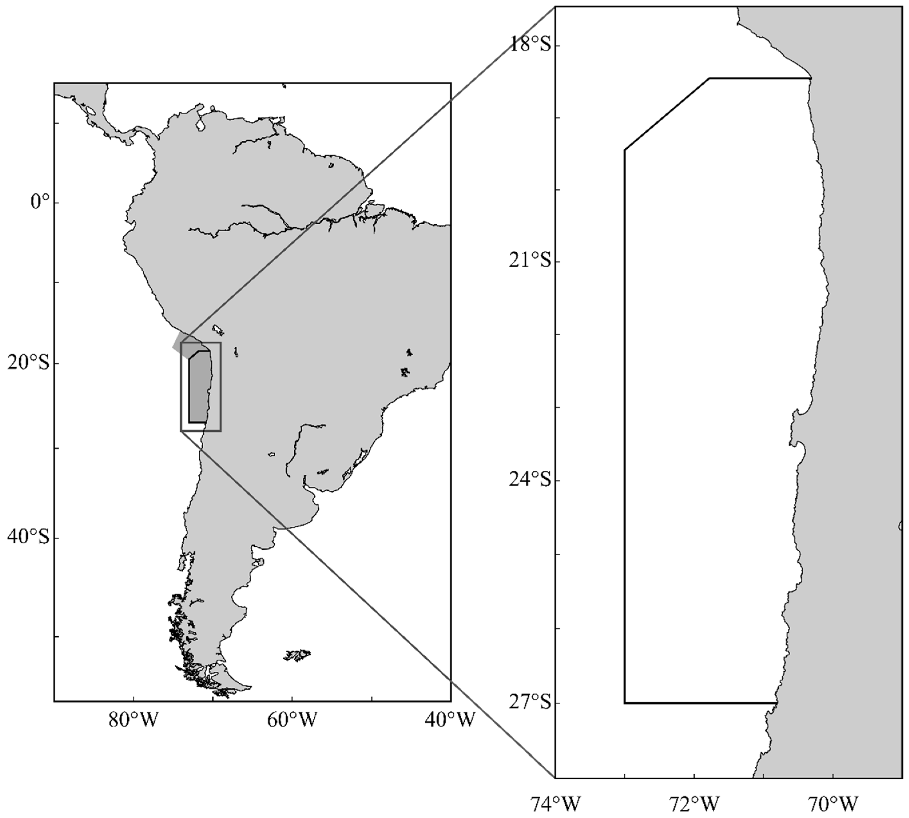
2.1. Fishery and Environmental Data

The georeferenced catch data of E. ringens per vessel and the daily trajectories of each ship were obtained from the database of the fishing company Corpesca S.A., which owns a fleet of 23 out of 33 vessels that comprise the industrial fleet in Northern Chile [7,8]. This database contains 1.5 million records for the 2003–2020 period, with a spatial resolution of 3 × 3 nm2. For the period 2003–2020, there was not differences in terms of the resolution and quality of the data in the database. The data included date (day, month, and year), geographic position where the vessel operated (latitude and longitude), georeferenced capture, and vessel identification. Each 3 × 3 nm2 cell was associated with a dichotomous variable to differentiate whether or not E. ringens was captured (0 = no catch; 1 = catch), independently of the catch volume. The absence data were determined from the full trajectory of the fishing vessels, under the assumption that vessels were searching for schools throughout the entire fishing trip. Each cell was also associated with the following daily oceanographic variables: sea surface temperature, salinity, depth of the mixed layer, currents, and sea height, which were obtained from the Copernicus Marine Environment Monitoring Service [16] and especially the product of the Global Analysis Forecast Phy 001 024 [17]. This source includes good-quality time series [18] produced using the NEMO physical model [19]. The study area ranged from 18° S to 26° S and from the coast to 73° W.

2.2. A forecasting Model Based on Artificial Neural Network

Data processing was performed in the Python programming language, using Tensorflow version 2.8 [20] and the Keras library [21] to implement the neural network. We used the daily trajectories of each ship, catches of E. ringens (with or without catch), and oceanographic variables to train a multi-layer perceptron, which is one of the neural network architectures most used for practical applications [14,22]. Eighty percent of the 1.5 million records were randomly assigned to training the model; the other 20% were used to validate it. Input data were standardized using the StandardScaler of Sklearn [23]. The neural network architecture was found using Auto-Keras [24]. The best architecture found consists of an input layer of nine neurons corresponding to the dimension of the input data (nine predictor variables). Two hidden (intermediate) layers were used with 1024 and 512 neurons, respectively, both with ReLU activation function [25]. The output layer of the model has a neuron with Sigmoid activation function [25], and the output is a value ranging from 0 to 1 for each 3 × 3 nm2 cell, which represents the catch probability in this cell. Since the case study corresponds to a binary classification, the loss function used was the BinaryCrossentropy [21]. We used Adam [26] as a neural network optimizer, with an initial learning rate of 0.001 that was configured to decrease throughout the training using the ReduceLROnPlateau keras function [27]. To avoid overfitting the model, a stopping criterion was implemented using the EarlyStopping function of Keras [28]. To analyze the importance of the variables, we applied the method proposed by [29], which assumes that the variables in which the weights of the neurons have greater variance in the training are the most relevant for prediction. The result of applying this method is the percentage support for each variable in predicting fishing grounds.

2.3. Model Validation

According to [30,31], the metrics used to evaluate neural network are the area under the receiving curve (AUC), precision (probability of catch in areas predicted by the model as PFGs), specificity (proportion of areas where there was no catch that the model detected correctly), recall (proportion of the catch areas detected by the model), and the false omission rate (FOR; the probability of catch in areas the model predicted as not apt for fishing). The AUC measures the relation between the true positive rate (TPR) and the false positive rate (FPR) [32]; it is 0 if the prediction is always wrong and is 1 when predictions are perfect [33,34,35]. The cross-validation of the model was performed to check if the results were the same independently of the data selected for training and validation. We used 10 random partitions of the database, varying the training and validation data.

2.4. Model Application

For each year of the 2003–2020 period, we simulated the catch probability of the fleet in the potential and non-PFGs, training a model for each year with the catch data and oceanographic variables for all the other years. A 3 × 3 nm2 cell was considered to be a PFG, if the probability determined by the model was greater than 0.5. The probability of the annual catch was calculated as:
Y C P = T C / T V ,
where Y C P is the catch probability for a year, T C is the number of 3 × 3 nm2 cells where E. ringens was caught, and T V is the total areas visited by the fleet.
To validate the neural network model as a daily predictive tool, we chose the 36 days (10% of the total days in a year) with greatest total captures in the study period (authors’ criterion). These 36 days were chosen only for graphic representation and to show examples of forecast maps of daily probabilities. This was used to generate a new model without using the information of the days selected for training, which was used to predict the probability of daily catch for each cell. Then, we mapped the probability of catch against the actual catches of the fleet.

3. Results

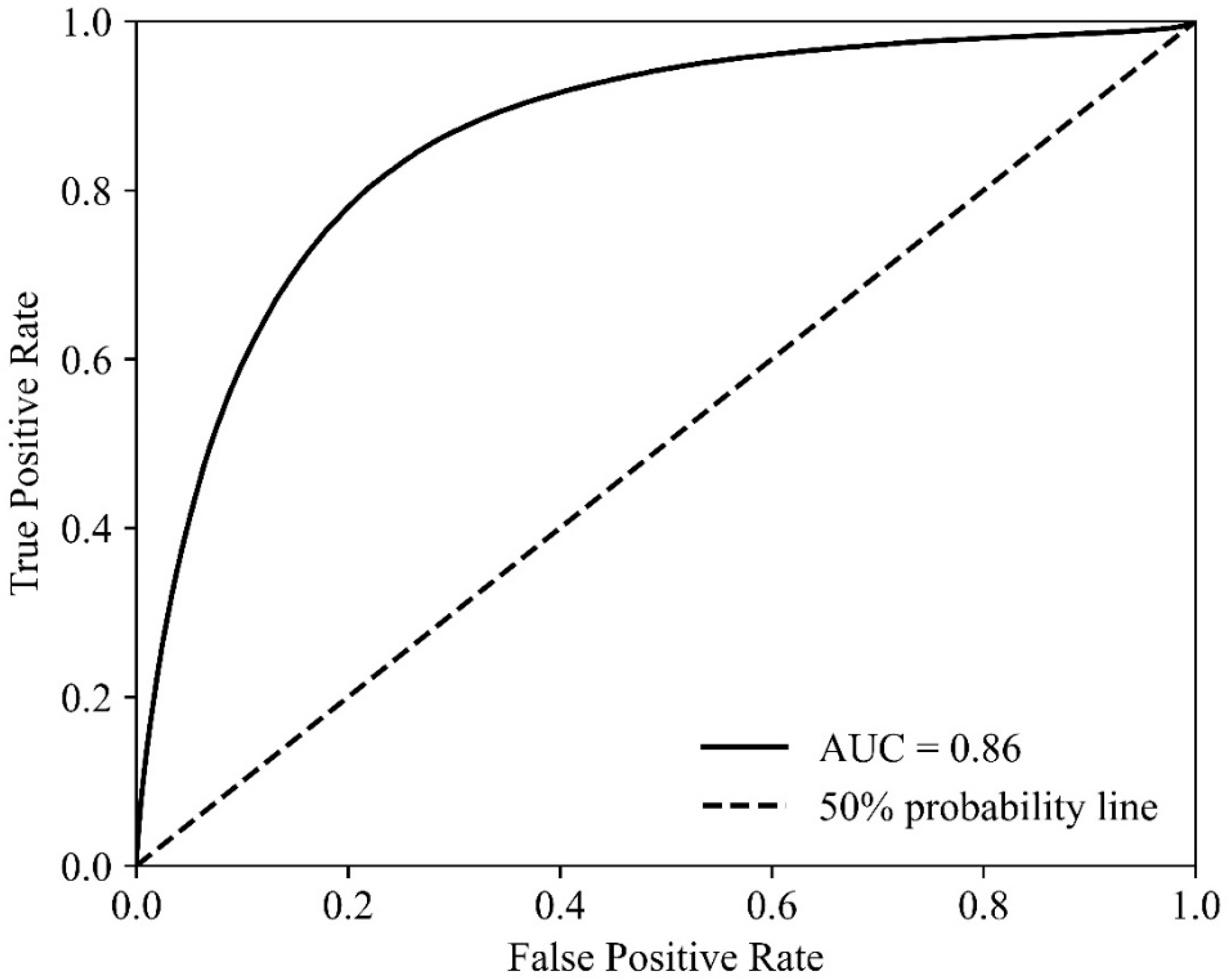
3.1. Performance of the Artificial Neural Network Forecasting Model

The AUCs were 0.848 for the model trained with 80% of the database and 0.86 for the test data (Figure 3). The test data included 302,182 3 × 3 nm2 cells visited by the fleet (Table 1); E. ringens was captured in 13,459 of them (4.45%), and thus, the catch probability was 0.0445. The model correctly identified 10,606 cells (78.8% of the cells where E. ringens was captured). Of the 85,341 cells predicted to have fish, catches were recorded in 10,606 (12%). Of the 216,841 cells predicted not to have fish, E. ringens was caught in 2853 (1.3%). The fishing effort (the number of cells fished by the fleet) in areas predicted not to have fish was 2.54 times that of the effort in areas predicted to have fish. The cross-validation of the model behaved similarly in all data partitions; the mean AUC was 0.84 (similar to that of the initial model test) and the recall was 0.79, both with a standard deviation of 0.01.
The most relevant variables for predicting PFGs were longitude (23%), depth of the mixing layer (18%), and latitude (15%), followed by sea surface temperature (12%), month (12%), sea height (9%), and salinity (9%). The least relevant variables were the zonal and meridional components of the marine currents (2% each); thus, these variables were excluded from the final model.

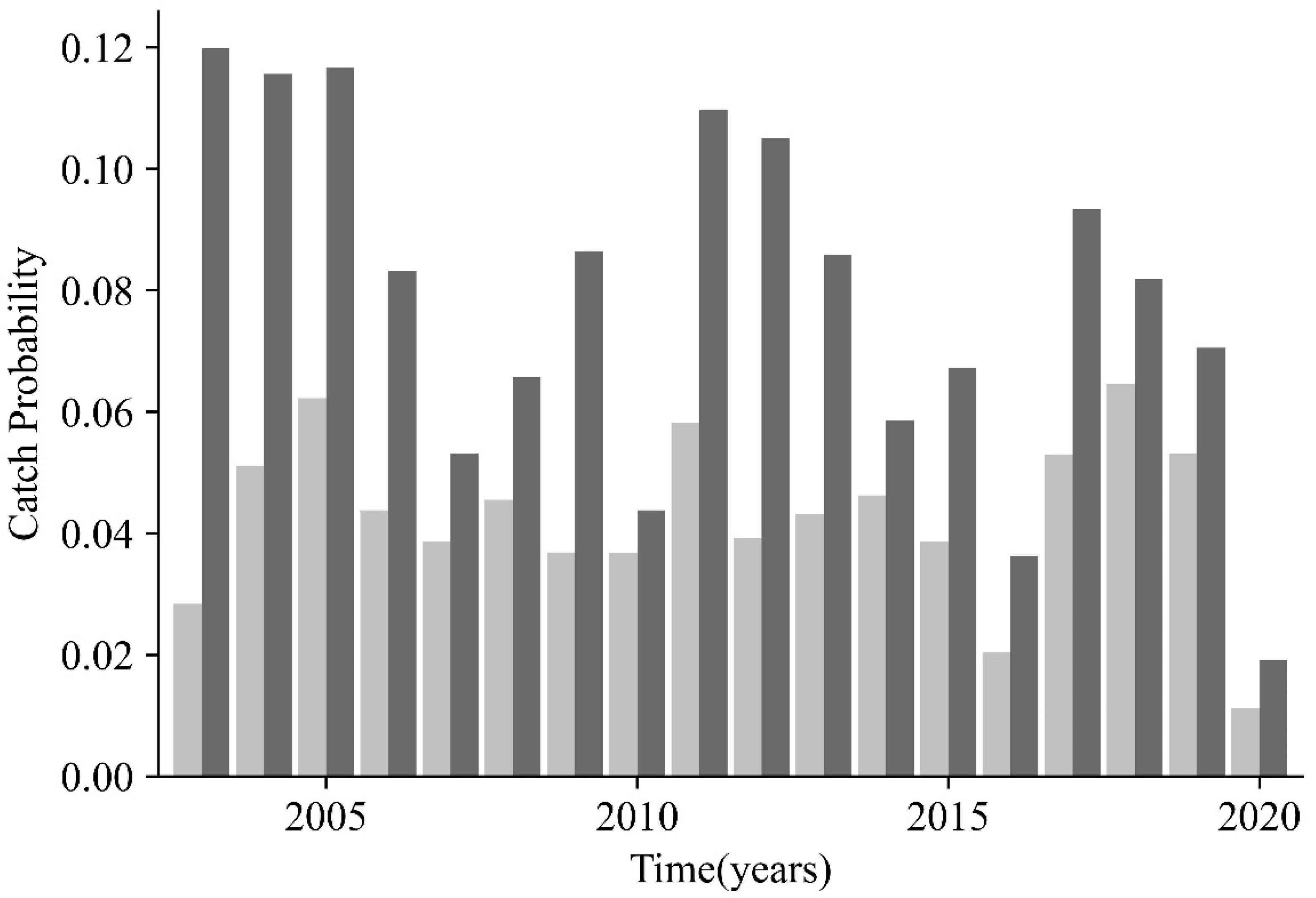
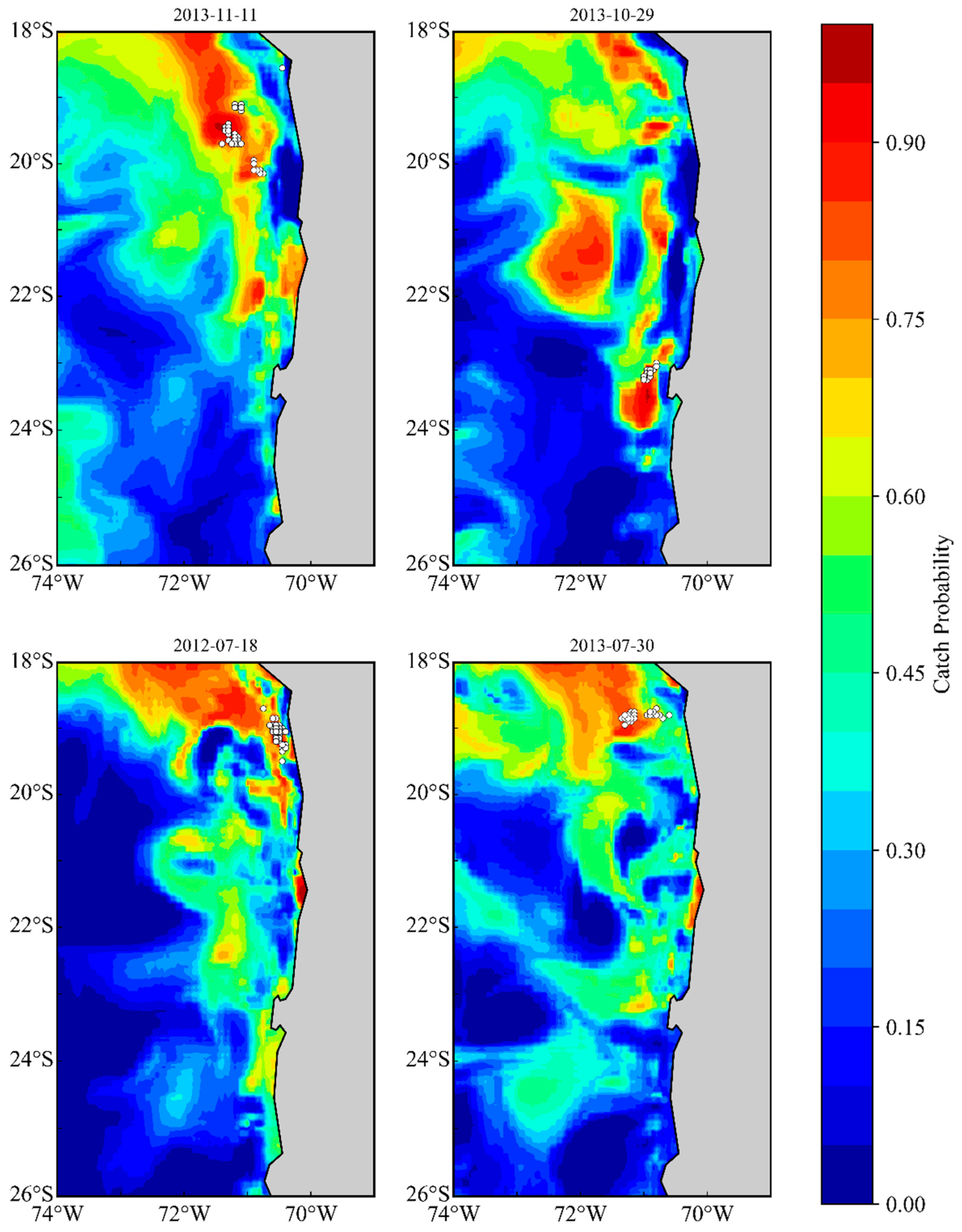
3.2. Model Application

Figure 4 shows the yield of the industrial purse seine fleet, expressed as YCP (Equation (1)) for all years studied. The mean catch probability in the PFGs was 88% greater than in the non-PFGs. The minimum difference was 19% (2010), and the maximum was 322% (2003).
Due to space limitations, Figure 5 shows the results of applying the model to the four days with the greatest catch of E. ringens in the entire time series. Table 2 shows a statistical summary of the behavior of the model for the 36 days of the greatest catch in the entire series. A larger number of areas with catches were within the areas of highest probability provided by the model. Seventy-five percent of the days had a precision greater than 0.12; this metric is equivalent to the catch probability in the areas predicted as PFGs by the model. The FOR, equivalent to the catch probability in areas predicted not to be PFGs, was below 0.05 in 75% of the cases. The recall is the fraction of fishing areas correctly detected by the model, and it was above 0.7 in 75% of the cases.

4. Discussion

The use of a neural network model to predict PFGs of E. ringens in Northern Chile proved to be an interesting method with practical applications. Predicting fishing grounds has been a great challenge for Chile and Latin America, due to which many efforts have made [36,37,38,39,40]. Although Chilean efforts have shown satisfactory results [37,39,40], they used oceanographic satellite information, which are instantaneous moments of the ocean state that do not allow temporal projection of these conditions in the short term. It is also unknown if these studies would have practical applications for the administration of the fleet.
Nieto et al. (2001) identified PFGs for E. ringens in 1999; 67% of the actual catch areas were among those the model identified (this metric is equivalent to recall, which is used in this study). Silva et al. (2002) [38], Yáñez et al. (2004) [39], and Silva et al. (2012) [40] used a similar methodology to identify PFGs of E. ringens, obtaining a 74% recall, which is comparable to the 79% recall obtained by us in the cross-validation and mean of 76% for the 36 days, of which 50% had a recall greater than 84% (Table 2). Our study identified and predicted 78.8% of the fishing grounds using a neural network (recall = 0.788) (Table 1 in Section 3.1). The AUC value of 0.84 indicates that the classification was very good according to the criteria of [41,42]. This result was compared favorably with the results of [43], who used a neural network model to predict the distribution of 14 species of freshwater fish and crustaceans in New Zealand; they reported AUC values of 0.63–0.88.
The neural network model applied in this study has the advantage that it may be implemented with few assumptions on the fishing and environmental data [13,14], showing better performance than conventional statistical models such as generalized linear models (GLMs) and generalized additive models (GAMs) [13,14,34,44]. The latter models require certain characteristics of the data, including linearity, normality, and heteroscedasticity [45]. However, these assumptions are unlikely to be fulfilled in real fishing situations, due to the lack of information in areas not explored by the fleet, the difficulty associated with the non-linearity of ecological processes (Tan and Beklioglu 2006), and the complex species-environment interactions (Wang et al. 2015). We found that the neural model also has limitations and disadvantages that need to be considered. For example, neural network models are considered as black boxes for which the prediction mechanism is not a transparent process or defined by an equation. Despite this, there are methods such as the one used in this study [29] to determine the importance of the variables in the predictions. The neural network requires data on presence and absence. The absence data were determined from the trajectory of the fishing vessels. As stated earlier, the assumption was that the vessels searched for schools during the full fishing trip, which is not necessarily correct. This assumption may have resulted in excessive absence zones and fewer presence zones. Therefore, the classes to be predicted are unbalanced, and the fishing probabilities are low. These could be improved in future studies by using fishing logbooks.
The neural network model applied in this study identified areas with oceanographic conditions favorable to the presence of E. ringens. However, this does not necessarily imply that schools will be present in those areas due to the existence of interactions with other species such as predation and competition [46]. This could explain why the model identified more PFGs than those where E. ringens was really caught (Table 1). However, the catch probability in the potential areas was greater than in the non-potential areas and greater than the fishing probability of the fleet if it visited all the areas (Table 1).
Similar to the report of Wang et al. (2015), in this study, the variables latitude and longitude were among the most important for identifying PFGs; In the case of E. ringens, their combined importance was 38%. The most relevant oceanographic variable was the depth of the mixing layer (18% of the variance). This variable is directly related to the vertical habitat of E. ringens, which in extreme events such as El Niño can expands to more than a 50 m depth; in this case, anchovy schools go deeper, making them less available for the purse seiners [5]. The annual simulation with the neural network model to recommend fishing grounds (Figure 4) showed that the probability in PFGs was greater than in the non-PFGs in all years. If the fleet had searched for schools of E. ringens in the areas recommended by the model, on average it would have had an 88% better probability of finding fish than in the non-recommended areas.
It must be emphasized that this study had millions of catch data provided by the fishing company Corpesca S.A., together with oceanographic predictions obtained from the Copernicus program. Corpesca S.A. is currently using this tool in Northern Chile to predict anchovy catch areas, which allows the fleet to self-regulate fishing effort better.
We concluded that the neural network model implemented in this study had 84% success in predicting PFGs for E. ringens. The real fishing areas where consistent with model predictions (Figure 5), which suggests that the model may be used to predict fishing grounds for E. ringens in Northern Chile. In addition, the model can help in reducing the fleet’s search effort for the target species and improving the fishing yield.

Author Contributions

Conceptualization, E.A., H.A. and S.N.; methodology, E.A. and H.A.; software, E.A.; validation, E.A.; formal analysis, E.A.; investigation, E.A. and H.A.; resources, E.A.; data curation, E.A.; writing—original draft preparation, E.A.; writing—review and editing, E.A., H.A. and S.N.; visualization, E.A. and H.A.; supervision, H.A. and S.N.; project administration, E.A.; funding acquisition, E.A. All authors have read and agreed to the published version of the manuscript.

Funding

This research was funded by Conicyt + Pai/Concurso Nacional Tesis de Doctorado en el Sector Productivo, Convocatoria 2019 + Folio (T7819110004) and partially funded by Centro COPAS Coastal ANID FB210021.

Data Availability Statement

The data that support the findings of this study are available from the corresponding author upon reasonable request.

Acknowledgments

This study was conducted using E.U. Copernicus Marine Service Information (https://doi.org/10.48670/moi-00016 (accessed on 24 June 2022)). E.A. thanks the “Doctorado en Ciencias con Mención en Manejo de Recursos Acuáticos Renovables (MaReA)” and Dirección de Postgrado from Universidad de Concepción (Chile) for the financial support provided through student scholarships. E.A. and H.A. thank the “Centro de Investigación Aplicada del Mar” (https://www.ciamchile.cl/ (accessed on 15 March 2021)) and Corpesca S.A (https://www.corpesca.cl/ (accessed on 15 March 2021)) for providing the data, offices, and staff support to carry out this research. S.N. acknowledges partial funding from Centro COPAS Coastal ANID FB210021.

Conflicts of Interest

The authors declare no conflict of interest.

References

  1. Barros, M.E.; Neira, S.; Arancibia, H. Trophic interactions in northern Chile upwelling ecosystem, Year 1997. Lat. Am. J. Aquat. Res. 2014, 42, 1109–1125. [Google Scholar] [CrossRef]
  2. Medina, M.; Arancibia, H.; Neira, S. Un modelo trófico preliminar del ecosistema pelágico del norte de Chile (18°20′ S–24°00′ S). Invest. Mar. 2007, 35, 25–38. [Google Scholar] [CrossRef]
  3. Espíndola, F.; Quiroz, J.C.; Böhm, G.; Leiva, F.; Aros, J.A. INFORME 2 ESTATUS. Convenio de Desempeño 2017. Estatus y posibilidades de explotación biológicamente sustentables de los principales recursos pesqueros nacionales Año 2018: Anchoveta XV-II Regiones. Inst. Fom. Pesque 2018. [Google Scholar] [CrossRef]
  4. Silva, C.; Andrade, I.; Yáñez, E.; Hormazabal, S.; Barbieri, M.A.; Aranis, A.; Böhm, G. Predicting habitat suitability and geographic distribution of anchovy (Engraulis ringens) due to climate change in the coastal areas off Chile. Prog. Oceanogr. 2016, 146, 159–174. [Google Scholar] [CrossRef]
  5. Böhm, M.G.; Hernández, C.; Días, E.; Pérez, G.; Ojeda, R.; Cerna, F.; Valero, C.; Gómez, M.; Machuca, C.; Muñoz, L. INFORME FINAL. Convenio de Desempeño, 2016. Programa de seguimiento de las principales pesquerías pelágicas de la zona norte de Chile, XV–IV Regiones, Año 2016. Inst. Fom. Pesq. 2017. [Google Scholar]
  6. Dec. Ex. N° 22-2022 Modifica Dec. Ex. Folio 202100228 Establece Cuota de Captura de Unidades de Pesquería de Anchoveta y Sardina Española Zona Norte Sometidas a Licencias Transables de Pesca, Año 2022. (Publicado En Página Web 23-05-2022) (F.D.O. 25-05-2022)–SUBPESCA Normativa. Available online: https://www.subpesca.cl/portal/615/w3-article-114576.html (accessed on 27 June 2022).
  7. Memoria Corpesca. 2021. Available online: https://www.corpesca.cl/wp-content/uploads/2022/04/Memoria-Anual-Corpesca-2021.pdf (accessed on 27 June 2022).
  8. Memoria Camanchaca. 2021. Available online: https://www.camanchaca.cl/wp-content/uploads/2022/04/Camanchaca-Memoria-2021-web.pdf (accessed on 27 June 2022).
  9. NOAA Climate Prediction Center. Available online: https://origin.cpc.ncep.noaa.gov/products/analysis_monitoring/ensostuff/ONI_v5.php (accessed on 29 October 2020).
  10. Ley N° 19.713 Establece Como Medida de Administración el Límite Máximo de Captura por Armador a las Principales Pesquerías Industriales Nacionales y la Regularización del Registro Pesquero Artesanal; Subsecretaría de Pesca; Ministerio de Economía, Fomento y Reconstrucción: Santiago, Chile, 2001.
  11. Ley N° 19.822 Modifica la ley Nº 19.713, Incorporando las Unidades de Pesquería que Indica en las Zonas que Señala la Medida de Administración Límite Máximo de Captura por Armador; Subsecretaría de Pesca; Ministerio de Economía, Fomento y Reconstrucción: Santiago, Chile, 2002.
  12. Nammalwar, P.; Satheesh, S.; Ramesh, R. Applications of remote sensing in the validations of potential fishing zones (PFZ) along the Coast of North Tamil Nadu, India. Indian J. Mar. Sci. 2013, 42, 283–292. [Google Scholar]
  13. Wang, J.; Yu, W.; Chen, X.; Lei, L.; Chen, Y. Detection of potential fishing zones for neon flying squid based on remote-sensing data in the northwest Pacific Ocean using an artificial neural network. Int. J. Remote Sens. 2015, 36, 3317–3330. [Google Scholar] [CrossRef]
  14. Suryanarayana, I.; Braibanti, A.; Sambasiva Rao, R.; Ramam, V.A.; Sudarsan, D.; Nageswara Rao, G. Neural networks in fisheries research. Fish. Res. 2008, 92, 115–139. [Google Scholar] [CrossRef]
  15. Yáñez, E.; Plaza, F.; Gutiérrez-Estrada, J.C.; Rodríguez, N.; Barbieri, M.A.; Pulido-Calvo, I.; Bórquez, C. Anchovy (Engraulis ringens) and sardine (Sardinops sagax) abundance forecast off northern Chile: A multivariate ecosystemic neural network approach. Prog. Oceanogr. 2010, 87, 242–250. [Google Scholar] [CrossRef]
  16. Home | CMEMS. Available online: https://marine.copernicus.eu/ (accessed on 22 March 2022).
  17. Data | Copernicus Marine. Available online: https://resources.marine.copernicus.eu/product-detail/GLOBAL_ANALYSIS_FORECAST_PHY_001_024/INFORMATION (accessed on 22 March 2022).
  18. Legaloudec, O.; Desportes, C.; Levier, B. Quality information document for global sea physical analysis and forecasting product. Mercator Ocean. Q. Newsl. 2019, 1–100. [Google Scholar]
  19. Madec, G.; Bourdallé-Badie, R.; Bouttier, P.-A.; Bricaud, C.; Bruciaferri, D.; Calvert, D.; Chanut, J.; Clementi, E.; Coward, A.; Delrosso, D.; et al. NEMO Ocean Engine. 2017. Available online: https://zenodo.org/record/3248739#.Ys-BY4RBxPY (accessed on 27 June 2022).
  20. TensorFlow. Available online: https://www.tensorflow.org/ (accessed on 27 June 2022).
  21. Moolayil, J.; Moolayil, J.; John, S. Learn Keras for Deep Neural Networks; Springer: Berlin/Heidelberg, Germany, 2019. [Google Scholar]
  22. Bertrand, S.; Díaz, E.; Lengaigne, M. Patterns in the spatial distribution of peruvian anchovy (Engraulis ringens) revealed by spatially explicit fishing data. Prog. Oceanogr. 2008, 79, 379–389. [Google Scholar] [CrossRef]
  23. Sklearn.Preprocessing.StandardScaler–Scikit-Learn 1.1.1 Documentation. Available online: https://scikit-learn.org/stable/modules/generated/sklearn.preprocessing.StandardScaler.html (accessed on 27 June 2022).
  24. Jin, H.; Song, Q.; Hu, X. Auto-Keras: An Efficient Neural Architecture Search System. In Proceedings of the 25th ACM SIGKDD International Conference on Knowledge Discovery & Data Mining; Association for Computing Machinery: New York, NY, USA, 2019; pp. 1946–1956. [Google Scholar]
  25. Sharma, S.; Sharma, S.; Athaiya, A. Activation Functions in Neural Networks. Int. J. Eng. Appl. Sci. Technol. 2020, 4, 310–316. [Google Scholar] [CrossRef]
  26. Kingma, D.P.; Ba, J.L. Adam: A method for stochastic optimization. In Proceedings of the 3rd International Conference on Learning Representations, ICLR 2015, San Diego, CA, USA, 7–9 May 2015; pp. 1–15. [Google Scholar]
  27. ReduceLROnPlateau. Available online: https://keras.io/api/callbacks/reduce_lr_on_plateau/ (accessed on 27 June 2022).
  28. EarlyStopping. Available online: https://keras.io/api/callbacks/early_stopping/ (accessed on 27 June 2022).
  29. de Sá, C.R. Variance-based feature importance in neural networks. Lect. Notes Comput. Sci. 2019, 11828, 306–315. [Google Scholar] [CrossRef]
  30. Verma, S.; Rubin, J. Fairness Definitions Explained. Proc.–Int. Conf. Softw. Eng. 2018, 24, 1–7. [Google Scholar] [CrossRef]
  31. Wardhani, N.W.S.; Rochayani, M.Y.; Iriany, A.; Sulistyono, A.D.; Lestantyo, P. Cross-validation metrics for evaluating classification performance on imbalanced data. In Proceedings of the 2019 International Conference on Computer, Control, Informatics and Its Applications, Tangerang, Indonesia, 23–24 October 2019; pp. 14–18. [Google Scholar] [CrossRef]
  32. Hoo, Z.H.; Candlish, J.; Teare, D. What is an ROC curve? Emerg. Med. J. 2017, 34, 357–359. [Google Scholar] [CrossRef] [PubMed]
  33. Maina, I.; Kavadas, S.; Katsanevakis, S.; Somarakis, S.; Tserpes, G.; Georgakarakos, S. A methodological approach to identify fishing grounds: A case study on greek trawlers. Fish. Res. 2016, 183, 326–339. [Google Scholar] [CrossRef]
  34. Mateo, R.G.; Felicísimo, Á.M.; Muñoz, J. Modelos de distribución de especies: Una revisión sintética. Rev. Chil. Hist. Nat. 2011, 84, 217–240. [Google Scholar] [CrossRef]
  35. Zhang, X.; Saitoh, S.I.; Hirawake, T. Predicting potential fishing zones of japanese common squid (Todarodes pacificus) using remotely sensed images in coastal waters of South-Western Hokkaido, Japan. Int. J. Remote Sens. 2017, 38, 6129–6146. [Google Scholar] [CrossRef]
  36. Barbieri, M.A.B.; Yanez, E.R.; Farias, M.S.; Aguilera, R.H. Determination of probable fishing areas for the albacore (Thunnus Alalunga) in Chile’s central zone. Dig. Int. Geosci. Remote Sens. Symp. 1989, 4, 2447–2450. [Google Scholar] [CrossRef]
  37. Nieto, K.; Yánez, E.; Silva, C.; Barbieri, M.A. Probable fishing grounds for anchovy in northern Chile using an expert system. Int. Geosci. Remote Sens. Symp. 2001, 7, 2985–2987. [Google Scholar] [CrossRef]
  38. Silva, C.; Nieto, K.; Barbieri, M.A.; Yáñez, E. Expert systems for fishing ground prediction models: A management tool in the Humboldt ecosystem affected by ENSO. Investig. Mar. 2002, 30, 201–204. [Google Scholar] [CrossRef]
  39. Yáñez, E.; Silva, C.; Nieto, K.; Barbieri, M.A.; Martínez, G. Using satellite technology improve chilean purseine fishing fleet. Gayana 2004, 68, 578–585. [Google Scholar] [CrossRef]
  40. Silva, C.; Barbieri, M.A.; Yáñez, E.; Gutiérrez-Estrada, J.C.; Delvalls, Á. Using indicators and models for an ecosystem approach to fisheries and aquaculture management: The anchovy fishery and pacific oyster culture in Chile: Case studies. J. Aquat. Res 2012, 40, 955–969. [Google Scholar] [CrossRef]
  41. Ren-Yan, D.; Xiao-Quan, K.; Min-Yi, H.; Wei-Yi, F.; Zhi-Gao, W. The predictive performance and stability of six species distribution models. PLoS ONE 2014, 9, e112764. [Google Scholar] [CrossRef]
  42. Yusop, S.M.; Mustapha, M.A. Influence of oceanographic parameters on the seasonal potential fishing grounds of Rastrelliger kanagurta using maximum entropy models and remotely sensed data. Sains Malays. 2019, 48, 259–269. [Google Scholar] [CrossRef]
  43. Joy, M.K.; Death, R.G. Predictive modelling and spatial mapping of freshwater fish and decapod assemblages using GIS and neural networks. Freshw. Biol. 2004, 49, 1036–1052. [Google Scholar] [CrossRef]
  44. Tan, C.O.; Beklioglu, M. Modeling complex nonlinear responses of shallow lakes to fish and hydrology using artificial neural networks. Ecol. Modell. 2006, 196, 183–194. [Google Scholar] [CrossRef]
  45. Yudaputra, A.; Robiansyah, I.; Rinandio, D.S. The Implementation of Artificial Neural Network and Random Forest in Ecological Research: Species Distribution Modelling with Presence and Absence Dataset. In Proceedings of the 3rd SATREPS Conference, 2019. Available online: https://publikasikr.lipi.go.id/index.php/satreps/article/view/216 (accessed on 27 June 2022).
  46. Melo-Merino, S.M.; Reyes-Bonilla, H.; Lira-Noriega, A. Ecological niche models and species distribution models in marine environments: A literature review and spatial analysis of evidence. Ecol. Modell. 2020, 415, 108837. [Google Scholar] [CrossRef]
Figure 1. Stock of anchovy (Engraulis ringens (E. ringens)) distributed from Southern Peru to Northern Chile (16°–27° S). The right panel indicates the distribution of E. ringens in Northern Chile that is the study area covered by a neural network model applied to predict E. ringens fishing grounds.
Fishes 07 00204 g001
Figure 2. Annual landings of the industrial fleet that operates over the anchovy stock shared by Southern Peru and Northern Chile. Data were obtained from [3].
Fishes 07 00204 g002
Figure 3. Receiver operating characteristic curve of the evaluation of the neural network model on the test data for the fishery of anchovy (E. ringens) in Northern Chile.
Fishes 07 00204 g003
Figure 4. Annual catch probabilities of the fleet in the potential (dark bars) and non-potential (clear bars) fishing areas from the neural network model applied for the fishery of anchovy (E. ringens) in Northern Chile.
Fishes 07 00204 g004
Figure 5. Maps of catch probabilities predicted by the neural network model applied to the fishery of anchovy (E. ringens) in Northern Chile, for the four days with the greatest catch in the 2003–2020 period (the 36 days with the greatest catch were ranked, and the first four were displayed). White circles indicate where E. ringens was captured.
Fishes 07 00204 g005
Table 1. Results of applying the neural network model on the test data (not used for training) from the fishery of anchovy (E. ringens) and the oceanographic characteristics of the study area (Northern Chile). Tabulated values correspond to the numbers of cells.
Non-Potential Fishing GroundsPotential Fishing GroundsTotal
Areas visited216,84185,341302,182
Capture areas285310,60613,459
Probability0.0130.1240.045
Table 2. Summary of statistics describing the performance of the neural network model applied to the fishery of anchovy (E. ringens) in Northern Chile, considering the 36 days of the greatest catch in the entire series chosen as a study case.
nMeanStandard
Deviation
Minimun
Value
25%50%75%Maximum
Value
Precision360.2080.1360.0630.1210.1740.2420.654
False omission rate (FOR)360.0360.0280.0040.0120.0260.0540.11
Recall360.7640.2110.1250.7050.8440.9110.971
Publisher’s Note: MDPI stays neutral with regard to jurisdictional claims in published maps and institutional affiliations.

