Abstract
Salmon farming stands out from many other industries with its very high profitability, but it is also highly volatile. The main question is whether the profit of individual firms is stable, or whether profitable firms change from year to year. The purpose of this article is to apply the theory of profit persistence to answer this question for salmon farming in Norway. By using panel data from 2010 to 2019, available from public statistics, we study the relative deviation from the average profits. We estimate the speed of adjustment to the profit norm by using a dynamic GMM estimator. We find a high degree of convergence to the average profit among salmon farmers. For companies belonging to the group with below-average profit, there is a positive correlation between growth and profitability and a negative link between debt ratio and deviation of profit rate. Our finding is that although the Norwegian aquaculture industry has large profits, there is large volatility in the profits of this industry. This is useful knowledge for investors, lenders, public authorities and others who need to know something about the risk in the aquaculture industry.
1. Introduction
Farmed salmon production is an important segment of the world fish market today. Production takes place in relatively few countries, the main producer being Norway, with around half of all production [1]. Other important producer countries are Canada, Chile, the Faroe Islands, and the United Kingdom [2]. Climate and geographical conditions limit the potential areas for this kind of production. Salmon is a popular food choice among consumers worldwide and demand for it has increased. Due to supply limits, there has been a considerable rise in market price in the last decade; for instance, from 2012 to 2019, the price increased from EUR 3.50 to 6.00 per kilo [3]. During this period, there was a substantial fall in the value of the Norwegian currency, while production costs rose by less than the rise in the prices. As a result, salmon farming has become very profitable. At the same time, considerable concentration occurred primarily through acquisitions. From 1996 to 2018, the ten largest salmon farming companies’ share of the industry’s overall sales volume increased from 18.9 to 67.3 percent [4]. Many of the big firms are listed on the Oslo Stock Exchange (OSE). There has been a strong rise in the market values of salmon firms since 2012. The salmon stock price index on the OSE increased almost tenfold from 2012 to 2018 [5].
There are a large number of published articles addressing the market, cost structure, and profitability of Norwegian salmon farming. The study of Asche et al. suggests that volume shares and small companies have a significant positive impact on performance [6]. There are considerable risks associated with the production of farmed salmon; hence, there is great variation and uncertainty in the link between input and output in the manufacture of this product [7,8]. Critical factors for its operation are weather and temperature changes, fish deaths, illnesses, fish escapes, algae growth, and other harmful factors [6,9,10,11,12]. These factors can cause sizeable economic losses [2,13,14]. In addition, there are considerable variations in prices and exchange rates that create uncertainty [15,16,17]. Furthermore, there is significant uncertainty related to feed costs, which account for about half of total costs [2,4]. Licences and strict public regulations lead to limited opportunities to increase salmon production [18]. Despite its success, the production of farmed salmon is quite controversial in Norway due to environmental conditions, among other things [1,19].
With the characteristics of this sector, the question of whether one company can achieve higher profits than others over a longer period arises. Location, innovation, and good methods of managing risk can help some companies achieve good financial results during many consecutive years. Asche and Sikveland tested this by studying the development of earnings before interest rate and tax (EBIT) [20]. They concluded that there was little correlation between the profits from year to year and that the hypothesis of a random walk could not be rejected. The salmon-farming sector is heavily reliant on factors outside the specific firms sphere of control, from diseases in the farms to exchange-rate fluctuations.
Salmon farming stands out from most other industries due to its combination of high volatility and profitability. In the literature of profit persistency, there has been little focus on such cases. In this paper, we contribute to the literature by applying the theory of Mueller (1986) and Gibrat (1931) to this unusual industry. By analysing this outlier industry, we can learn about how industries with similar characteristics work. In particular, the results in this article can be applied to other exporting industries with high risk in production [21,22]. The year-to-year correlation of within-firm profit rates is measured in deviations from sector mean, meaning that sector-wide yearly variations are controlled for through a simple transformation of the main variable. We apply this variable by using a dynamic panel data methodology to estimate the persistency of profit rates, and thus to analyse the importance of firm-specific factors in salmon farming. More knowledge about the profitability of the sector will be useful for companies engaged in aquaculture, for lenders, and not least for the authorities in the assessment of various forms of regulation and tax design.
Fish farming involves a risk of disease or escape of fish. Increased density of fish farms leads to an increased risk of disease that can have serious consequences for the industry. For this reason, the industry is strictly regulated. It is the central authorities that grant or sell licenses. Each license gives a company a permit for a maximum of tonnes of biomass (the maximum allowable weight of all salmon). In southern Norway, this is 780 tonnes, while in northern Norway, where the risk of disease is lower, each permit is set at 900 tonnes. The number of licenses granted by the authorities thus indicates the capacity limit for the industry.
The fish-farming industry in Norway has an annual production that runs counter to the capacity limit set by the authorities. Increasing production by getting the authorities to issue more licenses is a process that takes a long time. The production is therefore inelastic. Due to inelastic supply, higher demand (see Figure 1, left) results in higher prices and increased profit among firms producing farmed salmon. Data from public statistics confirm this picture (see Figure 2, left). From 2012 to 2020, there has been a solid increase in the price of salmon measured in NOK (Norwegian Krone). There is a strong link between price and profit rate. High salmon prices have led to solid profits in the sector. Despite high prices and very good profitability from 2014 to 2020, growth has been limited (Figure 2, right). The demand has become less price-elastic over time [23]. Hence, fish farming stands out in profitability compared to many other sectors.
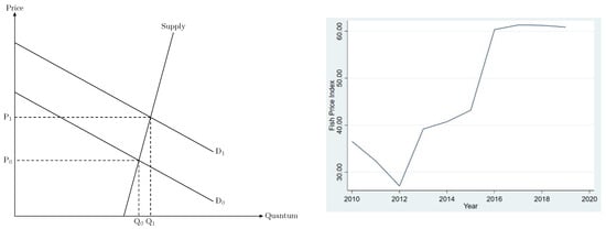
Figure 1.
The figure on the left shows weaker currency and higher demand (shift from demand from to ) have led to substantially higher prices (from to ) and profits since the supply curve is quite inelastic. The figure on the right shows the change in price of farmed fish. (Source: Norwegian public register for firms, Brønnøysund Register Center).
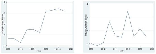
Figure 2.
The figure on the left shows the profit, and the figure on the right shows the growth among farmed salmon fishing in Norway from 2010 to 2019 (Source: Norwegian public register for firms, Brønnøysund Register Center).
It is of great interest to gain more knowledge about how profitability is distributed between companies and how it develops over time. See graphs showing the Fish Price Index (Figure 1, right), Industry Profits (Figure 2, left) and Industry Growth (Figure 2, right). Both growth and profit are related to prices, growth being the yearly change in revenue. The years 2010–2012 were characterised by negative growth, low profit, and falling prices. Prices increased after this, with a large jump in 2016, followed by stabilisation. The same jump and stagnation are seen in both industry profits and growth.
In recent years, there has been discussion of imposing a special tax on the aquaculture industry with reference to its high profits. This debate has lacked nuance due to little knowledge. Our contribution is as follows: Although the aquaculture industry can point to many companies with large profits, the financial result is very volatile. In the further debate on taxation, this should be taken into account [24].
2. Theory
2.1. The Persistence of Profit (PoP)
An important question is: if a company has higher or lower profit than the norm in a sector, will this gap be sustained or will the profit rate converge to the mean rate over time? An example of this is given in Figure 3. Many researchers have empirically analysed the degree of persistence of profit within different sectors [25,26]. These studies are mostly based on the work of Mueller [21].
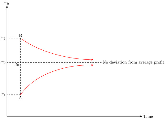
Figure 3.
The figure shows two companies, A and B, where the profit rate deviation from the average profit rate in the industry at time is and , respectively. The profit rate converges towards a state where there is no difference between the two companies’ profit rates and the industry average. The factor in Equation (2) measures the speed of adjustment to normal profit rate.
This paper will use the same procedure. expresses the profit for company i in period t. This is disturbed by cyclical variations, which calls for subtracting the mean profit rate for the sector () from firm profit rates, to obtain a measure robust to sector-wide economic forces. Furthermore, one divides the expression by the mean profit rate to produce a relative measure of profit-rate deviations. This gives the following equation for deviation of the profit rate of company i in the year t:
The simple autoregressive (AR1) model is:
where is a random error term for each firm at each time point of time. A value of above zero means this company has a higher than average profit rate for the sector, and vice versa if is negative. An interpretation of is the degree of profit persistence; that is, the degree to which firms carry over profitable years into the following year. Rational values vary between 0 and 1.0, but usually profit persistency lies in the range [26]. If is zero, firms that have above—or below—average profit rates for the sector in one year are expected to revert to the mean profit rate the following year. There is a rapid adjustment to the profit norm for this type of sector, and no profit persistency. A high value of reflects a sector in which firms keep their profit rates above the sector mean for extended periods, while a low value means that firms struggle to escape low-profitability times.
If , it does not make sense to talk about a sector mean. There is no convergence to a common mean. is thus a measurement or indicator of the short-run persistence parameter for profit. In the literature, an interpretation of the long-term steady-state equilibrium (permanent rent) is also used and is defined as:
where is the estimated constant.
Factors influencing the speed of adjustment to normal levels are market power, product differentiation and advertisement, advanced and heterogeneous products, entry barriers, cluster, advanced technology, and good leadership [21]. If any company has a strong position and manages to keep it, it may be able to secure high profits over a longer period. If the company convinces customers that its product is unique with high quality, willingness to pay can be high and competition from others will not be so strong. In particular, firms that manage strategically to build long-run relationships with customers are able to keep their profits high over a longer period. Customers may have a lack of knowledge, and the company’s management can succeed in portraying it as unique and sustainable. If, for economic or political reasons, there are significant barriers to entry, this could protect existing businesses. There may be high establishment costs, financial difficulties due to low equity, or considerable risk associated with the establishment of companies. If a company offers a product with advanced technology that is difficult for others to copy, this could secure the economy of the company. Companies that have a patent for a product can operate with very high profits over a long period of time. Conditions that lead to a rapid change to the normal level are a high degree of competition, homogenous products with simple technology, or limited entry barriers. From the neoclassical theory of the perfect market, new entrants will ensure that profits are competed away. Sectors with inelastic, volatile, or insecure production will tend to have low persistency of profits, as stable profits are hard to generate.
Even if one succeeds in achieving good results, it is not certain that they will persist. It depends on the situation. Existing empirical publications show that the level of profitability differs from the competitive norm and there is substantial sector variation. Bhangu reported a variation of short-run profit persistence from 0.2 to 0.6 depending on the sector [27]. The value of the coefficient was found to be high in consumer retailing, household and personal products, and health care. A moderate degree of profit persistence was observed in the capital-intensive industrials and information technology sectors. Companies in those sectors also managed to earn relatively high profits in the long run. Firms in financial sectors obtained the lowest score for profit persistence. A study by the McKinsey Global Institute confirmed a high value of among companies operating in idea-intensive fields such as the health sector and information technology [28]. Giotopoulos suggested a stronger degree of profit persistence in knowledge-intensive sectors compared to less knowledge-intensive production [29]. Gschwandtner and Hirsch found the profit persistence of the manufacturing sector to be higher than that of food processing companies [30]. Other drivers of above-average profitability are the size of the companies and the financial risk. Stronger competition will lower the profit deviation from the sector’s norm. It can be noticed that the empirical findings are mixed where culture, chosen country, and time have an influence on the results. For instance, Hirsch [26] found different values explaining the degree of profit persistence from Bhangu [27], suggesting a high persistence coefficient for the banking sector (near 0.4) and a very low one for the food sector (under 0.1). There are various factors that may influence the results of empirical studies. Opstad et al. estimated the profit persistence factor to be around 0.25 for the Norwegian restaurant industry [31].
2.2. Law of Proportionate Effect (LPE)
The empirical work is based on Gibrat’s Law [22]. This gives useful additional information for the analysis of enterprises and the profit level [32,33]. The model of LPE is:
where
is a constant, and is a random disturbance term. is the logarithmic value of size, measured by sales revenue, for firm i at time t.
Similarly to the literature on profit rate persistency, Gibrat’s LPE describes the trends of firms through an autoregressive parameter [22]. While Mueller’s profit persistence measures how fast firm-deviations from mean sector profit disappear [21], Gibrat’s law of proportional effect gives an estimate of market concentration dynamics. The law holds if , which means that the firms grow proportionately to their size, the best predictor of future size being past size. The firms follow a random walk, meaning that differencing firm size into firm growth, and estimating the equation as size on growth, gives the interpretation of firm growth being independent of firm size. If is larger than one, large firms grow faster than smaller ones and we observe market concentration in the sector. The opposite is true for , which indicates a mean reversion amongst firms, with smaller firms growing faster than larger ones. In the extreme case of , there would be perfect, and frictionless, competition.
The growth of firms cannot be described by perfect trends of, say, but will instead have years when they perform above or below their expected trend. The moving average parameter tells us whether performance above or below the expected trend in one year can predict growth that differs from the trend the next year. That is, will success or failure in one year lead to success or failure being the best predictor the next year? If so, will be significantly positive. If is negative, success in one year is expected to result in failure the next year, which would likely point to a sector characterised by volatility. A positive points to a sector with inertia, while means that firms that are off trend revert to trend within a year. That is, if there is no significant moving average component in firm trends, all shocks to size or growth are absorbed within a year and there are no spillover effects [33].
3. Research Questions
Having explained the salmon-farming market structure, we now focus on three key areas: profit, size, and firm-specific factors. By analysing profit persistence in salmon farming, we can measure the ability of firms to keep profits above the sector mean or, equivalently, the difficulty of catching up to mean profit. This parameter is understood as the speed of adjustment to the mean after a deviation from the mean profit rate. As far as we know, this is the first empirical analysis of Mueller’s profit persistence within this sector. Previous studies have found that industries with high levels of profitability tend to have high levels of profit persistency, but this might not be the case here.
- Research Question:
- Research question 1 is described in Equation (2) and asks: What is the degree of profit persistence for the Norwegian salmon farming industry?
To further analyse the trends of the salmon-farming industry, we estimate the growth dynamics of the sector’s firms. Whereas profit persistence is likely to be close to zero, the persistence of size is likely to be close to unity, which is what Gibrat’s Law predicts. If Gibrat’s Law holds, there is a random walk and the individual company’s relative growth is independent of the size of the company. In this paper, we apply the method used by Valenta et al. [33], which uses the level form of the dependent variable, in contrast to Asche and Sikveland [20], who use the difference. Importantly, the moving average component will be included. If it is not included, the estimated autoregressive parameter will be biased, capturing spillover effects.
- Research Questions:
- (2a) Does Gibrat’s Law hold for the Norwegian salmon-farming industry? (Equation (5)).
- (2b) Will failure or success be maintained the next period? (Equation (5)).
The third section of our paper investigates firm-specific variables which are believed to influence the profit rate deviations from the sector mean. Asche et al. found a positive correlation between the firm’s share of total sales and profitability [6]. There was also a positive link between working capital and performance, while operating leverage had a negative impact on profitability.
In Research Questions 1 and 3, we use the deviation of profit rates from the sector average as the dependent variable. When estimating firm-specific factors, we specify two models due to the large effect of salaries on profit rates. In previous literature, the cost of borrowing money tends to have negative impact on the profitability [34,35].
Hirsch and Valenta et al. reported a significant positive link between growth and profit rates [26,33]. Companies might take advantage of growth to achieve higher profits [25].
Controlling for firm-specific factors can have an impact on the level of profit persistence. According to the research of Giotopoulos, the effect might be stronger or weaker [29]. Based on known research, we postulate the following research questions:
- Research Questions:
- (3a) Is there a correlation between profitability and firm-specific factors?
- (3b) Does including business-specific characteristics of the sector have an impact on the level of profit persistency?
We have chosen to present Research Question 3 in a general form. Some factors can have positive effects, others negative ones, and there may be factors that do not have any effect. According to Yadav et al., there is mixed empirical evidence about the relationship between growth and profitability and between size and profitability [36]. If there are no economics of scale for salmon farmers, the link between profitability and size should be insignificant. Research has also found that growth is a determinant of profitability, and has a positive relationship [37]. Furthermore, the level of indebtedness has a negative influence on profit rates [38].
4. Methodology and Data
4.1. The Sample
The accounting information is available from a public register (Brønnøysund Register Center). From this list we obtained financial information for the last 10 years (see Table 1). The population consists of the 87 companies that have been in the market from 2010 to 2019. The total number of fish farms that existed in 2011 was 100. The sample that we used in our survey consists of the companies that have existed and submitted accounting information to the Brønnøysund Register Center from 2010 to 2019.

Table 1.
Descriptive statistics of the selected companies (1000 Norwegian Kroner).
It is rather unique that the mean profit rate for the firms in the sector is close to 25 percent (see Table 1). In other words, it is highly profitable. There are significant differences in size, and the largest company has a market share of over 10 percent. There is considerable variation between the companies in debt rate, working capital, and share of wage expenditures.
4.2. The Models
In line with research by Mueller [21], the simple autoregressive (AR) model is estimated to obtain the persistency of profits (see Equations (1) and 2), while Gibrat’s Law is estimated through an ARMA framework in accordance with Tschoegl [32] (see Equation (4)). The model is expanded to see company-specific factors that may explain deviations from normal profits. Several researchers have used this approach [39], but the choice of explanatory variables varies. The extended model is (M3):
where the growth rate is defined as:
The size is measured by market share. The working capital is a measure of the firm’s short-term liquidity. This factor can influence the firm’s decision about increasing production. With a shortage of working capital and investment, the firm probably needs loans to realise investments. Some of the company-specific factors have been analysed by Asche et al. [6]. A significant difference in this article compared to Asche et al. is that the dependent variable in this model is a deviation from the norm in the sector [6].
All models are estimated by applying the system GMM (general method of moments) framework introduced by Blundell and Bond [40]. They show that the estimator remains unbiased as the autoregressive parameter approaches unity, in contrast to the conventional GMM estimator, which is weak in this regard. Since the system GMM estimator remains unbiased, it is what is used in most applications of Mueller’s PoP and Gibrat’s Law. Discussions and applications of relevant estimators, their properties, and their weaknesses in the estimation of firm trends can be found in Valenta et al. [33]. As discussed by Hirsch and Gschwandtner, several researchers have used the GMM framework to estimate the persistency of profit, and it is the estimator that lends the most credibility in the field [41]. In line with Gschwandtner, we divide the sample into three subgroups depending on the initial profits of the companies for the first three years [25,42]. Group 1 (low profit) consists of companies that have initial profit rates below 20 percent. Firms with initial profit rates above 29 percent are placed in Group 3 (high profit). Group 2 contains firms in the middle with profits between 20 and 29 percent. A key question is whether there are any differences in the pattern among these three groups with regard to the degree of profit persistence and which factors characterise their differing profit rates.
To analyse the properties of the salmon-farming industry, we formulate three models. There are three important characteristic we wish to investigate in this article.
- The volatility in production due to illnesses in the salmon stock.
- The volatility in demand due to exchange-rate fluctuations.
- How the high profitability of the industry is distributed in face of the firms’ challenges with instability.
Figure 1 presents the supply and demand as inelastic supply with unstable demand on the left. Figure 1 shows the volatility and price sensitivity of the industry on the right. Figure 2 left shows the convergence towards the mean profit rate of firms differently hit by the exchange-rate appreciation of 2012.
Model 1 partly captures both the supply and demand by analysing the yearly revenue of the salmon farmers. In particular, the year-on-year effect of revenue deviation from its trend, the moving average component, is the parameter of interest.
Model 2 estimates the importance of firm-specific factors through the trend of profit-rate deviations from mean. This controls for cyclical effects, such as the exchange rate. This model captures how much firms can influence their rate of profit in the face of the volatile production of the industry.
Model 3 further examines these firm-specific factors by including specific variables. By extending model 2 into model 3, we can analyse whether specific strategies with regards to debt leverage and salary rates, for instance, can influence the success of salmon farmers. Since the salary of salmon farmers is quite inaccurately reported, we formulate two extended models, one with and one without the salary rate. The salary rate is also thought to be highly collinear with measures of size.
5. Findings and Discussion
5.1. Research Question 1 (PoP)
The degree of profit persistence is very low among the companies producing farmed salmon (Table 2). The value of is very close to zero, estimated as seven percent. This corresponds to less than a tenth of deviations from the profit mean expected to carry over in the next year. Of the subgroups, only the high initial profit persistence is significant, but it also represents less than a tenth of deviations. The initial differences in profit rates, which were particularly large as prices fell in 2012, disappeared very quickly as prices increased again. As seen from the graph in Figure 4, the differences were completely gone in 2016—at the highest point of the fish price index—though a slight difference reappeared later. This points to differences in firm practice, while any shock persistency is limited.
Table 2.
Result from Model 1 (profit persistence).
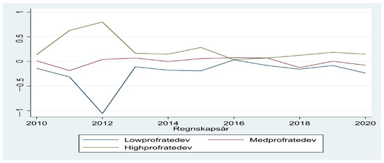
Figure 4.
The development of the gap in profits follows in large part the pattern outlined by Mueller (cf. Figure 3). Companies that perform differently from the average company converge to the norm during the period.
The answer to Research Question 1 is that companies that do better or worse than average do not retain this position for an extended period. This pattern is also clearly seen in the graphical representation (see Figure 4).
There are several possible factors that may explain why there is little degree of profit persistence in fish farming. Firstly, it is a rather homogeneous product with familiar technology. According to the approach of classical market theory, there is a tendency for the rate of profits to decline as technological convergence leads to homogeneity in production and product [43]. The main reason for this suggestion is the theory of competition, but empirical works about this issue give mixed results [44]. Since there is such a high average profit within fish farming, it is probably necessary to use another approach. Rumelt (1984) introduced the term “isolating mechanisms” [45]. By that, he means economic forces that protect existing businesses and prevent entry of new companies. Such mechanisms are obvious in salmon farming due to the conditions that characterise fish farming [7]. There is a requirement for a state license to operate in this sector and there are production restrictions. This explains why growth is so low despite the large profits (see Figure 1 and Figure 2) and why a high mean profit continues during a longer period. On the other hand, there is high risk associated with fish farming. There are many factors that influence the financial result (see the Section 1), as disease, lice, and temperature fluctuations affect the individual producer. A business may be lucky in one year through not being hit by such factors, but the situation may be completely different the following year. Therefore, the profit rate may vary widely over time. Since there is a requirement to change the location after a certain period, the benefit of good localisation will be limited if the business is analysed over a longer period. Furthermore, there are no special factors that indicate that a business can advertise a unique product and achieve good relationships with a particular customer group. Hence, the correlation between a company’s profits in one year and the following year is small [20]. Our analysis using model M1 confirms that there is no, or only a very small, degree of profit persistence (see Table 2).
However, there are some differences among the three groups in the permanent equilibrium values (See Table 3). Only for Group 3 is there a positive value. According to Gschwandtner, the value of is around zero for many companies (Group 2) [42]. However, a negative value is not a stable long-run equilibrium. This conclusion is based on the theory of perfect competition, however, where profits are close to zero in the long run. This is not the case for Norwegian salmon farming, where profit rates tend to be around 25 percent, meaning that firms can probably run profit rates below the sector mean for extended periods.
Table 3.
The value of (is calculated from the result in Table 2).
5.2. Research Question 2 (LPE)
The result of testing Gibrat’s Law confirms this conclusion or tendency (Research Question 2). The findings in Table 4 show that the hypothesis that (Equation (3)) is not rejected for the different groups. Since Gibrat’s Law holds, it means the companies follow a random walk. The company’s growth in the sector is independent of size, and there are no economies of scale effects. Which firms increase or decrease activity each year is coincidental—they follow a random walk.
Table 4.
Result from Model 2, ARMA (Gibrat’s Law).
For all groups, the moving average coefficient (Equation (4)) is strongly significant and negative with high values (above 0.5). This value is higher for Groups 1 and 3 than for Group 2, but not significantly so. The large negative moving average is a very interesting result, especially combined with the random walk trend of firm revenue. It indicates that a year with above-trend sales is expected to be followed by a year with below-trend sales and vice versa. That is, a successful year is expected to be followed by a year of failure. This overcorrection is estimated to be a little above half the size of the initial shock, as seen by the estimate .
Literature on the salmon industry discussing the high risk of the industry and the ambiguous link between input and output could explain this result [8,9]. This overcorrection mechanism of firm growth also explains the low degree of profit persistence in the industry, as profits are hard to maintain when faced with a volatile income stream, while a moving average component is likely.
5.3. Research Question 3: Firm-Specific Factors and Profitability
Our data suggest that the impact of firm-specific factors varies depending on the starting point. For Groups 2 and 3 (medium and high initial profits), none of the company-specific explanatory variables have a significant impact on the relative deviation from the average profit in the sector, though the estimate for the whole sample reflects that of the initially low-profit firms. There is obviously a different dynamic of profit development between Group 1 and the rest of the companies. Finding various degrees of profit persistence by using quantile regressions is in line with the report of Giotopoulos [29]. Our result suggests that having below-mean profit is stickier than having above-mean profit.
The result confirms that the market share or size of the companies did not affect the profit target (see Table 5). We did not find any correlation between working capital and the profit deviation. The literature discusses whether there can be a negative correlation between debt ratio and profitability [38]. Using the profit rate as the dependent variable, Asche et al. reported a positive association between the profit rate and working capital [6]. Afrifa and Padachi suggested that an optimal level of working capital exists [46]. Too much or too little will have a negative impact on the firm’s performance. The level of working capital is rather high for salmon farming. One explanation may be the high risk connected to this industry. In this study, we did not find any significant correlation between working capital and profitability. One reason may be that there is no clear correlation between the level of working capital and profit.
Table 5.
Result from Model 3a (without salary as explanatory variable).
Companies with high debt ratios have higher financial costs and there might be a time lag between investment and revenue. Therefore, one might expect a negative link between profit and debt ratios [6]. In this study, this effect appears for Group 1 and for the whole sample, but not for Groups 2 and 3.
Many studies have found a positive link between growth and profit rates [37,39]. If there is growth, a company can exploit this to improve the financial situation. This effect seems only to apply to companies belonging to Group 1 in this study. This is in line with Marris, who suggested that the link between growth and profitability is weak and mixed [47].
By including firm-specific explanatory variables, the value of changes from zero to 0.2 for Group 1 and is statistically significant (Research Question 3b). The speed of adjustment of short-run profit is slower in this extended model compared to the version presented in Table 2. For the whole sample, in this specification the adjustment factor is significant at around 0.1, which is a little stronger than that shown in Table 2. By controlling for factors such as the debt ratio and growth rate, there seems to be some degree of profit persistence for the companies with initial low profit rates, but not for Groups 2 and 3.
Notice that companies initially performing below the average need time to converge to the average profit, while companies achieving profits higher than the mean value are rapidly approaching the norm. Based on the available information, there is no obvious explanation for this asymmetry. However, the value of is rather low. Bhangu reported few cases with a speed of adjustment factor lower than 0.2. For most sectors, the value of was at least 0.3 [27]. With a significant impact only for Group 1 and with a value of around 0.1 for all companies, salmon farming still stands out with a high speed of adjustment to the norm compared to other sectors.
In Table 6, the salary share (of the total revenue) is included as an explanatory variable. This factor has a strongly negative impact on Groups 1 and 2 and almost no effect on Group 3. One possible explanation for this is that there is considerable rigidity in labour costs. For a company, those costs can be at the same level regardless of the level of production. If the company has lower staff turnover than expected due to illness and other factors, this will lead to a higher wage rate. This will statistically result in a negative correlation. Another explanation might be that companies affected by disease, fish death, and so on need extra employees to handle this situation. The result is lower profits and higher salary costs.
Table 6.
Result from Model 3b (including salary as explanatory variable).
6. Conclusions, Further Research, and Limitation
This paper investigated the degree of profit persistence among Norwegian salmon farmers. Previous literature showed a substantial variation in the speed of adjustment to normal profit between sectors. Despite the abnormally high profit level for companies within the salmon-farming sector, deviations from the mean value seem to be eliminated quickly.
Salmon farming is risky and the relationship between inputs and outputs is uncertain. With the same input, there can be a substantial deviation in the harvest. High production one year can be followed by low production the next year with the same level of input. The correlation between success in one year and in the following year is significantly negative. This might explain why firms follow a random walk and why Gibrat’s Law is not rejected. Our data show different pathways among the firms depending on the initial profit rates.
The main finding, however, is that even though the industry is highly profitable, the profitability does not persist through years for each company. This is useful information in forming tax schemes. This is an argument for having a flexible taxation which depends on the profitability of firms each year.
For companies belonging to the group with low profit, salary rates and debt ratios are negatively correlated to profitability, while growth is positively linked to this dependent variable.
Further research could analyse why there are substantial differences in the pathways of firms depending on their initial profit rates. A limitation of this paper is the duration of the sample and the lack of price strategy information. There is considerable variation between firms in pricing strategy, with the choice between spot and term prices. This could be a significant factor for explaining stability in profit rates.
Author Contributions
Writing—original draft, L.O., J.I. and R.V. All authors have read and agreed to the published version of the manuscript.
Funding
This research received no external funding.
Institutional Review Board Statement
Not applicable.
Informed Consent Statement
Not applicable.
Data Availability Statement
Not applicable.
Conflicts of Interest
The authors declare no conflict of interest.
References
- Hersoug, B. Why and how to regulate Norwegian salmon production?—The history of Maximum Allowable Biomass (MAB). Aquaculture 2021, 545, 737144. [Google Scholar] [CrossRef]
- Iversen, A.; Asche, F.; Hermansen, Ø; Nystøyl, R. Production cost and competitiveness in major salmon farming countries 2003–2018. Aquaculture 2020, 522, 735089. [Google Scholar] [CrossRef]
- Available online: https://fishpool.eu/fish-pool-european-buyers-index/ (accessed on 11 March 2022).
- Dennis, S.N.; Taranin, V. The Complexity of Reaching Further Production Growth in the Norwegian Salmon Farming Industry: A Two-Pronged APPROACH to qualitatively Evaluating Technological Development. Master’s Thesis, Norwegian School of Economics, Bergen, Norway, 2020. [Google Scholar]
- Misund, B.; Nygård, R. Big fish: Valuation of the world’s largest salmon farming companies. Mar. Resour. Econ. 2018, 33, 245–261. [Google Scholar] [CrossRef] [Green Version]
- Asche, F.; Sikveland, M.; Zhang, D. Profitability in Norwegian salmon farming: The impact of firm size and price variability. Aquac. Econ. Manag. 2018, 22, 306–317. [Google Scholar] [CrossRef]
- Asche, F.; Oglend, A. The relationship between input-factor and output prices in commodity industries: The case of Norwegian salmon aquaculture. J. Commod. Mark. 2016, 1, 35–47. [Google Scholar] [CrossRef]
- Asche, F.; Oglend, A.; Tveteras, S. Regime shifts in the fish meal/soybean meal price ratio. J. Agric. Econ. 2013, 64, 97–111. [Google Scholar] [CrossRef]
- Grefsrud, E.S.; Svås, T.; Glover, K.; Husa, V.; Hansen, P.K.; Samuelsen, O.B.; Stien, L.H. Risikorapport Norsk Fiskeoppdrett 2019-Miljøeffekter av Lakseoppdrett. Fisken og havet. 2019. Available online: https://imr.brage.unit.no/imr-xmlui/handle/11250/2640589 (accessed on 11 March 2022). (In Norwegian).
- Jensen, B.B.; Brun, E.; Fineid, B.; Larssen, R.B.; Kristoffersen, A.B. Risk factors for cardiomyopathy syndrome (CMS) in Norwegian salmon farming. Dis. Aquat. Org. 2013, 107, 141–150. [Google Scholar] [CrossRef]
- Pincinato, R.B.; Asche, F.; Bleie, H.; Skrudl, A.; Stormoen, M. Factors influencing production loss in salmonid farming. Aquaculture 2021, 532, 736034. [Google Scholar] [CrossRef]
- Taranger, G.L.; Karlsen, Ø; Bannister, R.J.; Glover, K.A.; Husa, V.; Karlsbakk, E.; Svås, T. Risk assessment of the environmental impact of Norwegian Atlantic salmon farming. ICES J. Mar. Sci. 2015, 72, 997–1021. [Google Scholar] [CrossRef] [Green Version]
- Abolofia, J.; Asche, F.; Wilen, J.E. The cost of lice: Quantifying the impacts of parasitic sea lice on farmed salmon. Mar. Resour. Econ. 2017, 32, 329–349. [Google Scholar] [CrossRef]
- Overton, K.; Dempster, T.; Oppedal, F.; Kristiansen, T.S.; Gismervik, K.; Stien, L.H. Salmon lice treatments and salmon mortality in Norwegian aquaculture: A review. Rev. Aquac. 2019, 11, 1398–1417. [Google Scholar] [CrossRef] [Green Version]
- Dahl, R.E.; Yahya, M. Price volatility dynamics in aquaculture fish markets. Aquac. Econ. Manag. 2019, 23, 321–340. [Google Scholar] [CrossRef]
- Asche, F.; Misund, B.; Oglend, A. The case and cause of salmon price volatility. Mar. Resour. Econ. 2019, 34, 23–38. [Google Scholar] [CrossRef]
- Baldursson, I.A. Price Hedging in Salmon Farming: Is Price Hedging a Viable, Profit Inducing Option for Salmon Farming Companies? Ph.D. Dissertation, Bifröst University, Bifröst, Iceland, 2021. [Google Scholar]
- Luthman, O.; Jonell, M.; Troell, M. Governing the salmon farming industry: Comparison between national regulations and the ASC salmon standard. Mar. Policy 2019, 106, 103534. [Google Scholar] [CrossRef]
- Olaussen, J.O. Environmental problems and regulation in the aquaculture industry. Insights from Norway. Mar. Policy 2018, 98, 158–163. [Google Scholar] [CrossRef] [Green Version]
- Asche, F.; Sikvel, M. The behavior of operating earnings in the Norwegian salmon farming industry. Aquac. Econ. Manag. 2015, 19, 301–315. [Google Scholar] [CrossRef]
- Mueller, D.C. Profits in the Long Run; Cambridge University Press: Cambridge, UK, 1986. [Google Scholar]
- Gibrat, R. Les Inégalits Économiques; Sirey: Paris, France, 1931. [Google Scholar]
- Xie, J.; Kinnucan, H.W.; Myrl, Ø. Demand elasticities for farmed salmon in world trade. Eur. Rev. Agric. Econ. 2009, 36, 425–445. [Google Scholar] [CrossRef]
- Norges Offentlige Utredninger 2019: 18. Oslo 2019. Available online: https://www.regjeringen.no/contentassets/207ae51e0f6a44b6b65a2cec192105ed/no/pdfs/nou201920190018000dddpdfs.pdf (accessed on 6 April 2022).
- Gschwandtner, A. Evolution of profit persistence in the USA: Evidence from three periods. Manch. Sch. 2012, 80, 172–209. [Google Scholar] [CrossRef]
- Hirsch, S. Successful in the long run: A meta-regression analysis of persistent firm profits. J. Econ. Surv. 2018, 32, 23–49. [Google Scholar] [CrossRef]
- Bhangu, P.K. Persistence of profitability in top firms: Does it vary across sectors? Compet. Rev. 2020, 30, 269–287. [Google Scholar] [CrossRef]
- McKinsey Global Institute. The New Global Competition for Corporate Profits. 2015. Available online: https://www.mckinsey.com/business-functions/strategy-and-corporate-finance/our-insights/the-new-global-competition-for-corporate-profits (accessed on 11 March 2022).
- Giotopoulos, I. Dynamics of firm profitability and growth: Do knowledge-intensive (business) services persistently outperform? Int. J. Econ. Bus. 2014, 21, 291–319. [Google Scholar] [CrossRef]
- Gschwandtner, A.; Hirsch, S. What drives firm profitability? A comparison of the US and EU food processing industry. Manch. Sch. 2018, 86, 390–416. [Google Scholar] [CrossRef] [Green Version]
- Opstad, L.; Idsø, J.; Valenta, R. The Dynamics of the Profitability and Growth of Restaurants; The Case of Norway. Economies 2022, 10, 53. [Google Scholar] [CrossRef]
- Tschoegl, A.E. Size, growth, and transnationality among the world’s largest banks. J. Bus. 1983, 56, 187–201. [Google Scholar] [CrossRef]
- Valenta, R.; Idsø, J.; Opstad, L. Evidence of a threshold size for Norwegian campsites and its dynamic growth process implications—Does Gibrat’s law hold? Economies 2021, 9, 175. [Google Scholar] [CrossRef]
- Eriotis, N.P.; Frangouli, Z.; Ventoura-Neokosmides, Z. Profit margin and capital structure: An empirical relationship. J. Appl. Bus. Res. (JABR) 2002, 18. [Google Scholar] [CrossRef] [Green Version]
- Nguyen, H.T.; Nguyen, A.H. The impact of capital structure on firm performance: Evidence from Vietnam. J. Asian Financ. Econ. Bus. 2020, 7, 97–105. [Google Scholar] [CrossRef]
- Yadav, I.S.; Pahi, D.; Gangakhedkar, R. The nexus between firm size, growth and profitability: New panel data evidence from Asia–Pacific markets. Eur. J. Manag. Bus. Econ. 2021, 31, 115–140. [Google Scholar] [CrossRef]
- Musah, A.; Gakpetor, E.D.; Pomaa, P. Financial management practices, firm growth and profitability of small and medium scale enterprises (SMEs). Inf. Manag. Bus. Rev. 2018, 10, 25–37. [Google Scholar] [CrossRef] [Green Version]
- Opstad, L.; Idsø, J.; Valenta, R. The degree of profit persistence in tourism industry. The case of Norwegian campsites. Int. J. Econ. Bus. Adm. 2021, 9, 140–155. [Google Scholar] [CrossRef]
- Zouaghi, F.; Hirsch, S.; Garcia, M.S. What drives firm profitability? A multilevel approach to the Spanish agri-food sector. In Proceedings of the 56th Annual Conference, Bonn, Germany, 28–30 September 2016. No. 873-2016-60917. [Google Scholar]
- Blundell, R.; Bond, S. Initial conditions and moment restrictions in dynamic panel data models. J. Econom. 1998, 87, 115–143. [Google Scholar] [CrossRef] [Green Version]
- Hirsch, S.; Gschwandtner, A. Profit persistence in the food industry: Evidence from five European countries. Eur. Rev. Agric. Econ. 2013, 40, 741–759. [Google Scholar] [CrossRef] [Green Version]
- Gschwandtner, A. Profit persistence in the ‘very’ long run: Evidence from survivors and exiters. Appl. Econ. 2005, 37, 793–806. [Google Scholar] [CrossRef]
- Harris, D.J. On the classical theory of competition. Camb. J. Econ. 1988, 12, 139–167. [Google Scholar] [CrossRef]
- Bahçe, S.; Eres, B. Components of differential profitability in a classical/Marxian theory of competition: A case study of Turkish manufacturing. In Alternative Theories of Competition; Routledge: London, UK, 2012; pp. 251–288. [Google Scholar]
- Rumelt, R.P. Towards a strategic theory of the firm. Compet. Strateg. Manag. 1984, 26, 556–570. [Google Scholar]
- Afrifa, G.A.; Padachi, K. Working capital level influence on SME profitability. J. Small Bus. Enterp. Dev. 2016, 23, 44–63. [Google Scholar] [CrossRef]
- Marris, R.; Maclean, I.; Bernau, S. The Economics of Capital Utilization; Macmillan: London, UK, 1964. [Google Scholar]
Publisher’s Note: MDPI stays neutral with regard to jurisdictional claims in published maps and institutional affiliations. |
© 2022 by the authors. Licensee MDPI, Basel, Switzerland. This article is an open access article distributed under the terms and conditions of the Creative Commons Attribution (CC BY) license (https://creativecommons.org/licenses/by/4.0/).