Spatiotemporal Analysis of Light-Fishing Vessel Operations in the Arabian Sea Based on Nighttime Light Remote Sensing

Abstract

A comprehensive understanding of the spatial dynamics and operational characteristics of fishing activities in the Arabian Sea is critical for effective marine management and regional resource conservation. Based on VIIRS/DNB nighttime light imagery from 2017 to 2022 and the YOLOv11 model, this study presents an applied observational pipeline for the spatial extraction of fishing vessel positions. Spatial statistical methods were employed to analyze the operational patterns of light-fishing fleets, and habitat niches were identified by integrating marine environmental data. The results indicate that: (1) The YOLOv11 model achieved a precision (P) of 0.966, a recall (R) of 0.954, and a mean average precision (mAP) of 0.969. Under clear-sky and thin-cloud conditions, it demonstrated superior detection accuracy compared to existing VBD (VIIRS Boat Detection) products. (2) Through Kernel Density Hotspot Analysis (KDHSA), the primary spatial distribution of the light-fishing fleet was delineated. Fishing Operation Areas (FOAs) exhibited a pronounced seasonal “clustering–diffusion–re-clustering” pattern. The Center of Effort (CoE) generally followed a counter-clockwise migration trajectory, though a clockwise shift was observed during the 2019–2020 fishing season. (3) Random Forest analysis identified dissolved oxygen at 200 m (DO200), sea surface height (SSH), and temperature at 200 m (T200) as the primary predictive environmental features associated with vessel distribution. The core spatial ranges associated with high vessel density were 9.5–14.9 mmol⋅m⁻³ for DO200, 0.24–0.36 m for SSH, and 17.3–18.0 °C for T200. Notably, the statistical contribution of subsurface factors significantly exceeded that of sea surface temperature (SST). Future research should integrate ship position data with fishery biological data to further explore the drivers of FOA variations. This study provides a scientific basis for the sustainable management and rational development of marine resources in the Northwest Indian Ocean.

1. Introduction

Global capture fisheries are currently facing unprecedented challenges, as intensifying fishing pressure threatens the resilience of marine ecosystems and the sustainability of fishery resources [1]. In this context, a profound understanding of the spatial distribution and operational characteristics of fishing activities is essential for implementing effective marine management and regional resource conservation. Among various fishing techniques, light-assisted fishing has emerged as one of the most efficient and successful methods globally, characterized by high harvest efficiency, strong selectivity, and relative energy economy [2].

The Arabian Sea, located in the Northwest Indian Ocean, exhibits high primary productivity driven by complex monsoonal dynamics [3]. Since 2017, the operational scale of the Chinese light-fishing fleet—primarily composed of light-seiners and squid jiggers—has expanded significantly in the high seas of this region. These fleets predominantly target the Sthenoteuthis oualaniensis (purpleback flying squid), a commercially vital species that accounted for over 80% of the total catch in the region between 2017 and 2020 [4].

Research into these cephalopod resources dates back to the mid-1960s. Systematic surveys conducted by Soviet and Japanese scientists between the 1960s and 1990s identified the Northern Arabian Sea as a high-abundance zone, where fleet aggregations typically coincided with hydrological fronts and specific favorable temperature ranges, generally exceeding 20 °C [5,6,7]. Since China initiated exploratory surveys in 2003, the understanding of S. oualaniensis distribution in the Northwest Indian Ocean has evolved from preliminary resource mapping to refined spatial modeling [6,7,8,9,10,11,12,13]. Early investigations indicated that areas with high Catch Per Unit Effort (CPUE) were concentrated between 14–16° N and 60–63° E [6,10,11]. With the continuous expansion of the Chinese fleet, subsequent studies integrated multi-source fishery logbooks with statistical frameworks such as Generalized Additive Models (GAM) and Random Forests (RF) to clarify key environmental thresholds. These studies identified an optimal Sea Surface Temperature (SST) range of 25.0 °C to 28.5 °C, alongside other critical drivers including chlorophyll-a concentration (0.2–0.5 mg·m⁻³) and dissolved oxygen (DO) levels [14,15,16,17,18]. Analyses of the fleet’s “Center of Effort” (CoE) have revealed a rhythmic, counter-clockwise seasonal migration pattern [19,20].

Despite these advancements, a significant gap remains in the objective and continuous monitoring of light-fishing dynamics in the Arabian Sea. Current research relies heavily on fishery logbooks and sporadic survey data, which are often subject to subjective reporting biases and incomplete spatial coverage. This limitation is particularly acute for vessels with irregular Automatic Identification System (AIS) signal transmissions.

Since the late 1970s, Nighttime Light (NTL) remote sensing has emerged as a unique and reliable technical solution for monitoring light-assisted fishing activities [21]. Early studies utilized Defense Meteorological Satellite Program/Operational Linescan System (DMSP/OLS) data, employing various threshold segmentation methods—such as manual segmentation and Otsu’s method—to identify FOAs, estimate fishing effort (vessel counts), and analyze fish migration patterns globally [22,23,24,25,26,27,28,29,30]. The field advanced further with the launch of the Suomi National Polar-orbiting Partnership (SNPP-VIIRS) satellite; its Day/Night Band (DNB) offers superior radiometric resolution, enabling the detection of smaller and more dispersed light sources [31]. However, the VIIRS Boat Detection (VBD) product developed by the Earth Observation Group (EOG) remains susceptible to interference from lunar irradiance and cloud optical thickness, leading to frequent false detections during full moon periods [31,32]. To overcome the inherent limitations of manual rules, deep learning-based Artificial Intelligence (AI) has recently been introduced to enhance detection capabilities through multi-scale feature extraction [33]. While frameworks such as DNA-net [34], YOLOv5 [35,36], and YOLOv8 [37] have improved performance, their ability to accurately segregate targets remains constrained under heavy cloud cover or in dense vessel clusters. As one of the latest iterations in the YOLO series, YOLOv11 integrates an enhanced backbone-neck architecture and updated lightweight modules with fused attention mechanisms. These improvements significantly optimize the balance between inference speed and detection accuracy, particularly enhancing the perception and localization of tiny or blurred targets in complex radiative backgrounds [33]. To date, no study has utilized NTL remote sensing data to identify light-fishing FOAs and analyze their spatiotemporal patterns in the Arabian Sea.

The objectives of this study are as follows: (1) to extract light-fishing vessel positions in the Arabian Sea from 2017 to 2022 using VIIRS/DNB imagery and the YOLOv11 architecture, evaluating the model’s accuracy and robustness across diverse radiative backgrounds; (2) to delineate the primary spatial distribution of the fleet using Kernel Density Hotspot Analysis (KDHSA), map the frequency distribution of FOAs, and derive the seasonal migration trajectories of the CoE; and (3) to identify the marine environmental factors influencing the spatiotemporal distribution of FOAs using Random Forest models, characterizing seasonal environmental preferences. By applying advanced deep learning to NTL imagery and integrating multi-parameter oceanographic analysis, this study provides a critical scientific basis for the sustainable management and rational development of cephalopod resources in the Northwest Indian Ocean.

2. Materials and Methods

2.1. Data Sources and Study Area

The study area focuses on the high seas of the Arabian Sea, specifically encompassing the region north of 10° N. To conduct a spatiotemporal analysis of light-fishing vessels, this study integrated three primary categories of data: Nighttime Light (NTL) imagery, Vessel Monitoring System (VMS) data, and marine environmental parameters.

2.1.1. Nighttime Light (NTL) Remote Sensing Data

The Day/Night Band (DNB) dataset from the Visible Infrared Imaging Radiometer Suite (VIIRS) served as the primary data source for detecting light-fishing vessels. The data, spanning from 1 September 2017 to 30 April 2022, were obtained from the Comprehensive Large Array-data Stewardship System (CLASS) of the National Oceanic and Atmospheric Administration (NOAA) (https://www.aev.class.noaa.gov/saa/products/welcome, accessed on 1 April 2026). The high sensitivity of the DNB sensor enables the effective capture of high-intensity artificial lighting emitted by fishing vessels during nighttime operations.

2.1.2. Vessel Monitoring System (VMS) Data

To provide “ground truth” for NTL-based detection and to support the construction of a robust object detection dataset, this study utilized Vessel Monitoring System (VMS) data. These data were provided by the Technical Group for the Trawl-Purse Seine Fishery within the Distant-water Fishery Society of China. The VMS dataset contains high-precision trajectory information, including geographic coordinates and timestamps, for Chinese light-fishing vessels within the study area. These records were employed both to validate the accuracy of the NTL imagery extraction and as expert-labeled data for training the deep learning models.

2.1.3. Marine Environmental Data

Research indicates that factors such as sea surface temperature (SST) [11], chlorophyll-a (Chl-a) [18], dissolved oxygen (DO) [18], sea surface height (SSH) [7], and ocean currents [38] significantly influence the distribution of target species for light-seining in the Arabian Sea. These variables are categorized into three functional dimensions: (1) thermodynamic conditions, (2) biogeochemical indicators, and (3) physical oceanographic characteristics. Furthermore, S. oualaniensis exhibits distinct diel vertical migration, ascending to the surface to forage at night and descending to depths exceeding 200 m at dawn [5]. In this study, these variables were utilized to investigate the environmental drivers influencing the spatial distribution of fishing activities. A total of 17 variables, including subsurface parameters at depths of 50 m, 100 m, and 200 m, were incorporated into a Random Forest (RF) model to assess their relative contributions to fishing intensity. Multi-source marine environmental variables were obtained from the Copernicus Marine Service (CMEMS, https://marine.copernicus.eu accessed on 1 April 2026); their detailed definitions, abbreviations, and units are summarized in

Table 1. Summary of marine environmental variables.

Category	Environmental Variable	Abbreviation	Units	Depth/Description
Thermodynamic	Sea Surface Temperature	SST	°C	Surface
	Subsurface Temperature	T50, T100, T200	°C	50 m, 100 m, 200 m
Biogeochemical	Chlorophyll-a Concentration	Chl-a	mg⋅m−3	Surface
	Primary Production	PP	mg⋅C⋅m−2⋅d−1	Surface
	Dissolved Oxygen	DO	mmol⋅m−3	Surface
	Subsurface Dissolved Oxygen	DO50, DO100, DO200	mmol⋅m−3	50 m, 100 m, 200 m
Physical	Sea Surface Salinity	SSS	PSU	Surface
	Subsurface Salinity	S50, S100, S200	PSU	50 m, 100 m, 200 m
	Mixed Layer Depth	MLD	m	-
	Sea Surface Height	SSH	m	-
	Surface Current Velocity	SCV	m⋅s−1	Surface

.

2.2. Overall Methodological Framework

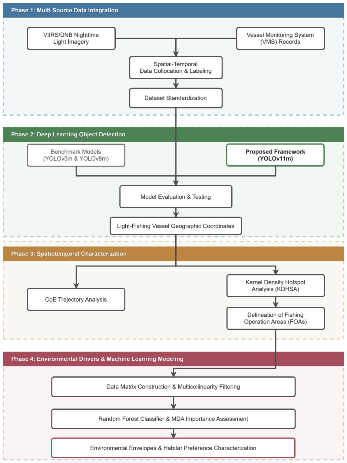
The methodological framework of this study comprises four interconnected phases: data integration, object detection, spatiotemporal characterization, and environmental correlation analysis (Figure 1). Initially, multi-source data, specifically Vessel Monitoring System (VMS) records and VIIRS/DNB imagery, are integrated. Within this workflow, the VMS data serve as the “ground truth” reference for constructing a robust training dataset and validating detection accuracy, while the DNB imagery acts as the primary source for identifying light-fishing vessels. Subsequently, a deep learning-based object detection model, YOLOv11, is implemented to extract the geographic coordinates of the vessels. These extracted positions are then utilized to quantify fishing intensity through the CoE and Kernel Density Hotspot Analysis (KDHSA), the latter of which is primarily used to delineate FOAs. Finally, the spatiotemporal dynamics are synthesized with marine environmental factors to perform an environmental correlation analysis, aimed at investigating the underlying patterns and drivers of FOA variations.

2.3. Light-Fishing Vessel Detection Model and Accuracy Evaluation

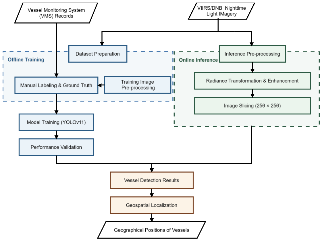
To bridge the gap between raw satellite imagery and high-precision fishing vessel distribution data, the detection and localization process established in Section 2.2 was further expanded into a comprehensive workflow (Figure 2).

2.3.1. Dataset Preparation and Model Training

The initial stage involved dataset preparation aimed at establishing a high-quality benchmark. To extend the dynamic range and accentuate low-radiance fishing vessel pixels against the dark background, a “radiance transformation and enhancement” technique was applied. Radiance values L were scaled and transformed using a logarithmic function:

L’ = log10(L × 10⁹)

(1)

where L represents the original radiance value and L’ denotes the transformed value.

Subsequently, the imagery was segmented into grayscale image tiles (256 × 256 pixels). Guided by concurrent VMS tracking data from 2020, manual annotation and ground truth generation were performed using the LabelImg tool (Version 1.8.6), focusing on active operational grids. This process produced a specialized target detection dataset comprising 305 sub-image tiles and 4988 distinct fishing vessel targets. To ensure spatial and environmental representativeness, the dataset encompasses a comprehensive suite of complex marine scenarios, including varying lunar phases, diverse background sea-surface noise levels, and heterogeneous atmospheric conditions defined by different cloud top heights, cloud thicknesses, and cloud optical depths. Finally, the dataset was partitioned into training, validation, and testing sets with a ratio of 7:2:1.

Model training was executed within a Windows environment on a dedicated workstation equipped with an Intel Xeon W-2245 CPU (@ 3.90 GHz) and an NVIDIA RTX A5000 GPU with 24 GB VRAM. The YOLOv11 architecture was trained for 1000 epochs utilizing a batch size of 32. To ensure stable gradient descent and prevent overfitting, the initial learning rate was optimized at 0.005, which smoothly decayed to a final learning rate factor of 0.01 via a cosine annealing scheduler, coupled with an L2 regularization weight decay coefficient of 0.0005. To fortify model generalization under varying maritime background noises, a rigorous hybrid data augmentation pipeline was deployed during training; this included standard Mosaic augmentation, mixed with Copy-Paste (30% probability) and MixUp (15% probability) techniques. These were further combined with fine-grained geometric transformations (a scaling factor of 0.9 and perspective transformation of 0.001) and color perturbations (±1.5% hue, ±70% saturation, and ±40% brightness adjustment) to prevent the network from memorizing static environmental priors.

2.3.2. VMS-DNB Spatial–Temporal Matching Criteria

To ensure the rigor of ground truth labeling and model validation, a strict spatial–temporal alignment protocol was established to match VMS tracking data with nighttime light targets through sequential filtering steps. During the temporal synchronization phase, VMS positioning records were filtered to retain only those captured within a ±30-min window relative to the exact overpass timestamps of the Suomi-NPP and NOAA-20 satellites over the Arabian Sea corridor. Subsequently, a spatial proximity matching threshold was applied to these temporally synchronized records, setting a maximum search radius of 1.5 km to accommodate operational vessel drift and sensor look-angle distortions. A candidate vessel detection was formally validated as a confirmed phototactic fishing vessel only if an aligned VMS coordinate fell within this 1.5 km boundary. This integrated configuration effectively minimizes potential spatial mismatches and false-positive correlations, establishing a reliable empirical baseline for subsequent accuracy evaluations.

2.3.3. Performance Evaluation and Comparative Benchmarking

Performance validation was conducted using four standard metrics: Precision (P), Recall (R), F1-score, and mean Average Precision (mAP). The mathematical definitions are as follows:

P = TP/(TP + FP)

(2)

R = TP/(TP + FN)

(3)

F1 = 2 × P × R/(P + R)

(4)

where TP, FP, and FN represent True Positives, False Positives, and False Negatives, respectively. As the primary comprehensive evaluation metric, mAP represents the area under the Precision–Recall (PR) curve. It provides a balanced perspective on the model’s ability to maintain high accuracy while minimizing target omissions within complex marine backgrounds.

To evaluate the performance of the proposed method, comparative benchmarking analyses were conducted. Several object detection models, including YOLOv5 and YOLOv8, were trained and evaluated using identical dataset partitioning and hardware environments. To ensure architecture scaling fairness, all candidate models were standardized to their respective medium (“m”) scale variants (YOLOv5m and YOLOv8m), maintaining a comparable baseline with the proposed YOLOv11m in terms of parameter volume and computational complexity. Core training data augmentation strategies, specifically Mosaic and MixUp techniques, were uniformly applied during the training phase of all networks to isolate architectural performance. During the testing phase, the image input resolution was maintained at the tile size of 256 × 256 pixels, and inference outputs were strictly normalized using identical Non-Maximum Suppression (NMS) settings across all models, with a confidence threshold of 0.25 and an Intersection over Union (IoU) threshold of 0.45. This standardized validation framework accounts for structural variations while ensuring a rigorous and unbiased benchmarking comparison. Furthermore, the detection results were compared against the official VIIRS Boat Detection (VBD) products provided by the Earth Observation Group (EOG). This comparison was designed to evaluate the robustness and sensitivity of the deep learning-based approach relative to conventional threshold-based algorithms.

2.3.4. Online Inference and Geospatial Localization

This study implemented a standardized online inference workflow to extract fishing vessel position from large-scale DNB imagery. Newly acquired DNB images underwent the same inference preprocessing steps as the training set prior to being input into the trained YOLOv11 model. During the operational inference phase, the confidence threshold was strictly set to 0.6 to suppress background clutter and transient non-vessel light anomalies. The vessel detection outputs included identified vessel images, normalized centroid coordinates, and corresponding confidence scores. Finally, a geospatial localization process was employed to convert the normalized image coordinates into geographic locations (latitude and longitude). By integrating the row and column indices of the image tiles with the original metadata of the DNB imagery, geospatial positioning of light-fishing vessels was achieved, providing the coordinate foundation for subsequent spatiotemporal analysis.

2.4. Spatiotemporal Analysis

2.4.1. Extraction of Fishing Operation Areas

The primary spatial distribution of the light-fishing fleet was determined using Kernel Density Hotspot Analysis (KDHSA), a methodology that integrates Kernel Density Estimation (KDE) with Hotspot Analysis (HSA). Previous studies have demonstrated that KDHSA is effective for identifying statistically significant spatial hotspots and remains particularly robust in extracting clusters of fishing vessel activity [39,40]. Within the ArcGIS Pro software environment (version 3.4.0, Environmental Systems Research Institute (Esri), Redlands, CA, USA), this approach combines a kernel density surface with local spatial autocorrelation statistics to differentiate between statistically significant hotspots and cold spots. A spatial grid resolution of 0.1° × 0.1° was employed in this study.

Furthermore, the spatial persistence of fleet activity was assessed by overlaying the identified FOAs across five consecutive fishing seasons from 2017 to 2022. Given the lack of empirical catch data, this analysis emphasizes the spatiotemporal consistency of vessel distribution rather than biological productivity levels. Consequently, for each grid cell, the occurrence frequency of being identified as an FOA was calculated. This approach distinguishes stable core FOAs (high-frequency grid cells) from ephemeral ones (low-frequency grid cells), providing a multi-temporal perspective on the spatial persistence of light-fishing fleets in the Arabian Sea.

2.4.2. Center of Effort

This study constructed the CoE based on vessel geographic positions extracted from the VIIRS/DNB data to evaluate shifts in the spatial center of fishing operations. The geographic coordinates of each vessel position were weighted by their corresponding fishing effort (measured in vessel-days) to identify the spatial core of the fleet’s fishing activities. The CoE is calculated as follows:

$$\mathrm{L}\mathrm{o}\mathrm{n}={\displaystyle \frac{{\sum }_{i=1}^n(F_i\times {\mathrm{l}\mathrm{o}\mathrm{n}}_i)}{{\sum }_{i=1}^n{F}_i}}$$

(5)

$$\mathrm{L}\mathrm{a}\mathrm{t}={\displaystyle \frac{{\sum }_{i=1}^n(F_i\times {\mathrm{l}\mathrm{a}\mathrm{t}}_i)}{{\sum }_{i=1}^n{F}_i}}$$

(6)

where $F_i$ denotes the fishing effort in the ith grid cell centered at (${\mathrm{l}\mathrm{o}\mathrm{n}}_i$, ${\mathrm{l}\mathrm{a}\mathrm{t}}_i$), and n represents the total number of grid cells with recorded vessel detections.

2.5. Environmental Impacts on the Spatial Distribution of Fishing Operations

2.5.1. Selection and Preprocessing of Habitat Characteristic Variables

Given that the S. oualaniensis is an epipelagic species, its distribution is highly sensitive to the interplay between abiotic and biotic marine environmental factors [7,11,38]. To accurately characterize the marine habitat preferences of light-fishing FOAs as in the Arabian Sea, we integrated the operational data identified during the 2017–2022 fishing seasons (spanning 40 months) with the corresponding environmental variables described in Section 2.1.3. These environmental variables include temperature (at depths of 0–200 m), chlorophyll-a concentration, net primary productivity, mixed layer depth (MLD), sea surface height (SSH), sea surface current velocity, dissolved oxygen (DO), and salinity. All environmental variables were resampled to a uniform spatial resolution of 0.1° using bilinear interpolation. To ensure the accuracy of habitat feature identification, collinearity screening was performed using the Variance Inflation Factor (VIF) prior to model construction. The VIF for each variable was calculated as follows:

$$\mathrm{V}\mathrm{I}\mathrm{F}={\displaystyle \frac{1}{1-r^2}}$$

(7)

where r² represents the coefficient of determination obtained by regressing the ith environmental variable as a dependent variable against all other independent variables.

Although a VIF threshold of 10 is commonly adopted as the criterion for identifying significant multicollinearity [41,42], this study employed a more stringent threshold of VIF < 5 to eliminate redundant features. This approach ensures that the 17 variables incorporated into the model maintain statistical independence, thereby enabling an objective assessment of the unique contribution of each habitat factor to the spatial distribution of FOAs.

2.5.2. Environmental Importance Assessment

This study utilized the Random Forest (RF) algorithm to construct an ecological preference model for fishing vessels. A binary classification framework was established by defining the samples within the FOAs identified by KDHSA as “presence” points, while an equal number of samples were randomly selected as ‘pseudo-absence’ points from the remaining non-operational marine areas within the defined study region. To mitigate potential sampling bias induced by geopolitical or operational fleet constraints, these pseudo-absence points were strictly restricted to open-sea grids exhibiting an absolute zero frequency of light-fishing vessel detections across the entire multi-year study period (2017–2022), thereby effectively excluding non-comparable nearshore or coastal extreme environments and establishing a reliable, environmentally homogenized control group for the subsequent machine learning inference.

During model training, the number of independent decision trees was set to 100 to ensure Out-of-Bag (OOB) error stabilization. Following standard RF principles, the minimum leaf size was kept at its default value of 1. To prevent overfitting, the number of candidate predictors sampled at each node split was set to $\sqrt{p}$ (where p = 17, yielding 4 features), which reduces feature correlation and improves model generalization. Additionally, both OOB Prediction and OOB Predictor Importance configurations were activated. To scientifically evaluate the reliability of habitat identification and eliminate data-partitioning contingencies, the original dataset was randomly partitioned into a training set and a validation set at a ratio of 7:3. The model evaluation was systematically validated across 10 independent repetitions with shifted random seeds, and multi-dimensional diagnostic metrics were averaged to provide a robust statistical baseline.

To quantitatively assess the importance of various environmental factors in defining FOA habitats, this study employed a permutation-based importance metric derived from Out-of-Bag (OOB) data, specifically the Mean Decrease Accuracy (MDA). This metric measures the explanatory power of a feature regarding habitat preference by randomly shuffling its values and calculating the resulting loss in predictive accuracy. Building upon the variable importance rankings, violin plots were further utilized to extract the probability density distributions of the environmental factors within the operational areas. By identifying the environmental intervals corresponding to high-density operations (Environmental Envelopes), the ecological preferences of light-fishing vessels in the Arabian Sea were characterized.

3. Results

3.1. Accuracy of Light-Fishing Vessel Detection Mode

3.1.1. Accuracy of Light-Fishing Vessel Target Detection

The evaluation metrics for the three model groups on the test dataset are summarized in

Table 2. Comparison of detection performance among different YOLO models.

Model	Precision (P)	Recall (R)	mAP	F1-Score
YOLOv11 (This study)	0.966	0.954	0.969	0.960
YOLOv5	0.940	0.919	0.930	0.930
YOLOv8	0.920	0.904	0.897	0.912

. YOLOv11 demonstrated superior performance across all evaluation metrics, achieving a Precision (P) of 0.966, a Recall (R) of 0.954, and a mean Average Precision (mAP) of 0.969, with an F1-score reaching 0.960.

Compared to the YOLOv5 and YOLOv8 models, YOLOv11 showed improvements in both precision and recall. These results indicate that the YOLOv11 framework effectively identifies light-fishing vessels in VIIRS/DNB imagery, providing a reliable data baseline for subsequent spatiotemporal analysis.

3.1.2. Comparison with VIIRS Boat Detection (VBD) Products

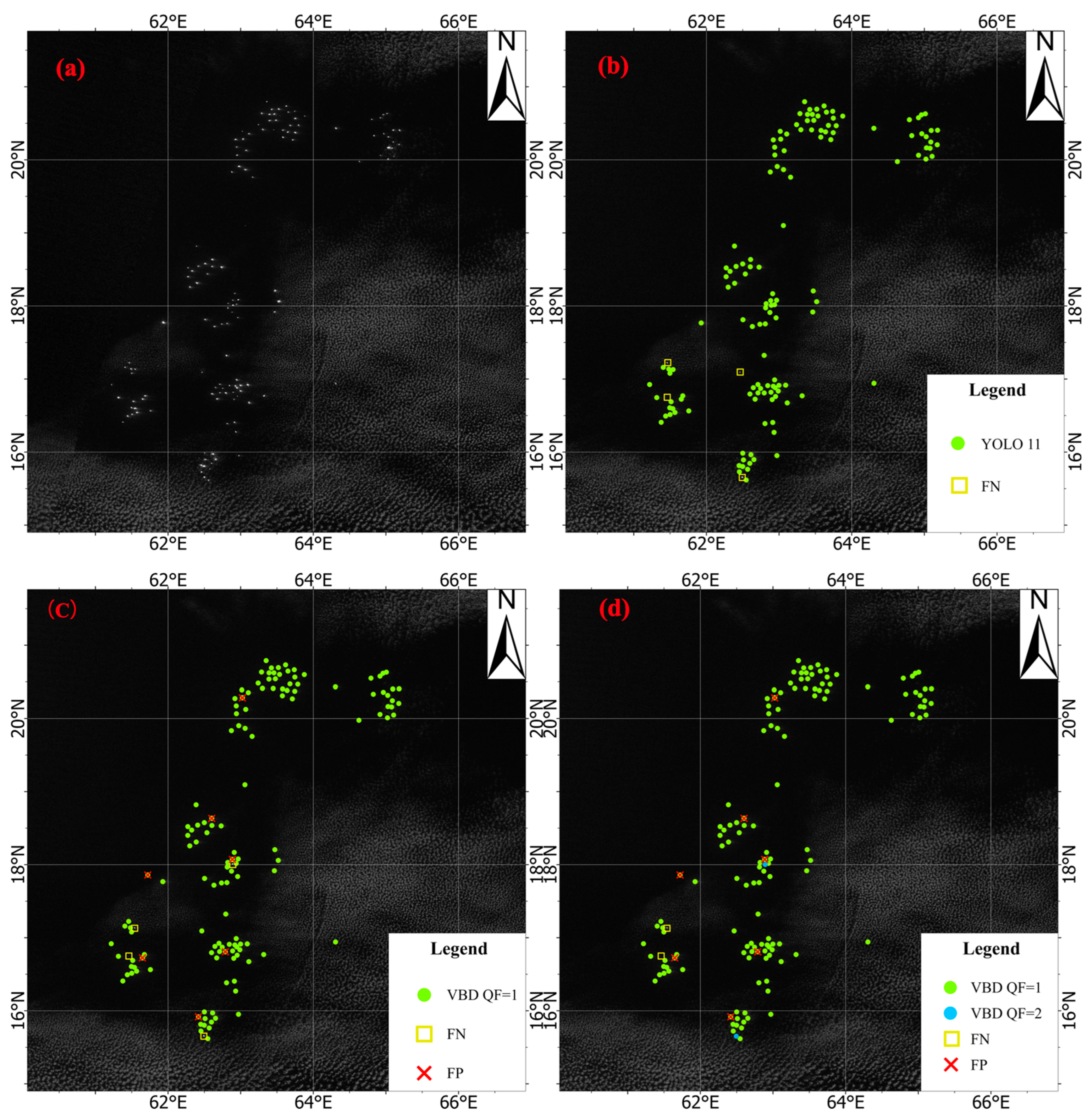
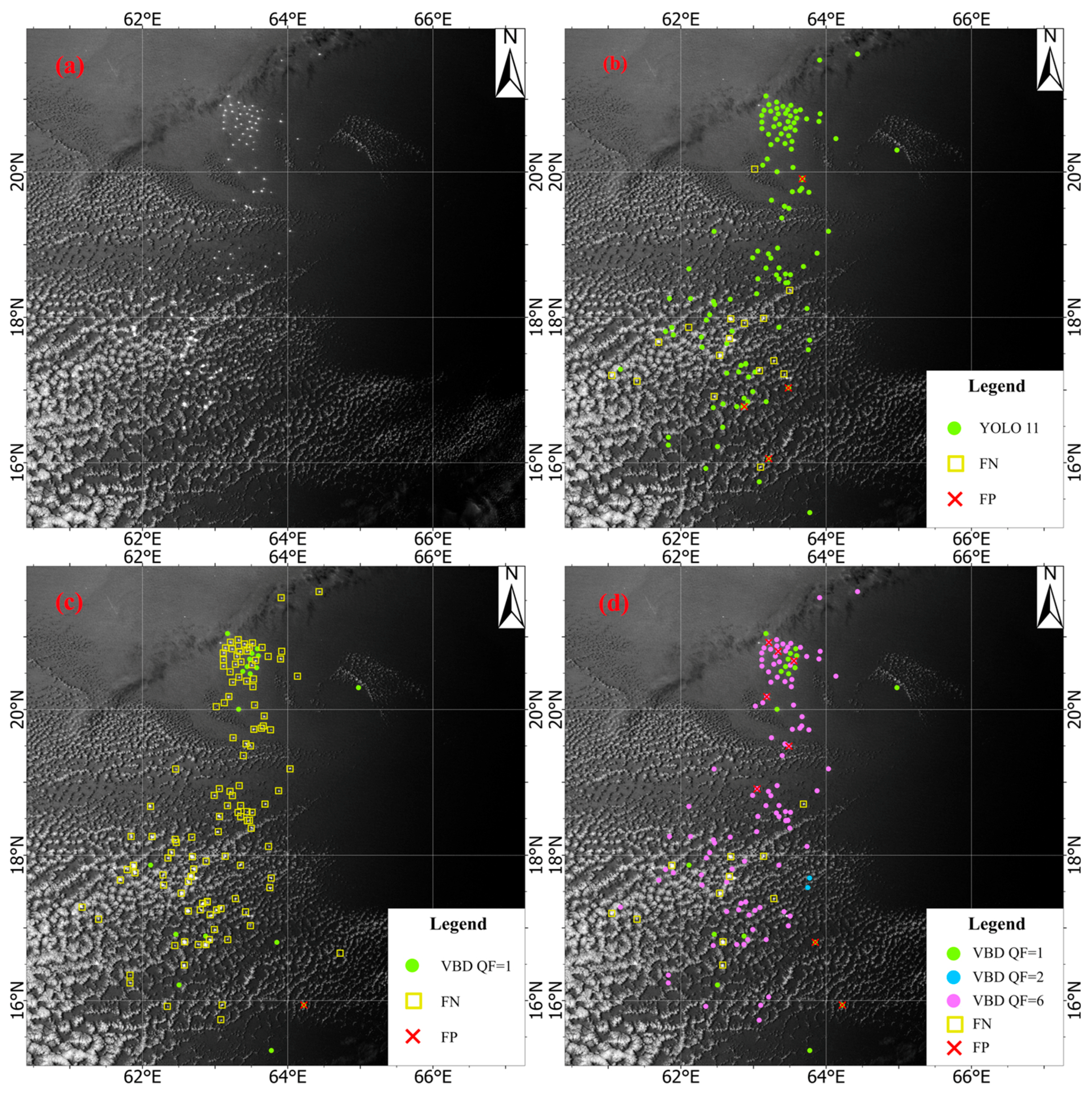
The comparison results between the YOLOv11 model and the VBD product under clear-sky and thin-cloud conditions are presented in Figure 3 and Figure 4, respectively. In the clear-sky scenario (22 December 2021), a total of 138 light-fishing vessels were confirmed (Figure 3a). The YOLOv11 algorithm (Figure 3b) successfully identified 134 targets with zero false alarms (i.e., false positives, FP = 0). In contrast, the standard VBD product (Quality Flag QF = 1, Figure 3c) identified 141 targets, which included seven false alarms. Although combining the QF = 1 and QF = 2 levels (Figure 3d) slightly increased the number of correct identifications to 136, the seven false alarms persisted. These results reveal that while the VBD product may have a marginally higher recall under ideal conditions, YOLOv11 demonstrates superior precision, which is critical for preventing the overestimation of fishing effort.

In the thin-cloud-cover scenario (16 December 2021), the advantages of the YOLOv11 framework were particularly pronounced. Out of 133 confirmed vessels (Figure 4a), YOLOv11 successfully identified 117 with high structural integrity (Figure 4b). Because cloud cover obstructed the sharp radiance peaks required by threshold-based discrimination methods, the standard QF = 1 VBD product (Figure 4c) performed poorly, missing 115 vessels. Even with the most comprehensive VBD configuration (encompassing QF = 1, 2, and 6; Figure 4d), eight false alarms and 11 missed detections still occurred.

3.2. Spatial Characteristics of Light-Fishing Activities

3.2.1. Spatiotemporal Distribution of Light-Fishing Activities

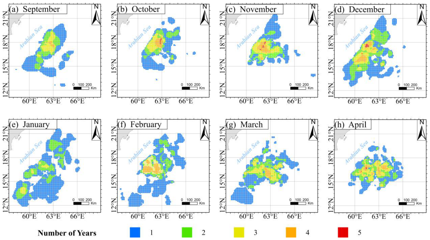
The spatiotemporal distribution of light-fishing activities (Figure 5) reveals a distinct seasonal “aggregation–diffusion–re-aggregation” pattern, with varying degrees of interannual spatial consistency.

From September to December, fishing activities are characterized by high spatial aggregation and predictability. In September, stable core FOAs (with a 4-year occurrence frequency) are primarily concentrated in the northeastern region (17.4–18.1° N, 62.5–63.1° E). This aggregation trend intensifies in October and November, with the maximum occurrence frequency reaching 5 years. During these peak months, the core clusters (17.4–18.1° N, 62.5–63.1° E) represent the most reliable FOAs, with as many as 135 grid cells maintaining a 4-year persistence. By December, although the maximum frequency remains at 5 years, the stable FOAs exhibit a slight westward shift (61.3–61.7° E), while maintaining a continuous presence within the central Arabian Sea basin.

Between January and February, a significant shift in spatial persistence occurs. In January, the FOAs disperse into three distinct clusters located near 14° N, 16° N, and 17° N, with the maximum occurrence frequency dropping to 3 years. In February, despite a broad spatial extent, stability begins to recover; a total of 185 grid cells between 16.0° N and 17.7° N demonstrate a 4-year persistence.

From March to April, the fleet’s operational range reaches its maximum spatial extent. In March, 351 grid cells show a 3-year persistence across a wide longitudinal span (59.7–65.5° E). By April, spatial stability reaches a second peak, with 126 grid cells exhibiting 4-year persistence and 366 cells maintaining 3-year persistence. These FOAs are primarily distributed between 14.4° N and 17.8° N, indicating a sustained and extensive re-aggregation of fishing effort prior to the monsoon-driven fishing moratorium. The high-frequency overlap (5 consecutive years) observed within the 16.7° N and 16.8° N zones further confirms this area as a core operational site consistently utilized by the light-fishing fleet during the late fishing season.

3.2.2. Distribution of the CoE for Light-Fishing Vessels

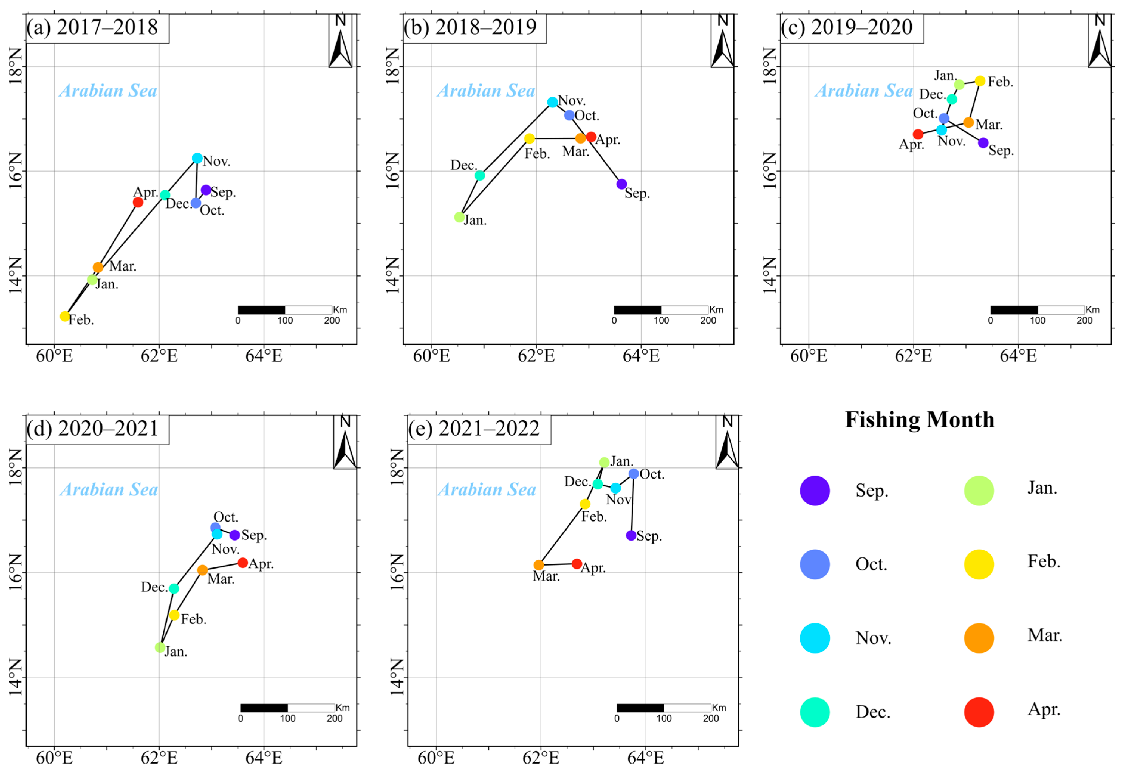
The distribution results for the CoE of light-fishing vessels (Figure 6) indicate that during four of the five analyzed fishing seasons (2017–2019 and 2020–2022), the CoE migration trajectories exhibited a counter-clockwise circulation pattern. These migrations typically originated in the northeast quadrant of the study area (September, located between 15.6° N and 16.7° N) and subsequently progressed in a southwestward direction during the northeast monsoon. In the 2017–2018 fishing season (Figure 6a), the CoE displayed a “W-shaped” trajectory, reaching its southernmost point (13.2° N, 60.2° E) in February before retreating to approximately 15.4° N in April. In contrast, the distribution for the 2021–2022 season was shifted northward as a whole, with the CoE remaining north of 16.1° N throughout the entire cycle and reaching its northernmost point (18.1° N) in January.

Departing from the aforementioned general trends, the 2019–2020 fishing season (Figure 6c) demonstrated a clockwise migration pattern. The CoE moved northwestward from September (16.5° N, 63.3° E) to January (17.7° N, 62.9° E). However, unlike the typical southwestward retreat observed in other years, the CoE in this particular season shifted northeastward during the mid-season before finally retreating southwestward as April approached (16.7° N, 62.1° E).

The magnitude of monthly CoE displacements also exhibited significant interannual variability. Large-scale spatial shifts occurred most frequently during the transition from the early to mid-season. For instance, the most substantial monthly displacement in the 2017–2018 season was recorded between December and the following January, whereas in the 2018–2019 and 2021–2022 seasons, the most significant shifts were observed from September to October and from February to March, respectively.

3.3. Environmental Impact Analysis of Fishing Operations

Variance Inflation Factor (VIF) analysis revealed that the VIF values for all 17 environmental variables were below 5, with the maximum value reaching only 4.56 (observed between Surface DO and DO50), indicating an absence of significant redundancy among the predictor variables.

To provide a comprehensive and rigorous assessment of model robustness and eliminate the contingency of single-data partitions, a multi-dimensional statistical validation was executed across 10 independent repetitions. The Random Forest model achieved an exceptional and highly stable overall mean validation accuracy of 96.87% ± 0.08%, with a remarkably narrow train-validation accuracy gap of only 3.13% ± 0.08%, empirically demonstrating that the model is well-calibrated and highly resistant to overfitting or underfitting. Furthermore, the ensemble evaluation yielded an average F1-score of 0.8367 ± 0.0038 and an Area Under the Receiver Operating Characteristic curve (AUC) of 0.9951 ± 0.0003. These well-aligned, high-precision diagnostic metrics collectively demonstrate the network’s high discriminative reliability, confirming its robust capability in characterizing the statistical relationships within light-fishing vessel distribution environments.

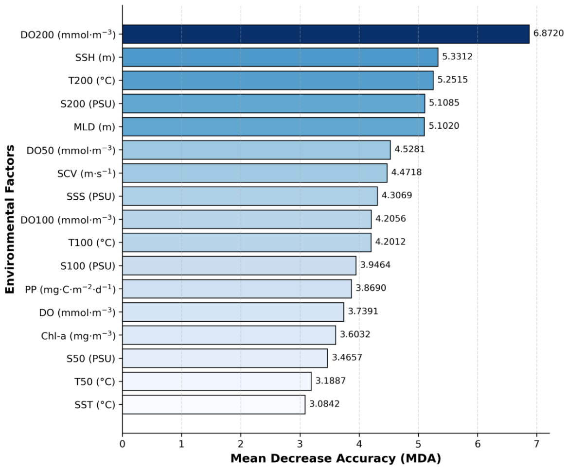
Variable importance assessment based on the Mean Decrease Accuracy (MDA) of the Random Forest model (Figure 7) indicated that among all environmental factors, dissolved oxygen at a depth of 200 m (DO200) provided the highest contribution to model prediction (MDA = 6.8720), followed by Sea Surface Height (SSH, 5.3312) and temperature at 200 m (T200, 5.2515). Conversely, Sea Surface Temperature (SST, 3.0842) exhibited the lowest contribution among the selected variables.

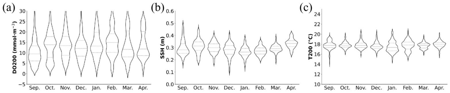
The relationships between monthly average DO200, SSH, and T200 and fishing vessel operations are illustrated in Figure 8. Overall, while the distributions of DO200, SSH, and T200 exhibited monthly variations, they remained relatively stable with minor fluctuations throughout the study period. In September, DO200 within the FOAs was primarily distributed between 6.1 and 13.4 mmol⋅m⁻³ (25th–75th percentiles), with a median of 9.5 mmol⋅m⁻³. The median peaked at 14.9 mmol⋅m⁻³ in February, and the 75th percentile reached 20.2 mmol⋅m⁻³ by April. Fishing vessel operations exhibited a pronounced spatial concentration within specific SSH corridors, predominantly occurring within the 0.24–0.36 m range. The median SSH peaked at 0.31 m in October, decreased to a minimum of 0.26 m in January, and subsequently rebounded to 0.33 m by April. T200 demonstrated high stability throughout the fishing season; during the observation cycle from September to the following April, the median T200 within the FOAs was strictly confined between 17.3 and 18.0 °C, while the core interquartile range (25th–75th percentiles) remained consistently stable between 17.2 and 18.4 °C.

4. Discussion

4.1. Analysis of Object Detection Model Performance and Data Advantages

The YOLOv11 architecture provides an efficient and robust technical framework for identifying light-fishing vessels in VIIRS/DNB imagery. Compared to previous object detection models, YOLOv5 maintains detail detection capabilities for small targets through its CSP backbone and PANet neck design, while YOLOv8 improves convergence and small-target fidelity via a decoupled head and anchor-free design [43]. Building upon these prior architectures, YOLOv11 enhances robust feature aggregation by introducing compact C3k2 bottlenecks and C2PSA attention modules, leading to superior small-target detection in medium-density scenarios and demonstrating strong applicability for VIIRS/DNB remote sensing monitoring.

Furthermore, the YOLOv11 model effectively bridges the performance gap of standard VBD products across different Quality Flags (QFs). Although VBD utilizes specialized modules to adaptively adjust detection thresholds based on lunar glint and specular reflection effects [44], YOLOv11 is capable of directly learning and mastering these complex features through its inherent feature extraction mechanism. This automated solution eliminates the tedious requirement for manual parameter tuning and ensures the consistency of vessel positioning data.

Compared to previous studies heavily reliant on the Automatic Identification System (AIS), this research utilizes deep learning technology to overcome the inherent limitations of AIS, such as discontinuous coverage in high seas and transponder shutdowns. The objective and continuous vessel activity records provided by YOLOv11 effectively compensate for the shortcomings of both AIS and standard VBD products. Such high-fidelity positioning data allows for a more detailed characterization of FOAs, laying the foundation for reconstructing high-precision spatial patterns of fishing effort.

4.2. Spatiotemporal Evolution Characteristics of Light-Fishing Activities

This study reveals a distinct seasonal “aggregation–diffusion–re-aggregation” dynamic pattern of light-fishing vessels in the Arabian Sea, which suggests a potential spatial alignment of the fleet with the seasonal monsoon-driven evolution of the marine environment. In autumn (September–December), as the southwest monsoon weakens, the Mixed Layer Depth (MLD) significantly shallows (<30 m), leaving abundant nutrients from summer upwelling unconsumed [45]. This stable, stratified shallow water column is hypothesized to provide a concentrated forage base for light-attracted pelagic species, offering a plausible ecological context that explains why the fleet forms highly aggregated core FOAs. During winter (January–February), the vigorous and dry-cold northeast monsoon triggers intense evaporative cooling and convective mixing, causing the MLD to surge beyond 70 m [46]. This hydrological transition may expand the vertical and horizontal habitats of target species, which could theoretically prompt the fleet to shift from ‘concentrated operations in core areas’ to ‘wide-ranging searches across regions,’ resulting in the observed discretized operational distribution. In spring (March–April), the monsoon transition causes the MLD to rapidly rise back to approximately 20 m, and the water column re-enters a stable stratified phase [46]. The anticipated re-aggregation of biological resources offers a reasonable explanation for why vessels converge once again toward the end of the fishing season.

Notably, this study observed an anomalous clockwise migration pattern of the CoE during the 2019–2020 fishing season, which closely coincides with the outbreak of an extreme positive Indian Ocean Dipole (pIOD) event. The 2019 pIOD was one of the strongest in nearly four decades, occurring superimposed with El Niño and an abnormally prolonged strong southwest monsoon that persisted until October [47]. Under the synergistic effect of multi-scale climate events, the heavy precipitation induced by the pIOD led to a significant freshening of Sea Surface Salinity (SSS) in the southeastern Arabian Sea and triggered a drastic adjustment of surface current fields [47]. This cross-scale marine environmental anomaly likely reshaped conventional habitat patterns and may have served as a major contributing factor associated with the observed inversion of the CoE trajectory.

In summary, while the seasonality of the mixed layer in the Arabian Sea and extreme climate events offer a highly cohesive conceptual framework for understanding shifts in FOAs and centers of gravity, these linkages remain diagnostic hypotheses rather than quantitatively modeled relationships within the scope of this study. Future research should further integrate in situ current dynamics, mesoscale eddies, and biological catch data to quantitatively validate and more comprehensively reveal the empirical response of fishing effort to multi-scale environmental changes in this region.

4.3. Multi-Dimensional Habitat Preferences and Key Driver Analysis

Previous modeling efforts have largely operated under the assumption that pelagic habitats are primarily associated with sea surface environments, identifying SST, SSH, SSS, and Chl-a as the dominant indicators [17]. However, this assumption—derived primarily from research in the Northwest Pacific or the South China Sea—may not be fully transferable to the unique oceanographic conditions of the Arabian Sea. Our MDA importance assessment reveals that dissolved oxygen at 200 m (DO200) and temperature at 200 m (T200) contribute significantly more to the spatial characterization of FOAs than surface factors such as SST. This suggests that subsurface vertical hydrological structures may act as critical environmental constraints modulating the spatial distribution of S. oualaniensis. While previous studies noted the influence of dissolved oxygen [18], they focused predominantly on the surface or shallow layers. Incorporating these subsurface parameters is therefore highly beneficial for achieving a more balanced predictive mapping of the Arabian Sea’s light-fishing industry. Nevertheless, it is critical to note that the feature importance derived from the Random Forest model establishes statistical associations rather than direct mechanistic causation. The high explanatory power of DO200 and T200 likely reflects indirect ecological linkages, and further interdisciplinary research combining fishery biological data is required to fully elucidate the underlying causal mechanisms.

Compared to studies based on limited exploratory surveys [16] or commercial logbooks [14,15,17,18,19,20], this research utilizes high-frequency vessel positioning data covering the entire basin across five fishing seasons. This approach overcomes traditional limitations such as coarse station density, short survey durations, and narrow spatial coverage, ensuring spatiotemporal consistency between environmental factors and fishing intensity while effectively reducing statistical bias.

Furthermore, while previous research frequently employed Catch Per Unit Effort (CPUE) as a metric to characterize the center of FOAs, this study focuses on the dynamic evolution of fishing effort (spatial distribution) itself. CPUE primarily reflects local biological abundance, whereas the spatial pattern of fishing effort may be more constrained by macro-physical habitat boundaries. This shift in evaluation metrics may partially explain why the importance ranking of environmental factors in this study diverges from previous conclusions.

4.4. Limitations and Future Perspectives

Several limitations remain in this study, which point to clear directions for future research.

First, regarding the temporal scale, although this study captures a highly distinct spatial anomaly during the 2019–2020 fishing season coinciding with an extreme pIOD event, the five-season time series remains insufficient to conduct direct, rigorous correlation analyses with quantitative climate indices (such as the Dipole Mode Index). Consequently, the proposed linkage between large-scale climate variability and CoE shifts remains primarily descriptive at this stage. Future work requires the continuous accumulation of decadal-scale remote sensing observations to statistically quantify and verify the universal impact of pIOD events on CoE trajectory inversions through long-sequence empirical modeling.

Second, in terms of data dimensions, current research focuses primarily on physical environmental factors and has yet to deeply integrate biological information (e.g., body size, sexual maturity, and age). Future research should further integrate in situ biological sampling data with multi-scale physical processes—such as upwelling and mesoscale eddies—to provide a more robust scientific foundation for the sustainable utilization and precision forecasting of high-seas resources in the Arabian Sea.

Third, regarding ecological interpretation and operational data constraints, it must be cautiously noted that this study primarily evaluates fleet operational distributions derived from nighttime light vessel density, rather than direct squid abundance or true habitat occupancy. This reliance on fishing effort as a behavioral proxy introduces non-environmental confounders—including socio-economic vectors (e.g., fuel costs and logistical distance to ports) and geopolitical or regulatory influences (e.g., Exclusive Economic Zone boundaries and maritime security corridors)—that may decouple fishing intensity from pure environmental drivers. Furthermore, because the model captures oceanographic profiles unique to the Arabian Sea (such as severe subsurface hypoxia), its direct geographic generalization to other basins remains limited without localized recalibration. Independent external validation is also structurally constrained by the extreme scarcity and confidentiality of public high-seas commercial logbooks. Therefore, future iterative frameworks must integrate socio-economic indicators and cross-regional datasets from other global fishing grounds—such as the Southwest Atlantic and Northwest Pacific squid jigging sectors—to decouple non-biological drivers, evaluate out-of-sample transferability, and support standardized global high-seas fisheries governance.

5. Conclusions

This study elucidates the spatiotemporal dynamics of light-fishing FOAs in the Arabian Sea by integrating the YOLOv11 framework with multi-parameter marine environmental analysis. The key findings are as follows:

(1)

The YOLOv11 model exhibited superior performance in light-fishing vessel detection, achieving an mAP of 0.969 and an F1-score of 0.960. This automated approach effectively addresses the coverage gaps inherent in AIS data within high-sea regions, providing robust technical support for the construction of high-fidelity fishing effort datasets.

(2)

The operational distribution of the fleet follows a distinct seasonal ‘aggregation–diffusion–re-aggregation’ pattern coinciding with the seasonal progression of the monsoon cycle. The anomalous reversal of the CoE trajectory observed during the 2019–2020 fishing season aligns closely with the outbreak of a strong positive Indian Ocean Dipole (pIOD) event, suggesting a potential behavioral adjustment of the fleet to large-scale climate anomalies. However, due to the five-season observation span, these macro-climate linkages remain exploratory, and an extended time series is required to systematically confirm long-term periodic impacts.

(3)

The study highlights a significant correlation between fishing operation preferences and subsurface environmental parameters (T200, D200), suggesting that subsurface hydrological structures exhibit a strong statistical association with the spatial characterization of operational environments. These findings provide a preliminary scientific basis for the sustainable management and resource forecasting of fisheries in the Northwest Indian Ocean.

References

1. Yang, S.; Yu, L.; Jiang, K.; Fan, X.; Wan, L.; Fan, W.; Zhang, H. Spatiotemporal Analysis of Light Purse Seine Fishing Vessel Operations in the Arabian High Seas Based on Automatic Identification System Data. Appl. Sci. 2024, 14, 10692. [Google Scholar] [CrossRef]
2. Nguyen, K.Q.; Winger, P.D. Artificial Light in Commercial Industrialized Fishing Applications: A Review. Rev. Fish. Sci. Aquac. 2018, 27, 106–126. [Google Scholar] [CrossRef]
3. Madhupratap, M.; Kumar, S.P.; Bhattathiri, P.; Kumar, M.D.; Raghukumar, S.; Nair, K.; Ramaiah, N. Mechanism of the biological response to winter cooling in the northeastern Arabian Sea. Nature 1996, 384, 549–552. [Google Scholar] [CrossRef]
4. Quan, L. Evaluation and Management Countermeasures of Sustainable Utilization of Fishery Resources in the Indian Ocean. Ph.D. Thesis, Shanghai Ocean University, Shanghai, China, 2022. [Google Scholar]
5. Zuev, G.; Nigmatullin, C.; Chesalin, M.; Nesis, K. Main results of long-term worldwide studies on tropical nektonic oceanic squids genus Sthenoteuthis: An overview of the Soviet investigations. Bull. Mar. Sci. 2002, 71, 1019–1060. [Google Scholar]
6. Chen, X.J.; Qian, W.G. Study on the resource density distribution of Symlectoteuthis oualaniensis in the northwestern Indian Ocean. J. Shanghai Ocean. Univ. 2004, 3, 218–223. [Google Scholar]
7. Shao, F.; Chen, X.J. Relationship between fishing ground of Symlectoteuthis oualaniensis and sea surface height in the northwest Indian ocean. Mar. Sci. 2008, 32, 88–92. [Google Scholar]
8. Chen, X.J.; Ye, X.C. Preliminary study on the relationship between fishing ground of Symlectoteuthis oualaniensis and environmental factors in northwestern Indian Ocean. J. Shanghai Fish. Univ. 2005, 14, 55–60. [Google Scholar]
9. Chen, X.J.; Qian, W.G.; Tian, S.Q. Resource Density and Distributions of Symlectoteuthis oualaniensis in Open Seas of Northern Arabian Sea. Adv. Mar. Sci. 2006, 3, 360–364. [Google Scholar]
10. Chen, X.J.; Shao, F. Study on the Resource Characteristics of Symlectoteuthis oualaniensis and Their Relationships with the Sea Conditions in the High Sea of the Northwestern Indian Ocean. Period. Ocean Univ. China 2006, 36, 611–616. [Google Scholar] [CrossRef]
11. Lin, D.M.; Chen, X.J. Fishing Ground Distribution of Symplectoteuthis ouslsniensis and Its Relations to SST in the Northwestern Indian Ocean. Adv. Mar. Sci. 2006, 24, 546–551. [Google Scholar]
12. Tian, S.Q.; Chen, X.J.; Yang, X.M. Study on the fishing ground distribution of Symlectoteuthis oualaniensis and its relationship with the environmental factors in the high sea of the Northern Arabian Sea. Trans. Oceanol. Limnol. 2006, 1, 51–57. [Google Scholar] [CrossRef]
13. Yang, X.M.; Chen, X.J.; Zhou, Y.Q.; Tian, S.Q. A marine remote sensing-based preliminary analysis on the fishing ground of purple flying squid Sthenoteuthis oualaniensis in the northwest Indian Ocean. J. Fish. China 2006, 5, 669–675. [Google Scholar]
14. Yang, S.L.; Fan, X.M.; Wu, Y.M.; Zhou, W.F.; Wang, F.; Wu, Z.; Zhang, B.B.; Fan, W. The relationship between the fishing ground of mackerel (Scomber australasicus) in Arabian Sea and the environment based on GAM model. Chin. J. Ecol. 2019, 38, 2466–2470. [Google Scholar] [CrossRef]
15. Yang, S.L.; Fan, X.M.; Tang, F.H.; Tianfei, C.; Fan, W. Relationship between spatial-temporal distribution of Scomber australasicus and environmental factors in the Arabian Sea. J. Trop. Oceanogr. 2019, 38, 91–100. [Google Scholar]
16. Xiao, G.; Xu, B.; Zhang, H.; Tang, F.H.; Chen, F.; Zhu, W.B. A study on spatial-temporal distribution and marine environmental elements of Symplectoteuthis oualaniensis fishing grounds in outer sea of Arabian Sea. South China Fish. Sci. 2022, 18, 10–19. [Google Scholar]
17. Wen, L.H.; Zhang, H.; Fang, Z.; Chen, X.J. Preliminary standardization of Sthenoteuthis oualaniensis in northern Indian Ocean. Trans. Oceanol. Limnol. 2022, 44, 89–97. [Google Scholar] [CrossRef]
18. Han, H.; Yang, C.; Zhang, H.; Fang, Z.; Jiang, B.; Su, B.; Sui, J.; Yan, Y.; Xiang, D. Environment variables affect CPUE and spatial distribution of fishing grounds on the light falling gear fishery in the Northwest Indian Ocean at different time scales. Front. Mar. Sci. 2022, 9, 1455. [Google Scholar] [CrossRef]
19. Yang, S.L.; Fan, X.M.; Zhang, B.B.; Zhang, H.; Zhang, S.M.; Cui, X.S.; Fan, W. Spatial-temporal Distribution of Purse Seine in Arabian Sea and Its Relationship With Sea Surface Environmental Factors. J. Agric. Sci. Technol. 2019, 21, 149–158. [Google Scholar] [CrossRef]
20. Wen, L.H.; Zhang, H.; Fang, Z.; Chen, X.J. Spatial and temporal distribution of fishing ground of Sthenoteuthis oualaniensis in northern Indian Ocean with different fishing methods. J. Shanghai Ocean. Univ. 2021, 30, 1079–1089. [Google Scholar]
21. Croft, T.A. Nighttime images of the earth from space. Sci. Am. 1978, 239, 86–101. [Google Scholar] [CrossRef]
22. Cho, K.; Ito, R.; Shimoda, H.; Sakata, T. Technical note and cover Fishing fleet lights and sea surface temperature distribution observed by DMSP/OLS sensor. Int. J. Remote Sens. 1999, 20, 3–9. [Google Scholar] [CrossRef]
23. Rodhouse, P.; Elvidge, C.; Trathan, P. Remote Sensing of the Global Light-Fishing Fleet: An Analysis of Interactions with Oceanography, Other Fisheries and Predators; Academic Press: London, UK, 2001. [Google Scholar]
24. Waluda, C.M.; Trathan, P.N.; Elvidge, C.D.; Hobson, V.R.; Rodhouse, P.G. Throwing light on straddling stocks of Illex argentinus: Assessing fishing intensity with satellite imagery. Can. J. Fish. Aquat. Sci. 2002, 59, 592–596. [Google Scholar] [CrossRef]
25. Ito, R.; Cho, K.; Shimoda, H.; Sakata, T.; Saitoh, S.-I. The impact of Japan/South Korea Fishery Agreement observed in the light-fishing fleet distribution captured by night time DMSP/OLS images. J. Jpn. Soc. Photogramm. Remote Sens. 2002, 41, 39–46. [Google Scholar][Green Version]
26. Kiyofuji, H.; Saitoh, S.-I. Use of nighttime visible images to detect Japanese common squid Todarodes pacificus fishing areas and potential migration routes in the Sea of Japan. Mar. Ecol. Prog. Ser. 2004, 276, 173–186. [Google Scholar] [CrossRef]
27. Semedi, B.; Saitoh, S.-i.; Saitoh, K.; Yoneta, K. Application of multi-sensor satellite remote sensing for determining distribution and movement of Pacific saury Cololabis saira. Fish. Sci. 2002, 68, 1781–1784. [Google Scholar] [CrossRef][Green Version]
28. Waluda, C. Quantifying light-fishing for Dosidicus gigas in the eastern Pacific using satellite remote sensing. Remote Sens. Environ. 2004, 91, 129–133. [Google Scholar] [CrossRef]
29. Waluda, C.M.; Griffiths, H.J.; Rodhouse, P.G. Remotely sensed spatial dynamics of the Illex argentinus fishery, Southwest Atlantic. Fish. Res. 2008, 91, 196–202. [Google Scholar] [CrossRef]
30. Cheng, T.; Zhou, W.; Xu, H.; Fan, W. Estimation of fishing vessel numbers close to the terminator in the pacific northwest using OLS/DMSP data. In Proceedings of the International Conference on Geo-Informatics in Resource Management and Sustainable Ecosystem, Hong Kong, China, 18–20 November 2016; pp. 321–327. [Google Scholar]
31. Elvidge, C.D.; Zhizhin, M.; Baugh, K.; Hsu, F.C. Automatic Boat Identification System for VIIRS Low Light Imaging Data. Remote Sens. 2015, 7, 3020–3036. [Google Scholar] [CrossRef]
32. Kim, E.; Kim, S.-W.; Jung, H.C.; Ryu, J.-H. Moon phase based threshold determination for VIIRS boat detection. Korean J. Remote Sens. 2021, 37, 69–84. [Google Scholar]
33. Li, X.; Xu, Q.; Wang, H.; Jiang, H.; Yin, X.; Mu, S.; Li, X.; Su, H.; Wang, A.; Yang, Y.; et al. AI in Satellite Remote Sensing of the Ocean. Proc. IEEE 2026, 1–34. [Google Scholar] [CrossRef]
34. Zuo, G.; Zhou, J.; Meng, Y.; Zhang, T.; Long, Z. Night-Time Vessel Detection Based on Enhanced Dense Nested Attention Network. Remote Sens. 2024, 16, 1038. [Google Scholar] [CrossRef]
35. Shao, J.; Yang, Q.; Luo, C.; Li, R.; Zhou, Y.; Zhang, F. Vessel detection from nighttime remote sensing imagery based on deep learning. IEEE J. Sel. Top. Appl. Earth Obs. Remote Sens. 2021, 14, 12536–12544. [Google Scholar] [CrossRef]
36. Hu, H.; Zhou, W.; Jiang, B.; Zhang, J.; Cheng, T. Exploring deep learning techniques for the extraction of lit fishing vessels from Luojia1-01. Ecol. Indic. 2024, 159, 111682. [Google Scholar] [CrossRef]
37. Li, J.; Li, J.; Zhang, K.; Li, X.; Chen, Z. Enhanced Fishing Monitoring in the Central-Eastern North Pacific Using Deep Learning with Nightly Remote Sensing. Remote Sens. 2024, 16, 4312. [Google Scholar] [CrossRef]
38. Shankar, D.; Vinayachandran, P.; Unnikrishnan, A. The monsoon currents in the north Indian Ocean. Prog. Oceanogr. 2002, 52, 63–120. [Google Scholar] [CrossRef]
39. Wan, L.; Cheng, T.; Fan, W.; Shi, Y.; Zhang, H.; Zhang, S.; Yu, L.; Dai, Y.; Yang, S. Spatial information extraction of fishing grounds for light purse seine vessels in the Northwest Pacific Ocean based on AIS data. Heliyon 2024, 10, e28953. [Google Scholar] [CrossRef]
40. Chen, R.; Wu, X.; Liu, B.; Wang, Y.; Gao, Z. Mapping coastal fishing grounds and assessing the effectiveness of fishery regulation measures with AIS data: A case study of the sea area around the Bohai Strait, China. Ocean. Coast. Manag. 2022, 223, 106136. [Google Scholar] [CrossRef]
41. Menard, S. Applied Logistic Regression Analysis; Sage: Thousand Oaks, CA, USA, 2002. [Google Scholar]
42. Bui, D.T.; Lofman, O.; Revhaug, I.; Dick, O. Landslide susceptibility analysis in the Hoa Binh province of Vietnam using statistical index and logistic regression. Nat. Hazards 2011, 59, 1413–1444. [Google Scholar] [CrossRef]
43. Sapkota, R.; Karkee, M. Ultralytics YOLO evolution: An overview of YOLO26, YOLO11, YOLOv8 and YOLOv5 object detectors for computer vision and pattern recognition. arXiv 2025, arXiv:2510.09653. [Google Scholar]
44. Elvidge, C.D.; Ghosh, T.; Chatterjee, N.; Zhizhin, M.; Sutton, P.C.; Bazilian, M. A comprehensive global mapping of offshore lighting. Earth Syst. Sci. Data 2025, 17, 579–594. [Google Scholar] [CrossRef]
45. Shi, W.; Morrison, J.M.; Böhm, E.; Manghnani, V. The Oman upwelling zone during 1993, 1994 and 1995. Deep Sea Res. Part II Top. Stud. Oceanogr. 2000, 47, 1227–1247. [Google Scholar]
46. Ma, J.F. The Responses and Feedbacks of the Chlorophyll to Upwelling of the Indian Ocean. Ph.D. Thesis, University of Chinese Academy of Sciences, Beijing, China, 2013. [Google Scholar]
47. Nyadjro, E.S. Impacts of the 2019 strong IOD and monsoon events on Indian Ocean sea surface salinity. Remote Sens. Earth Syst. Sci. 2021, 4, 158–171. [Google Scholar] [CrossRef]
Figure 1. Methodological framework for the analysis of spatiotemporal dynamics and environmental drivers of light-fishing vessels in the Arabian Sea.
Fishes 11 00324 g001
Figure 2. Detailed architecture of the YOLOv11-based vessel detection pipeline, integrating offline model training and online geospatial inference.
Fishes 11 00324 g002
Figure 3. Comparison of maritime vessel detection capabilities under clear sky conditions in the Arabian Sea (observed on 22 December 2021): (a) original VIIRS DNB radiance image showcasing active light-fishing vessels against a low-noise background; (b) target extraction results achieved by the proposed YOLOv11 model; (c) official VBD product results restricted strictly to detections with a strong quality flag (QF = 1); (d) integrated VBD product results incorporating both strong and weak quality flags (QF = 1 and QF = 2).
Fishes 11 00324 g003
Figure 4. Comparison of maritime vessel detection capabilities under thin cloud cover in the Arabian Sea (observed on 16 December 2021): (a) original VIIRS DNB radiance image; (b) spatial extraction results of the trained YOLOv11 model; (c) standard VBD product results with a strong quality flag filter (QF = 1); (d) comprehensive VBD product results integrated across multiple detection thresholds, including strong quality flag, weak quality flag, and lunar glint detections (QF = 1, QF = 2, and QF = 6).
Fishes 11 00324 g004
Figure 5. Monthly spatiotemporal persistence and occurrence frequency of FOAs in the Arabian Sea from 2017 to 2022. The color scale represents the number of years (out of five fishing seasons) each 0.1° × 0.1° grid cell was identified as FOAs.
Fishes 11 00324 g005
Figure 6. Inter-annual and seasonal migration trajectories of the CoE in the central Arabian Sea from 2017 to 2022. Panels (ae) represent five consecutive fishing seasons.
Fishes 11 00324 g006
Figure 7. Relative importance of environmental factors for identifying the habitat preferences of light-fishing vessels based on Mean Decrease Accuracy (MDA).
Fishes 11 00324 g007
Figure 8. Monthly environmental envelopes of (a) DO200, (b) SHH, and (c) T200 within the FOAs in the Arabian Sea (2017–2022). Each violin plot shows the frequency distribution and statistical quartiles (median and IQR) of the respective environmental factor for each month of the fishing season.
Fishes 11 00324 g008