Projected Impacts of Extreme Drought on Tilapia Aquaculture in Guangdong, China, Under SSP Scenarios: Climate-Yields Modeling Approach Using Loss Function

Abstract

Global warming presents urgent challenges for tilapia aquaculture. This study introduces a tailored loss function to assess long-term impacts under extreme drought, using historical drought data in China as a baseline. The TaiESM1 climate model within the CMIP6 framework is applied to project future conditions under SSP245, SSP370, and SSP585 scenarios, focusing on Guangdong Province (2024–2100). The results indicate a general decline in the frequency of extreme droughts across all scenarios. Under SSP245, technological advancements combined with reduced drought risk may boost yields of tilapia aquaculture of Guangdong to 2.369–2.418 million tons by 2100. In SSP370 and SSP585, while humidity increases, drought risk reduction is less pronounced, resulting in marginally lower yields (2.285–2.408 and 2.300–2.416 million tons, respectively). When a unified loss parameter is applied, projected yields exhibit a U-shaped trend across all SSP scenarios, reaching a minimum under SSP370 in the mid-century period before recovering toward the end of the century, driven by scenario-dependent marginal responses of production to changes in extreme drought risk, highlighting the nonlinearity of climate impacts driven by complex climatic factors and socioeconomic interactions. These findings are subject to uncertainties associated with the use of a single climate model and the simplified representation of drought impacts in the loss-function framework.

1. Introduction

Amid escalating global climate change, the rising frequency and intensity of extreme weather events have become major threats to sectors that depend on natural ecosystems, particularly agriculture and aquaculture [1]. Within this context, freshwater aquaculture, especially tilapia farming, which is widely practiced in tropical and subtropical regions, is facing mounting ecological and economic pressures. Events such as heatwaves, flash floods, prolonged droughts, and cold spells can disrupt aquatic environments, leading to higher rates of disease, increased fish escapes, and elevated mortality. These disruptions not only undermine production efficiency but also pose critical risks to the livelihoods of aquaculture-reliant communities [2,3].

Given its ecological adaptability and global significance, tilapia has emerged as a focal species in climate change-related aquaculture research. A growing body of interdisciplinary studies has investigated how extreme climate conditions affect tilapia farming, offering insights that span environmental variability, physiological resilience, genetic adaptability, and policy innovation. These studies collectively highlight the multifaceted vulnerability of tilapia aquaculture systems in a rapidly changing climate.

At the ecosystem level, empirical evidence underscores how environmental extremes can directly disrupt farm operations. For instance, Pimolrat et al. [4] documented that high-altitude pond farms in northern Thailand experienced increased tilapia mortality during droughts and cold spells, forcing farmers to shorten or suspend production cycles as a risk management strategy. Complementing this, Ribeiro et al. [5] demonstrated through laboratory experiments that the combined exposure to high temperatures and copper contamination caused severe tissue damage and acute stress behaviors in tilapia. These findings suggest that climate-induced temperature extremes may intensify the harmful effects of existing pollutants, creating compounding environmental stressors.

Beyond physical habitat impacts, disease dynamics present another critical dimension of vulnerability. In a comprehensive ten-year epidemiological study, Liao et al. [6] found strong correlations between Streptococcus outbreaks in tilapia and climatic variables such as temperature, ultraviolet radiation, and precipitation in Taiwan. Notably, disease incidence spiked when water temperatures exceeded 27 °C, particularly under conditions of low atmospheric pressure. This highlights the complex, nonlinear interplay between climatic stress and pathogen behavior, with serious implications for health management in aquaculture systems.

Meanwhile, research on physiological and genetic adaptation has provided deeper insights into how tilapia responds to thermal stress. Wang et al. [7] observed that prolonged exposure to elevated temperatures altered energy metabolism pathways in tropical tilapia strains. However, this physiological adaptation came at the cost of reduced cold tolerance, suggesting a potential evolutionary trade-off. Similarly, wild strains from the Oti River outperformed commercial strains under high-temperature and hypoxic conditions, pointing to the untapped potential of local genetic resources in breeding climate-resilient brood stock.

At the molecular scale, innovations in genomic tools are beginning to inform future adaptation strategies. Mehta et al. [8], for instance, used ATAC-seq to identify regulatory elements in tilapia gill tissues related to osmoregulation and salinity tolerance, offering a valuable foundation for precision breeding in the face of environmental stress.

While biological adaptations are crucial, they must be complemented by innovations in farming systems and governance. In this regard, several studies have proposed integrated solutions that address both ecological and socioeconomic challenges. Tran et al. [9] evaluated an integrated multi-trophic aquaculture (IMTA) system combining tilapia, shrimp, and seaweed, which demonstrated improved productivity and ecosystem stability in Vietnam. On the post-harvest side, Chua [10] introduced a vacuum-sealing technique for tilapia “tocino” which extended shelf life up to one year, a practical intervention for coping with storage challenges during hot seasons. At the policy level, Uppanunchai et al. [11] assessed Thai aquaculture regulations and identified gaps in climate adaptation planning. While zoning and disaster relief provisions offer partial coverage, the absence of a comprehensive, tilapia-specific climate strategy remains a critical shortcoming.

Despite extensive research on climate impacts, existing studies largely focus on short-term responses and lack a mechanistic and quantitative assessment of how changes in extreme drought risk affect aquaculture production through biological pathways, particularly under long-term climate scenarios at regional scales.

More broadly, loss-function-based approaches have been widely used in agricultural and climate impact research to characterize how environmental stress translates into production losses. These approaches can be broadly grouped into two categories: empirical approaches that directly relate climate variables or hazard indicators to yield or output losses, and process-based approaches that represent the biophysical mechanisms through which environmental stress affects plant growth, development, and ultimately production outcomes [12,13,14,15]. However, such approaches have rarely been applied in aquaculture and fisheries. In particular, few studies integrate these mechanisms into a production framework that connects biological responses, such as juvenile survival, with economic outcomes.

To address this research gap, we adopt a loss-function-based approach embedded within a production framework, linking drought-induced changes in juvenile survival to yield growth and overall aquaculture output. We hypothesize that changes in extreme drought risk influence tilapia aquaculture primarily through their effects on juvenile survival, thereby shaping production outcomes. We further expect that this relationship is nonlinear across SSP scenarios, reflecting differences in the marginal impacts of drought risk under varying climate regimes. In addition, technological progress is hypothesized to play a dominant moderating role, offsetting potential losses from drought variability and driving long-term yield growth.

The study offers three core contributions. First, we introduce an innovative extreme drought risk factor that links drought severity to the survival and growth rates of tilapia fry. This factor is integrated into a linear model that quantifies the relationship between yield growth and changes in drought risk, providing a novel framework for forecasting production under variable climate conditions. Second, we incorporate future climate projections using the TaiESM1 model from CMIP6 and evaluate outcomes under three Shared Socioeconomic Pathways: SSP245, SSP370, and SSP585. Third, the analysis explicitly considers the moderating role of technological progress, which has often been overlooked in previous studies. This perspective enhances the practical relevance of our findings for policy and planning.

The remainder of the paper is structured as follows: Section 2 presents the methodology and data sources, including the development of the loss function for yield growth of tilapia aquaculture. Section 3 details the empirical results, including model validation and scenario-based projections of yield growth and yields. Section 4 concludes the study with key findings and discussion.

2. Method and Data

2.1. Extreme Drought-Yield Model of Tilapia

Biological impacts of extreme drought are incorporated into the economic model through their effects on juvenile survival, which determines effective stock input. This representation follows established approaches that integrate environmental stress into production frameworks via changes in effective inputs or productivity [16,17]. Thus, climate-induced mortality is captured as a reduction in effective capital within a CES production framework. The CES framework is widely used in economic and agricultural production analysis because it explicitly captures input substitutability while preserving analytical tractability. The original CES specification was developed precisely to represent substitution among production factors, and it remains one of the most frequently employed production functions in applied economic analysis [18,19,20]. This feature is also suitable for tilapia aquaculture systems. In aquaculture production, key inputs such as juvenile stock, labor, and aquaculture area are not perfectly fixed, but can be adjusted within practical limits under cost-minimizing behavior. More broadly, fisheries and aquaculture economics have long relied on production and bioeconomic modeling frameworks to analyze input use, productivity, and management decisions, which supports the extension of a CES-type production structure to this context [21]. In this study, the CES framework further provides a tractable way to incorporate drought-induced changes in juvenile survival into the economic production system.

This framework adopts a mechanism-isolation approach, focusing on the marginal effect of extreme drought on oxygen availability and juvenile survival as the primary transmission pathway to production outcomes. Similar approaches are widely used in the literature to incorporate environmental stress into economic production frameworks through changes in effective inputs or productivity [16,17]. Other interacting processes, including water quality dynamics, physiological stress responses, and disease, are not modeled explicitly but are implicitly captured within the survival-based representation. This simplification enables a clearer identification of the drought–production linkage within a consistent economic framework.

This study hypothesizes that extreme drought exerts its primary impact on tilapia yield by disrupting the growth and survival of juvenile fish [22,23]. Water shortages caused by drought conditions lower dissolved oxygen concentrations within fixed aquaculture areas, thereby increasing mortality rates among juvenile tilapia and ultimately reducing total production output [24].

In this context, we assume that tilapia producers in Guangdong Province operate under a cost-minimization objective for a given target yield. The production process is represented by a Constant Elasticity of Substitution (CES) production function, which is specified as follows:

$$Q=A{({\alpha }_1{K}^{-\rho }+{\alpha }_2{L}^{-\rho }+{\alpha }_{3}Q{A}^{-\rho })}^{-{\displaystyle \frac{1}{\rho }}}$$

(1)

$$Q>0,K>0,L>0,QA>0$$

(2)

$${\alpha }_1+{\alpha }_2+{\alpha }_3=1$$

(3)

$$0<-\rho <1$$

(4)

Equation (1) defines the CES production function, which describes how total output is generated from multiple inputs under a constant elasticity of substitution. Equations (2)–(4) represent the corresponding input demand or transformation relationships derived under cost-minimizing behavior. This specification follows the standard CES production function originally developed by Arrow et al. (1961) [18] and widely applied in economic analysis.

In Equations (1)–(3), Q denotes total tilapia output in Guangdong Province; K represents the number of juvenile tilapia stocked (i.e., biological capital input); L denotes the quantity of specialized aquaculture labor; and QA refers to the aquaculture area dedicated to tilapia farming. The parameters α₁, α₂, and α₃ are input share coefficients associated with each production factor, satisfying α₁ + α₂ + α₃ = 1. The parameter ρ governs the substitution structure of the CES function, with −1 < ρ < 0, implying a positive but limited degree of substitutability among inputs. The corresponding elasticity of substitution is given by σ = 1/(1 + ρ), indicating that inputs can be substituted, but not perfectly.

Empirical studies have shown that fish growth is highly sensitive to extreme drought events. More frequent droughts tend to increase fish mortality rates [25,26]. Drought and heatwave frequency often co-vary but yield contrasting ecological impacts—with drought improving reaeration during recovery phases, while heatwaves suppress and increase stratification. Conversely, reduced drought severity improves water availability, allowing for greater water usage per unit of farming area and enhancing dissolved oxygen levels, which ultimately supports fish survival and growth. This framework does not encompass the full spectrum of biophysical feedbacks involving heatwaves, stratification, eutrophication, or disease risk. Instead, it quantifies the incremental contribution of atmospheric dryness (via huss-defined drought) to oxygen dynamics and survival probability within a controlled climatic context.

This suggests an inverse relationship between extreme drought conditions and fish productivity. Based on this relationship, we construct a climate impact model to capture the effect of extreme drought on tilapia aquaculture:

$$K=rK(t_0)$$

(5)

$$r=r_0+\eta \tau$$

(6)

$$-1\prec \eta \prec 0$$

(7)

In Equations (5)–(7), K(t) denotes the final marketable yield of tilapia at time t, while K(t₀) represents the initial stocking volume of juvenile tilapia. The parameter r reflects the survival rate of juvenile fish, which is influenced by the probability of extreme drought climate risk factor τ, interpreted here as the probability of extreme drought occurrence. The parameter η captures the loss associated with drought risk. The parameter η (−1 < η < 0) is specified to represent the marginal impact of extreme drought risk on production losses. This formulation follows established approaches in climate–economic and agricultural modeling, where environmental impacts are incorporated into production systems through parameterized damage or response functions [17,27,28], rather than direct econometric estimation. The functional form of this relationship is specified in logarithmic form.

The production cost function is specified as follows:

$$C=P_{k}K+P_{l}L+P_{qa}QA$$

(8)

In Equation (8), C represents the total production cost; P_k is the price of juvenile tilapia; P_l denotes the wage rate for specialized tilapia farming labor; and P_qa refers to the unit rental cost of the aquaculture area. Based on the principle of cost minimization, the following condition can be derived:

$$P_k\partial K=P_l\partial L$$

(9)

$$P_k\partial K=P_{qa}\partial QA$$

(10)

Taking the derivative of Equation (4), we obtain:

$${\displaystyle \frac{\partial K}{\partial \tau }}=\eta K(t_0)$$

(11)

Therefore, by substituting Equation (10) into Equations (8) and (9), we obtain:

$$\partial L={\displaystyle \frac{P_k}{P_l}}\eta K(t_0)\partial \tau$$

(12)

$$\partial QA={\displaystyle \frac{P_k}{P_{qa}}}\eta K(t_0)\partial \tau$$

(13)

Taking the logarithm of both sides of Equation (1) and then performing total differentiation yields:

$$({\displaystyle \frac{\partial Q}{Q}}-{\displaystyle \frac{\partial A}{A}}){({\displaystyle \frac{Q}{A}})}^{-\rho }={\displaystyle \frac{{\alpha }_1\partial K}{K^{\rho +1}}}+{\displaystyle \frac{{\alpha }_2\partial L}{L^{\rho +1}}}+{\displaystyle \frac{{\alpha }_3\partial QA}{Q{A}^{\rho +1}}}$$

(14)

By substituting Equations (11)–(13) into Equation (14), the equation can be rewritten in the following form:

$${\displaystyle \frac{dQ}{Q}}={\displaystyle \frac{dA}{A}}+{\displaystyle \frac{({\alpha }_1{(r_0+\eta \tau )}^{-\rho -1}K{(t_0)}^{-\rho -1}+\frac{P_k}{P_l}{\alpha }_2{L}^{-\rho -1}+\frac{P_k}{P_{qa}}{\alpha }_3{QA}^{-\rho -1})\eta K(t_0)d\tau }{{\alpha }_1{((r_0+\eta \tau )K(t_0))}^{-\rho }+{\alpha }_2{L}^{-\rho }+{\alpha }_{3}Q{A}^{-\rho }}}$$

(15)

$$q={\displaystyle \frac{dQ}{Q}},a={\displaystyle \frac{dA}{A}}$$

(16)

$$N(\eta )=({\alpha }_1{(r_0+\eta \tau )}^{-\rho -1}K{(t_0)}^{-\rho -1}+{\displaystyle \frac{P_k}{P_l}}{\alpha }_2{L}^{-\rho -1}+{\displaystyle \frac{P_k}{P_{qa}}}{\alpha }_3{QA}^{-\rho -1})\eta K(t_0)d\tau$$

(17)

$$D(\eta )={\alpha }_1{((r_0+\eta \tau )K(t_0))}^{-\rho }+{\alpha }_2{L}^{-\rho }+{\alpha }_{3}Q{A}^{-\rho }$$

(18)

The above functional form can be expressed as:

$$q(\eta )=a+{\displaystyle \frac{N(\eta )}{D(\eta )}}d\tau$$

(19)

The model assumes: (1) CES production under cost minimization; (2) drought affects output via juvenile survival (τ); (3) the loss parameter (η) is scenario-based; (4) factor prices are normalized; (5) technological progress is exogenous; and (6) projections rely on a single climate model (TaiESM1).

Based on Equation (19), the following conclusions can be drawn:

(1) When technological progress is assumed constant (a = dA/A = 0), and the change in probability of extreme drought risk factor increases (dτ > 0), the growth rate of yield of tilapia declines and mortality rises. As a result, overall production decreases, meaning the yield growth rate q = dQ/Q < 0.

(2) When technological progress remains unchanged (a = dA/A = 0), and the change in probability of extreme drought risk factor decreases (dτ < 0), tilapia growth improves and mortality declines, leading to an increase in total production, i.e., q = dQ/Q > 0.

(3) When technological progress is constant (a = dA/A = 0) and there is no change in probability of extreme drought risk factor (dτ = 0), tilapia growth remains unaffected. Consequently, production does not change, and q = dQ/Q= 0.

2.2. Probability of Extreme Drought Climate Risk Factor

The probability of the extreme drought climate risk factor for Guangdong Province was calculated following the methodology proposed by Guo et al. [29], utilizing observed historical data from multiple meteorological stations across the region. The original dataset was obtained from the National Oceanic and Atmospheric Administration (NOAA). Our Extreme drought days indicator represents atmospheric aridity rather than a complete hydrological drought index. On the other hand, while SPI and SPEI are widely used indicators of meteorological drought [30], this study adopts atmospheric humidity as a process-based variable that directly reflects evaporation dynamics and moisture conditions relevant to aquaculture production [31,32]. The variable near-surface specific humidity (huss) represents atmospheric moisture conditions that regulate evaporation and water balance. Through its effects on water availability, thermal stability, and water quality, humidity influences aquaculture systems via a process-based transmission pathway [31,32,33]. It is important to note that the extreme drought index is evaluated based on its consistency with historical variability and trends, following established practices in drought index development that emphasize statistical characteristics rather than event-level matching [30,34,35].

In the first step, the extreme drought index was calculated for each individual station. Records with missing values were excluded. The index was computed using the following formula:

$${\tau }_{i,n}={\displaystyle {\sum }_{t=1}^{365}{\tau }_{i,n,t}}$$

(20)

$${\tau }_{i,n,t}=\left\{\begin{array}{l}1 if {\tau }_{i,n,t}\prec {\tau }_i^5\\ 0 if {\tau }_{i,n,t}\ge {\tau }_i^5\end{array}\right.$$

(21)

Here, τ_i⁵ is defined as the 5th percentile of historical daily humidity at station i, representing the threshold for extreme drought conditions [29]. The 5th is consistent with established practice in the climate extremes literature [36,37,38]. The value τ_i,n,t refers to the humidity at station i on day t of year n. If the daily humidity falls below the station-specific threshold, that day is classified as an extreme drought day. If the humidity is equal to or above the threshold, the day is not considered to be drought-affected.

In the second step, after calculating the extreme drought index for each station, a regional extreme drought climate risk index was computed to represent the overall conditions across Guangdong Province.

$${\tau }_n={\displaystyle \frac{1}{m}}{\displaystyle {\sum }_{i=1}^m{\tau }_{i,n}}$$

(22)

In Equation (22), τ_n represents the average extreme drought climate risk index across all stations (m) in year n. Here, the objective is to calculate the probability of extreme drought occurrence ${\tau }_p$ in year n.

$${\tau }_p={\displaystyle \frac{{\tau }_n}{365}}$$

(23)

2.3. Near-Surface Specific Humidity of SSPs

To project tilapia aquaculture yield from 2024 to 2100 using the loss function for q, this study employs the TaiESM1 climate model, which is part of the CMIP6 suite and developed by the Research Center for Environmental Changes, Academia Sinica (AS-RCEC). The model simulates regional climate dynamics with an atmospheric resolution of 0.9° × 1.25°, corresponding to a 288 × 192 horizontal grid and 30 vertical layers extending to approximately 2 hPa. TaiESM1 is widely utilized in long-term projections under the Shared Socioeconomic Pathways (SSPs). While only TaiESM1 outputs are used, its simulated trends in temperature and humidity are directionally consistent with the CMIP6 ensemble mean, suggesting that the qualitative results of this study—particularly the sign and direction of drought frequency changes—are unlikely to differ across models.

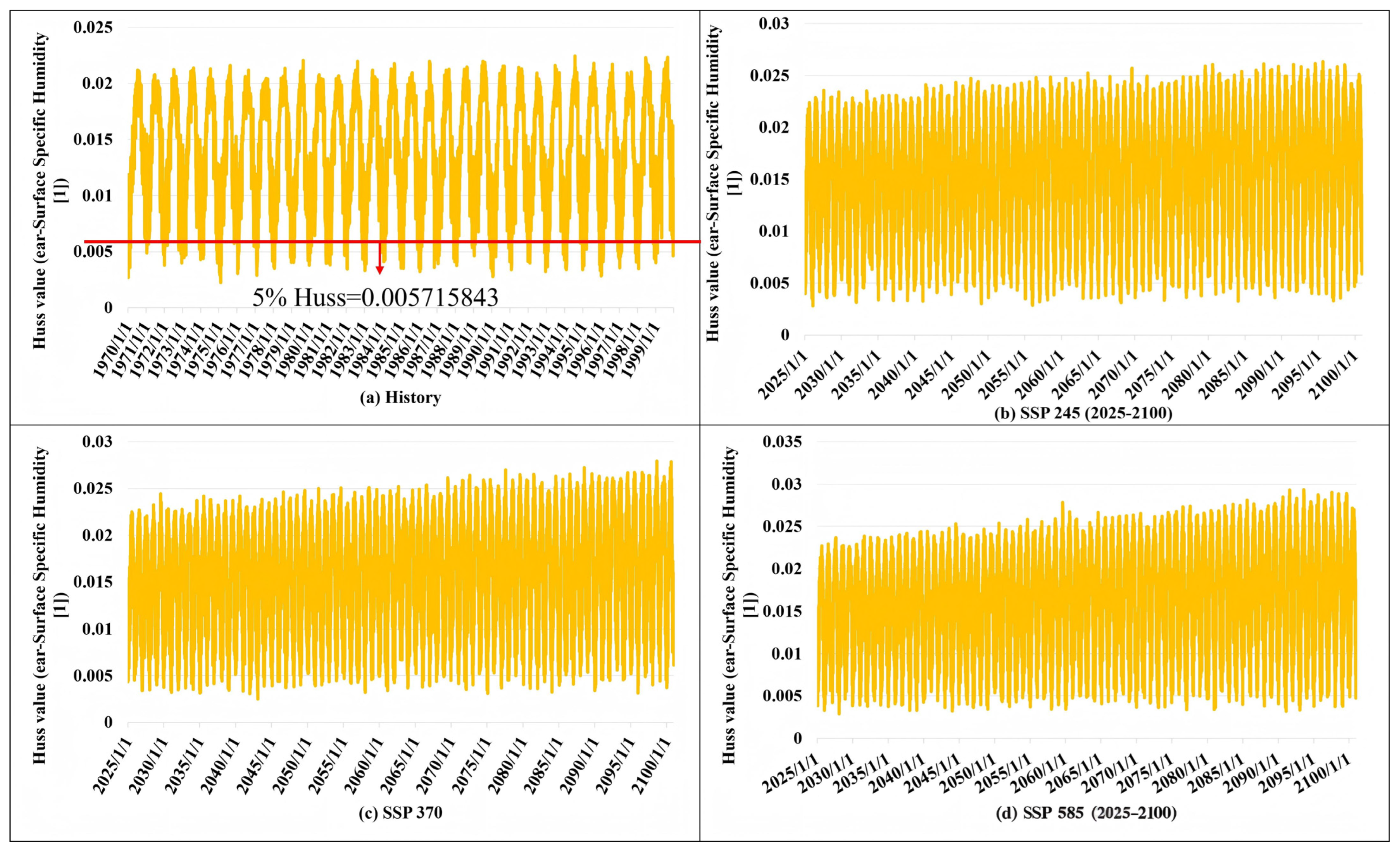
Our analysis focuses on Guangdong Province (20.2167°–25.5167° N, 109.75°–117.333° E), for which we extracted daily near-surface specific humidity (huss) data from 1970 to 1999 to establish the historical baseline, as well as for future scenarios under SSP245, SSP370, and SSP585. We define Extreme Drought Days (EDD) as days when huss falls below the 5th percentile of historical values, calculated to be 0.005715843 (Figure 1a).

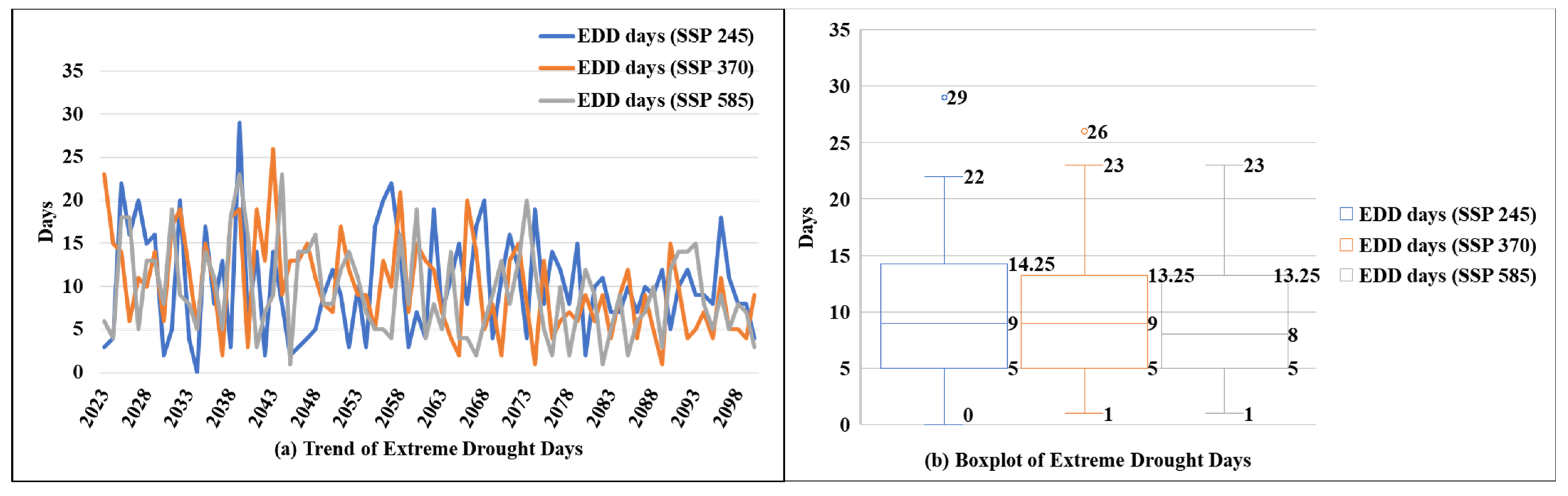
Under all three SSP scenarios, the frequency of EDD shows a declining trend between 2024 and 2100 (Figure 2a). The projected annual maximum number of EDD is 29 days for SSP245, 26 days for SSP370, and 23 days for SSP585. The 75th percentile values are 14.25, 13.25, and 13.25 days, respectively, while the median values are 9, 9, and 8 days. Notably, the 25th percentile remains constant at 5 days across all scenarios (Figure 2b). These results suggest a steady reduction in median drought intensity with increasing radiative forcing.

This observed trend likely reflects the intensification of the East Asian summer monsoon under warming conditions, which enhances the inflow of warm, humid air masses into southern China. As atmospheric moisture levels increase, the occurrence of extreme drought events declines. This outcome is consistent with theoretical expectations presented in Section 2.1 and may contribute to improved juvenile tilapia survival rates under future climate scenarios.

2.4. Parameters

To estimate the loss function for q, we apply a set of structural assumptions to the parameters of the production function (

Table 1. Parameters of Model.

Parameters	Value
α1	0.5
α2	0.25
α3	0.25
Pk	1
Pl	1
pqa	1
Ρ	−0.5

). Tilapia aquaculture in Guangdong Province is characterized by significant economies of scale, where economic returns are primarily driven by the intensive stocking of juvenile fish [39,40]. Accordingly, the production elasticity of juvenile fish input (α₁) is set to 0.5. In addition, we assume a fixed input ratio of 0.25 between labor and aquaculture area. The parameter (α₁) is set to 0.5 to reflect a balanced contribution of inputs under typical semi-intensive aquaculture conditions in China, and to provide a neutral benchmark in the absence of disaggregated empirical estimates, following standard calibration practices in economic modeling [18].

In order to isolate the biophysical and climate-related factors influencing production, we treat the price of juvenile tilapia (P_k), the wage rate for aquaculture labor (P_l), and the rental cost of aquaculture area (P_qa) as exogenous variables. All three prices are normalized to one. Following established practices in the literature [19,20], the elasticity of substitution among inputs (−ρ) is set to 0.5. Our decision to normalize all factor prices to unity was made to preserve dimensional consistency and isolate the effects of technical change, rather than to imply price homogeneity. In theoretical production analysis, normalization is a standard method used to abstract from nominal price variations when focusing on relative productivity or efficiency changes. Price normalization is applied as a scale transformation to simplify the model and ensure comparability. Since the model depends on relative prices rather than absolute values, this normalization does not affect the qualitative results [41,42]. The parameters reported in Table 1 are treated as benchmark calibrated values [41,43]. Sensitivity analysis is not conducted for all exogenous parameters but is focused on key structural parameters (r) and (η) that directly influence the drought–production transmission mechanism.

2.5. Production Data for Tilapia

To conduct the loss function of growth rate of tilapia aquaculture and probability of extreme drought risk factors, this study focuses on tilapia aquaculture in Guangdong Province, China, over the period 2003–2023. Data on total tilapia output (Q) and juvenile fish input (K) were obtained from the China Fishery Statistical Yearbook (2003–2024) (

Table 2. Tilapia Production Data in Guangdong Province, China (2003–2023).

Year	Q (100,000 Metric Tons)	K (One Billion Fish Fry)	L (Ten Thousand People)	QA (Ten Thousand Hectares)	A (--)	${\mathit{\tau }}_{\mathit{p}}$
2003	3.89145	5.6	5.1361	5.7489	0.9780	0.062424137
2004	4.3955	5.7	6.2657	6.1536	0.9850	0.098260101
2005	4.64711	5.8	6.2526	6.2160	0.9930	0.104502514
2006	5.25211	5.2	5.8009	6.7551	0.9960	0.077683371
2007	5.92712	5.5	9.2208	6.9961	1.0380	0.11375065
2008	5.17816	7.5	7.5107	6.2245	0.9970	0.12531056
2009	5.83996	9.0	8.3873	7.0858	1.0160	0.09987862
2010	6.24178	10.2	8.8186	7.2234	1.0210	0.076527484
2011	6.46080	10.3	8.6853	7.2217	1.1230	0.145425004
2012	6.64647	10.4	8.2771	7.2121	1.0510	0.043003295
2013	7.00219	11.4	7.8090	7.2390	1.0320	0.113519334
2014	7.14296	11.7	7.5016	7.1055	1.0110	0.085775273
2015	7.41188	11.7	7.5269	7.1100	1.0360	0.037454482
2016	7.75318	11.3	7.5522	7.0461	1.0990	0.0383794
2017	7.22625	10.5	7.4969	6.1002	1.1090	0.071672273
2018	7.51239	10.2	7.4338	6.1651	1.1440	0.075140281
2019	7.44022	10.2	7.0930	5.8259	1.1552	0.061961852
2020	7.40141	9.4	6.7944	5.5122	1.1664	0.06797295
2021	7.38715	7.9	6.9510	5.4434	1.1776	0.107508237
2022	7.56729	7.4	6.2681	5.4362	1.1888	0.091654586
2023	7.78471	7.5	7.1772	5.4194	1.2000	0.05697451

Note: ${\tau }_p$ represents the annual occurrence of extreme drought, derived from NOAA near-surface specific humidity (huss) data using a percentile-based threshold (5th percentile).

). The index of technological progress (A) was sourced from Yang [44] and Zhang [45], which adopt a nonlinear transformation of historical productivity trajectories to ensure smooth convergence. In our implementation, the transformation ensures that the asymptotic value (0.01477) represents a convergent annualized growth rate, consistent with the empirical slowdown observed in long-run TFP growth in technologically maturing sectors. The transform is logarithmic in form, applied to avoid abrupt slope changes. The convergence rate (0.01477) is calibrated to ensure continuity with the 2003–2030 historical average (approximately 1.45%). The value lies within the empirical range of long-term technological growth observed in industrial and agricultural productivity datasets [46]. A and η are parametric rather than statistical, and that ensemble dispersion should be interpreted as structural variation.

The number of specialized tilapia farmers (L) is not directly reported in the statistical yearbook and is therefore estimated using a proportional allocation approach based on output shares. This method is widely used in agricultural and fisheries studies when disaggregated input data are unavailable [47]. It was estimated as:

$$L=Number of specialized freshwater of fish farmers in Guangdong\times {\displaystyle \frac{Yield of Tilapia aquaculture in Guangdong}{Freshwater aquaculture yield in Guangdong}}$$

Similarly, tilapia aquaculture area (QA) is not explicitly provided and was calculated as:

$$QA=Yield of tilapia aquaculture\times {\displaystyle \frac{Freshwater aquaculture area in Guangdong}{Yield of freshwater in Guangdong}}$$

Given the scenario-based nature of the analysis, model validation is conducted using a multi-level approach, as conventional out-of-sample validation is not directly applicable in a mechanism-based simulation framework. Specifically, the model is evaluated through (i) comparison with historical observations, (ii) sensitivity analysis of key parameters, (iii) consistency with established climate–impact and bioeconomic modeling frameworks [48,49,50].

This study adopts a calibrated structural modeling framework, in which the primary objective is to capture the underlying production mechanisms and scenario-based dynamics rather than to optimize statistical fit. Accordingly, model performance is assessed based on the consistency between predicted and observed values, as well as the stability and distribution of residuals across alternative parameter settings.

In this context, traditional goodness-of-fit metrics such as R² or RMSE are not emphasized, as they are less informative for evaluating the structural validity and scenario-based performance of the model.

3. Results

3.1. Influence of Natural Growth Rate (r) and Extreme Drought Loss Parameter (η) on q

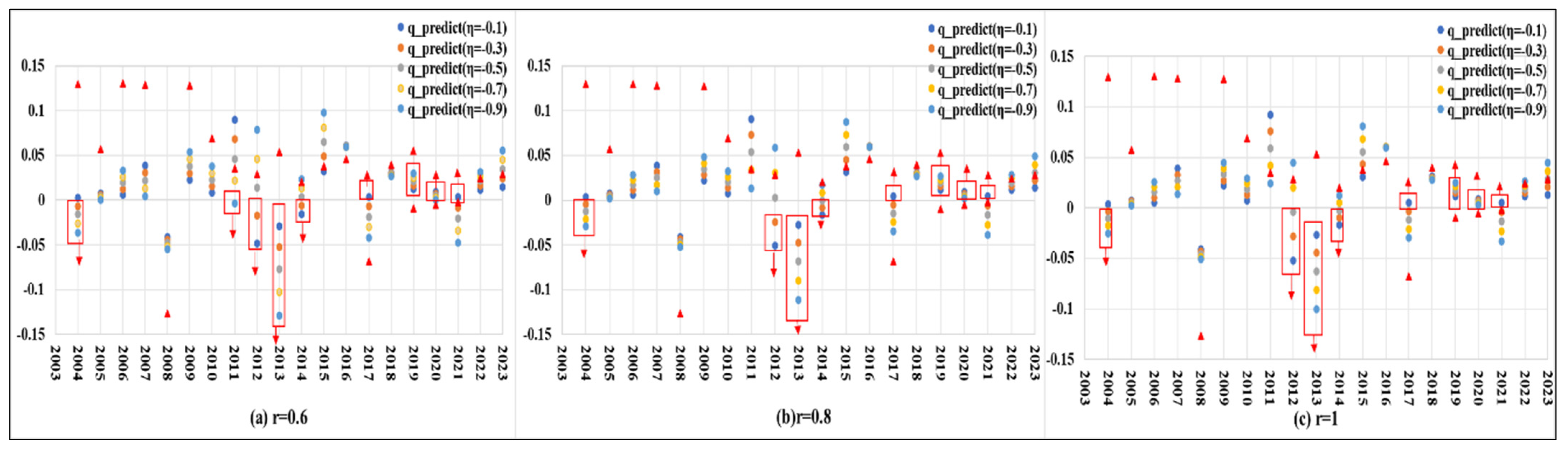
As shown in Figure 3a, when the natural growth rate is set to r = 0.6, noticeable divergence between predicted and observed values of q can be observed in several years. As r increases to 0.8 and 1 (Figure 3b,c), the magnitude of these deviations is reduced, indicating improved alignment between model simulations and observed trends. The largest discrepancies occur in 2004 and 2023, where the model predicts negative values while the observed values remain positive. This divergence reflects structural differences not fully captured by the model.

This divergence reflects factors outside the scope of the model rather than deficiencies in the model structure. The framework isolates the climate–production linkage through drought-induced changes in juvenile survival, while external influences such as technological progress, policy support, and adaptive management are not explicitly incorporated [39].

Accordingly, residuals are interpreted as structural residuals, capturing the net effect of these external drivers and clarifying the boundary between the internal model mechanism and real-world influences.

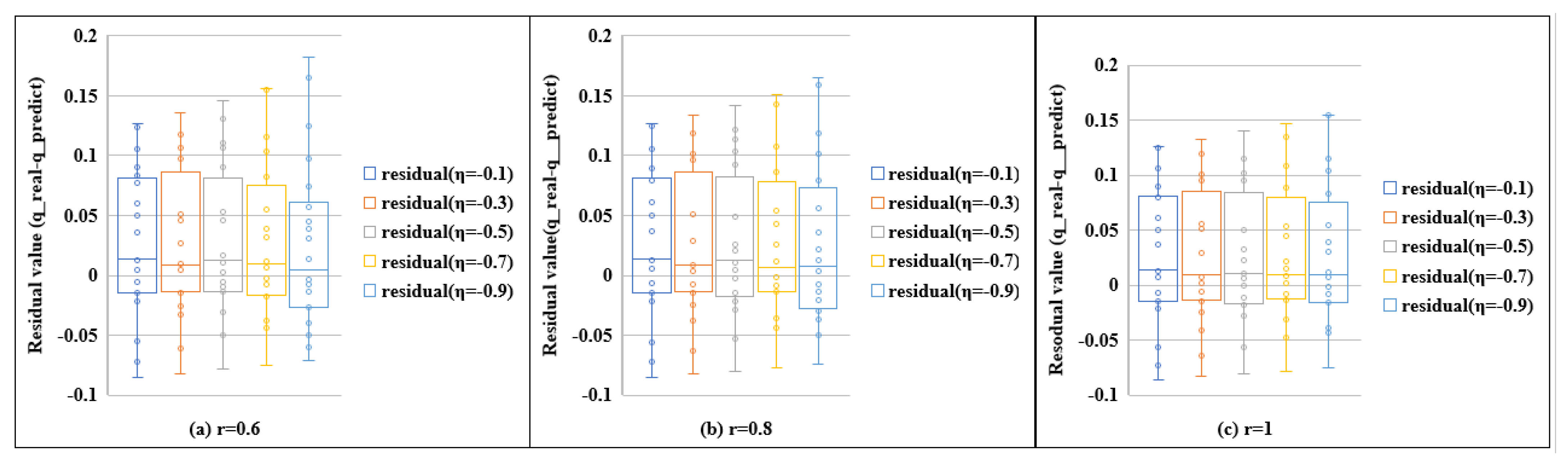
Figure 4a shows that under r = 0.6, increasing the absolute value of the extreme drought loss parameter η shifts the residual median closer to zero. For example, when η = −0.9, the median residual is approximately 0.005, indicating improved model consistency. Although the maximum residual increases, the absolute value of the minimum residual declines. Similar patterns are observed in Figure 4b,c. Across different values of r, both the maximum and minimum residuals decrease as r approaches 1, and the distribution becomes more concentrated, indicating improved model stability. Since η is treated as a scenario-based uncertainty parameter rather than an estimable coefficient [16,17]. These results reflect structural model responses rather than statistical estimation outcomes.

The parameter r is treated as a structural parameter rather than a directly measurable biological coefficient. Simulations under r = 0.6, 0.8, and 1 show improved model performance as r increases, with reduced divergence and more concentrated residuals. Accordingly, r = 1 is adopted as the benchmark specification, as it provides the best empirical fit while preserving the robustness of qualitative results.

Consistent with Figure 3 and Figure 4, this choice provides a reasonable representation of the natural growth rate of tilapia. Given the asymmetric effects of η on the residual distribution of q, multiple values of η are incorporated to capture the range of potential variability in climate-induced production loss.

3.2. Loss Function of q

Building on the formulation presented in Section 2.1, and using the variables and parameters specified in Table 1 and Table 2, the loss function for q is defined under the assumption that the natural growth rate r equals 1. Five discrete levels of the extreme drought loss parameter η are considered in the analysis, including η = −0.1, −0.3, −0.5 −0.7, and −0.9. The corresponding functional forms of the loss function are presented in Figure 5. Specifically, the loss functions are as follows:

$$\begin{array}{l}q=a-0.113257d\tau when \eta =-0.1\\ q=a-0.342659d\tau when \eta =-0.3\\ q=a-0.576062d\tau when \eta =-0.5\\ q=a-0.813647d\tau when \eta =-0.7\\ q=a-1.055609d\tau when \eta =-0.9\end{array}$$

(24)

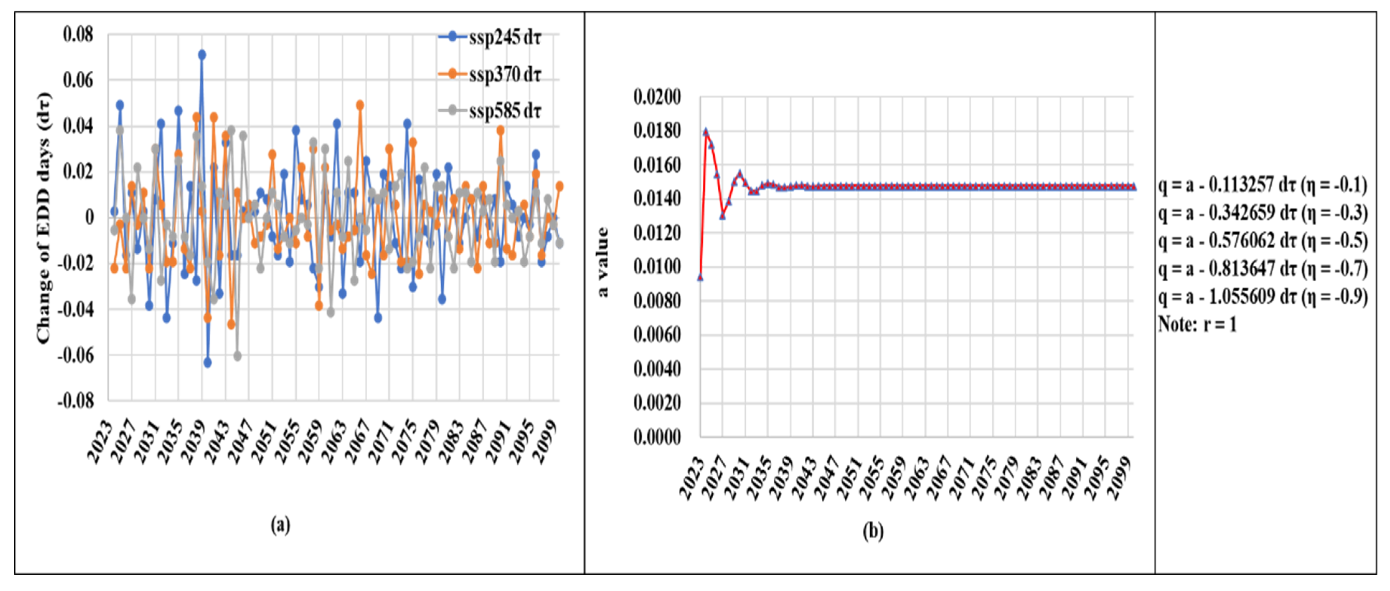
To estimate future values of the tilapia yield growth rate q and the corresponding total output Q under the SSP245, SSP370, and SSP585 scenarios, this study follows by calculating the change in the probability of the climate drought risk factor (dτ) and the rate of technological progress (a) over the period from 2024 to 2100. The variable dτ is derived from observed shifts in the probability of extreme drought, as illustrated in Figure 2. The technological progress rate a is estimated based on an average-growth-rate-based forecasting model (Figure 5).

Figure 5a shows that the amplitude of fluctuations in dτ gradually decreases across all scenarios throughout the study period. This pattern suggests a long-term weakening in the frequency and variability of extreme drought events. In contrast, Figure 5b demonstrates that the growth rate of technological progress a experiences considerable variation between 2024 and 2030 but becomes increasingly stable after that period. From 2031 to 2100, a converges toward an average value of approximately 0.01477, indicating a consistent and sustained pace of technological advancement during the latter half of the century.

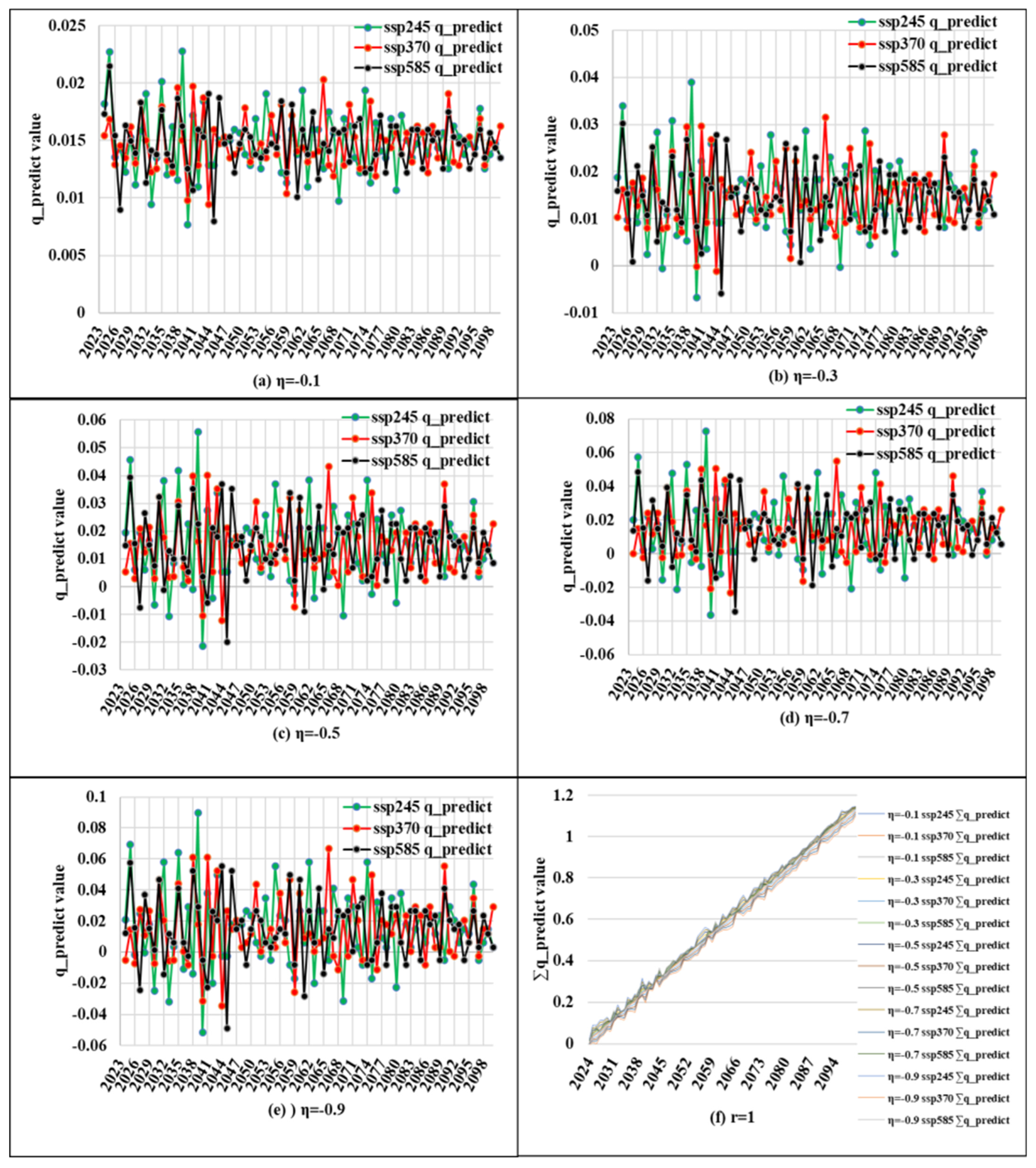
As illustrated in Figure 6a, under a relatively mild drought impact parameter (η = −0.1), the tilapia yield growth rate (q) remains positive throughout the entire simulation period. Cumulative growth in q by 2100 is substantially higher under SSP245 (1.4422) compared to SSP370 (1.1376) and SSP585 (1.1410), as shown in Figure 6f. Across all scenarios, the cumulative growth in technological progress (a) is held constant at 1.1419. The additional gain under SSP245, amounting to approximately 0.0003, is attributable to a more pronounced decline in extreme drought risk, likely reducing juvenile mortality and enhancing productivity.

These results indicate that under current socioeconomic and emission trajectories, warming-induced reductions in drought frequency are likely to confer modest benefits to aquaculture in Guangdong. In contrast, under SSP370 and SSP585, the contributions of drought risk reduction to cumulative q become slightly negative (−0.0043 and −0.0009, respectively), reflecting slower improvements in drought conditions and diminished marginal gains. However, the magnitude of these effects is negligible and unlikely to pose a significant constraint on production.

Figure 6f further demonstrates that under higher values of drought sensitivity (η = −0.3, −0.5, −0.7, −0.9), the advantage of SSP245 becomes more pronounced, with consistent positive contributions to cumulative q (ranging from 0.0009 to 0.0029). In contrast, SSP370 and SSP585 exhibit increasingly negative effects, with contributions ranging from −0.0131 to −0.0405 and −0.0028 to −0.0087, respectively.

Figure 6b–e highlight the temporal dimension of these dynamics. As drought sensitivity intensifies, the probability of annual yield decline increases. Under SSP245, no negative values of q are observed when η = −0.1; however, the number of years with yield decline rises to 3, 9, 17, and 22 for η = −0.3, −0.5, −0.7, and −0.9, respectively. This suggests that increased vulnerability to drought diminishes the productivity gains associated with a reduced drought frequency.

Moreover, for any fixed value of η, increasing radiative forcing across SSPs amplifies inter annual variability in extreme drought, introducing greater uncertainty into aquaculture outcomes. While lower emission scenarios benefit from more consistent reductions in drought risk, SSP370 and SSP585 are associated with higher volatility. For instance, when η = −0.3, the number of years with negative q is 3 under SSP245, 2 under SSP370, and 1 under SSP585; when η = −0.9, these values increase to 22, 17, and 17, respectively.

Taken together, these results suggest that the projected decline in drought frequency under SSP245 could facilitate the sustainable expansion of tilapia aquaculture in Guangdong by the end of the century. While SSP370 and SSP585 are associated with slightly negative contributions from drought risk reduction, the effects are limited in magnitude. Overall, climate warming is unlikely to impose major biophysical constraints on tilapia production through drought-related mechanisms alone, although other environmental stressors may still play an important role.

3.3. Projected Yield (Q) of Tilapia

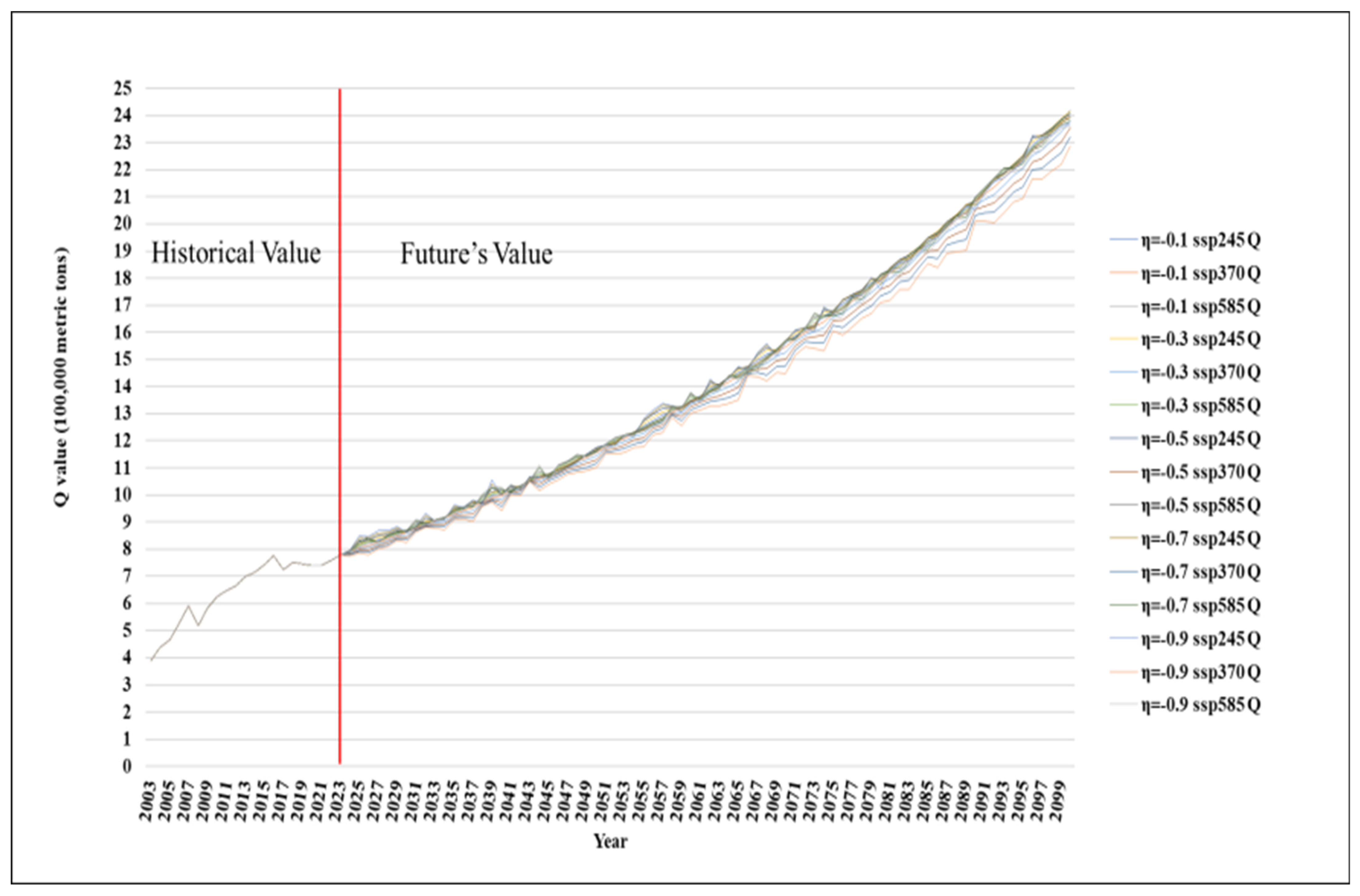
The SSP370 and SSP585 scenarios have the potential for a minimal negative impact on tilapia aquaculture in Guangdong, as discussed in Section 3.2. Under SSP245, a reduction in drought frequency may even result in enhanced production outcomes. To provide a more intuitive representation of these effects, annual tilapia yield is simulated (Q) from 2024 to 2100 based on the previously estimated yield growth rate (q), as shown in Figure 7.

Figure 7 demonstrates that the projected values of Q closely align with historical production data, exhibiting no abrupt deviations. This correspondence supports the internal consistency and empirical robustness of the q loss function. From 2024 to 2075, increases in annual yield remain modest across all scenarios. However, from 2076 onward, the growth rate accelerates markedly. The sustained increase in tilapia production is due to the decrease in extreme drought frequency after 2075, as well as steady technological advancement.

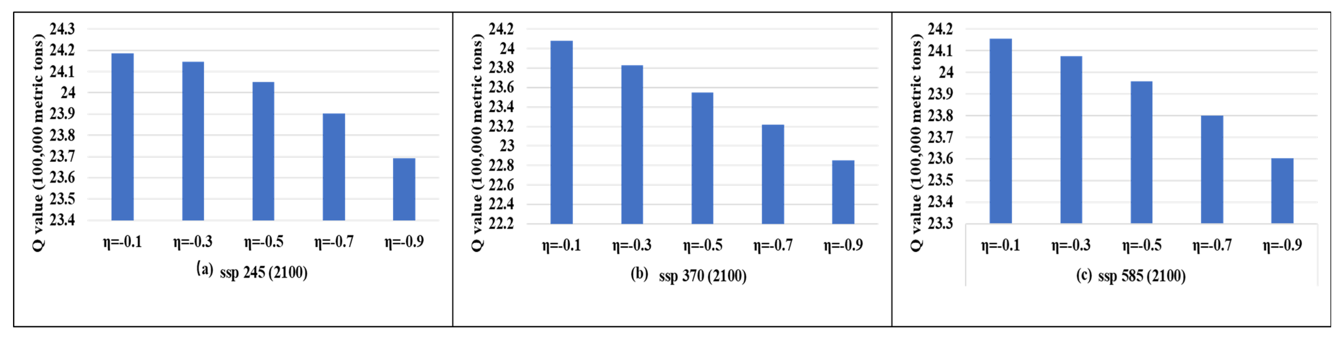
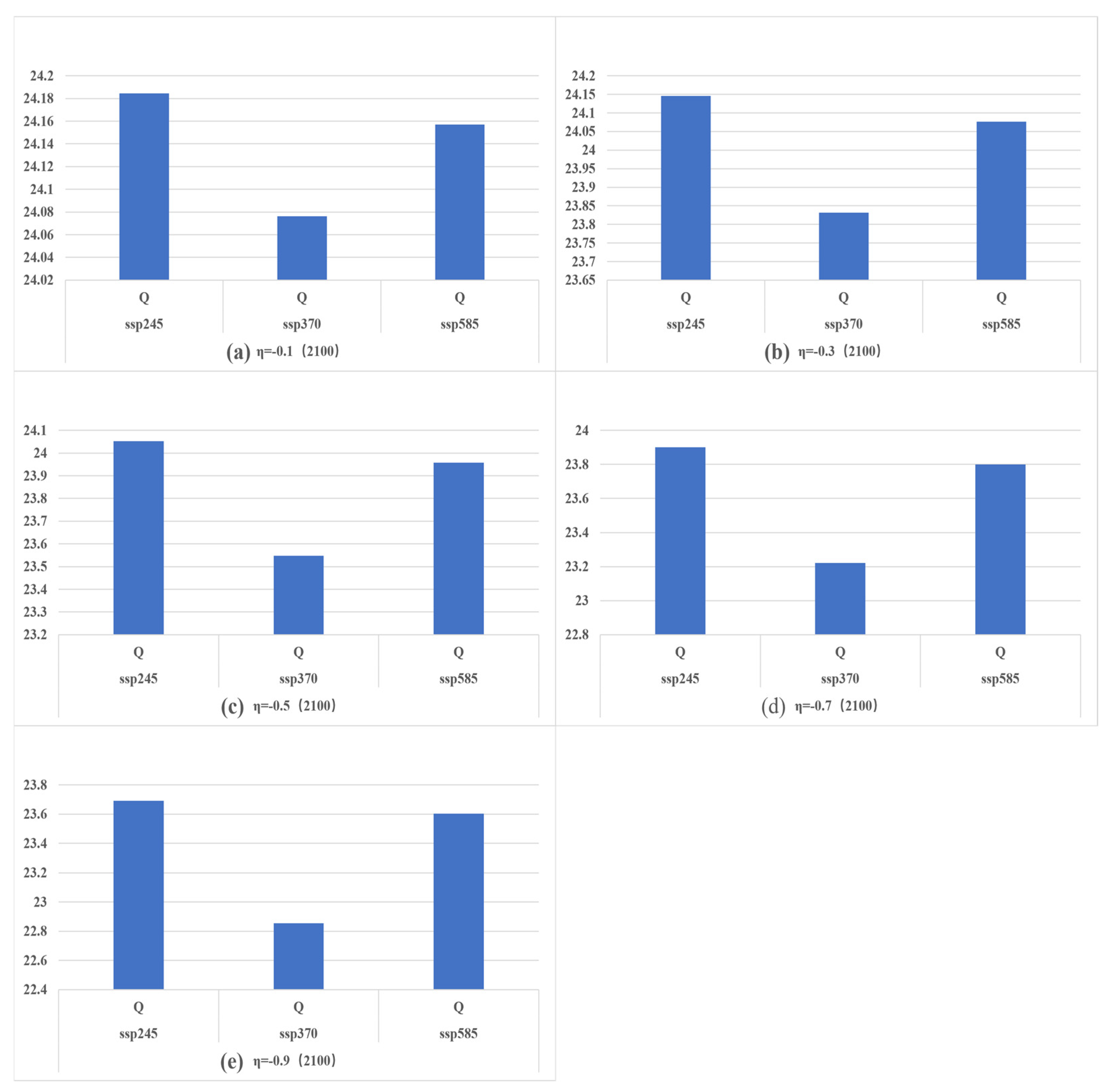
Figure 8 illustrates how yield projections respond to variation in the extreme drought loss parameter (η) within each climate scenario. Under SSP245, when η = −0.1, yield is projected to reach 2.418 million tons. Increasing drought sensitivity to η = −0.9 results in a yield reduction of 49,400 tons. Under SSP370, yield declines from 2.407 to 2.395 million tons, a difference of 12,200 tons. In SSP585, the corresponding decline is 5600 tons, from 2.416 to 2.410 million tons. These results confirm that higher drought sensitivity consistently reduces yield across all climate pathways, with the most pronounced effects observed under SSP245.

Figure 9 explores yield patterns under constant drought sensitivity and varying levels of radiative forcing. Scenarios show a distinct U-shaped trajectory. For instance, when η = −0.1, yield decreases from 2.418 million tons in SSP245 to 2.408 million tons in SSP370, before rising to 2.416 million tons in SSP585. This represents a recovery of 0.8 million tons between SSP370 and SSP585. A similar pattern is observed under higher drought sensitivity. When η = −0.9, yield falls from 2.369 million tons in SSP245 to 2.286 million tons in SSP370, then rebounds to 2.360 million tons in SSP585, representing a net increase of 7.4 million tons relative to SSP370.

The observed U-shaped response is primarily driven by the marginal effects of changes in the probability of extreme drought risk (dτ) across different climate regimes. While SSP245 is associated with a gradual decline in drought frequency, SSP370 exhibits both increased atmospheric humidity and lower variability in drought occurrence. This combination reduces the marginal benefits of further drought risk reduction. In contrast, SSP585 is characterized by heightened interannual variability and greater extremes in drought conditions. This enhances the marginal responsiveness of production to changes in dτ, contributing to the observed rebound in projected yield. The observed “U-shaped” yield response (with a relative advantage under SSP245) arises from the interaction between moderate warming-induced productivity gains and high-end stress-related losses, rather than from statistical differences across scenarios. Specifically, the pattern reflects a mechanism-driven nonlinear response, in which moderate climate change improves production conditions, while higher levels of forcing introduce stress effects that reduce productivity. This interpretation aligns with prior studies showing that intermediate climate forcing scenarios may produce relatively favorable economic or biophysical outcomes due to nonlinear threshold responses and diminishing marginal impacts of environmental stress [51,52,53].

The results presented here isolate and quantify the marginal biophysical effect of changes in drought frequency on yield potential. They are not intended as a full-system forecast encompassing heat-induced mortality, pathogen dynamics, or eutrophication feedbacks. Accordingly, these findings should be interpreted as illustrative of a single mechanistic pathway within the broader coupled climate–water quality–disease system. Within this framework, technological progress (A) accounts for approximately 80% of the total variation in projected yield, representing the dominant structural driver. In contrast, the climatic component contributes second-order fluctuations, primarily modulated by drought frequency and temperature anomalies. The consistency of relative contributions across SSPs further suggests a degree of structural robustness, even in the absence of formal statistical confidence intervals.

4. Discussion

This inter-model uncertainty is a key challenge in climate impact assessment. CMIP-based studies consistently report substantial variability across models, but do not provide a unified numerical range. Instead, differences are typically described in relative terms (high, medium, and low response models), reflecting variations in model structure and physical processes [54,55,56].

In this study, uncertainty is represented using a scenario-based approach. Previous work suggests that inter-model differences in CMIP ensembles are typically on the order of tens of percent, with uncertainties in projected changes often reaching 10–30% or higher depending on the variable and region [57,58,59]. Based on this, a 10–30% range is adopted to represent moderate uncertainty. This range is not intended to match specific model outputs, but to capture the central variability implied by multi-model comparisons. Three scenarios (high, medium, and low) are constructed using representative model types. High-response models show stronger moisture increases, while low-response models are more conservative. TaiESM1 is used as the baseline representing intermediate behavior.

Differences in near-surface humidity (

Table 3. Assumed scenarios of near-surface specific humidity (huss) under three climate response regimes.

Uncertainty Level	Model	Relative Change (%)	Absolute Huss Difference (Δhuss, g kg−1)	Interpretation
HIGH	IPSL-CM6A-LR	+20% to +30%	+3 to +6	Strong convection and evapotranspiration → wetter bias
	UKESM1-0-LL	+20% to +30%	+3 to +6	Strong aerosol–cloud feedback enhances moisture variability
	CanESM5	+15% to +25%	+2 to +5	High climate sensitivity → stronger hydrological amplification
	CESM2	+15% to +20%	+2 to +4	Strong warming → enhanced moisture increase
MEDIUM	TaiESM1	0%	0	Representative ensemble mean behavior
	GFDL-ESM4	−5% to +10%	−1 to +2	Balanced hydrological processes
	MIROC6	−5% to +10%	−1 to +2	Close to ensemble mean
	MRI-ESM2-0	−5% to −15%	−1 to −3	Moderately conservative response
LOW	MPI-ESM1-2-LR	−15% to −25%	−2 to −5	Conservative water cycle
	NorESM2-MM	−10% to −20%	−2 to −4	Lower hydrological sensitivity

Note: Δhuss = U_rel × huss_clim. U_rel is Relative Change (%). huss_clim is 10–30%.

) lead to corresponding changes in drought frequency (

Table 4. Changes in Extreme Drought Days (Δτ) under three climate response regimes.

Uncertainty Level	Model	Relative Change (%)	Δτ (Days/Year)
HIGH	IPSL-CM6A-LR	−20% to −40%	−6 to −15
	UKESM1-0-LL	−20% to −40%	−6 to −15
	CanESM5	−15% to −30%	−4 to −12
	CESM2	−15% to −25%	−4 to −10
MEDIUM	TaiESM1	−10% to −20%	−2 to −8
	GFDL-ESM4	−5% to −15%	−1 to −6
	MIROC6	−5% to −15%	−1 to −6
	MRI-ESM2-0	−5% to −20%	−1 to −8
LOW	MPI-ESM1-2-LR	−5% to −10%	−1 to −4
	NorESM2-MM	−5% to −10%	−1 to −4

Note: Δτ = U_rel × τ_clim. τ_clim is days of TaiESM1.

). High-response scenarios show larger reductions (−6 to −15 days), while low-response scenarios show smaller changes (−1 to −4 days). These differences further propagate to production (

Table 5. Propagation from Drought (Δτ) to Yield (q) and Production (Q) under three climate response regimes.

Model Level	Δτ (Days/Year)	Impact on q (%)	Impact on Q (%)	Mechanism
HIGH	−4 to −15	+4% to +15%	+4% to +15%	Strong drought reduction improves survival
MEDIUM	−1 to −8	+1% to +8%	+1% to +8%	Balanced moisture change
LOW	−1 to −4	0% to +4%	0% to +4%	Minimal hydrological change

Note: q = f(τ); Q = A·q.

), where higher drought reduction leads to larger increases in yield (q) and total production (Q).

Table 5 indicates that reductions in extreme drought days (Δτ) lead to consistent increases in yield (q) and production (Q), with the magnitude varying across scenarios. Under the high-response regime, larger drought reductions (−4 to −15 days) result in substantial gains (4–15%), reflecting improved survival and more stable growing conditions. In the medium scenario, moderate reductions (−1 to −8 days) produce intermediate gains (1–8%), representing the central system response. In contrast, the low-response scenario shows only limited improvements (0–4%) due to minimal hydrological change. Overall, the relationship is positive but nonlinear, with diminishing marginal gains as drought conditions continue to weaken.

5. Conclusions

This study develops a loss function that links extreme drought risk to juvenile tilapia survival, enabling quantification of the impacts of drought variability on aquaculture yield growth. By integrating this function with climate projections from the TaiESM1 model under the CMIP6 framework, we simulate the potential evolution of tilapia production in Guangdong Province from 2024 to 2100. The main findings can be summarized as follows:

(1). Decline in extreme drought frequency: Across all SSP scenarios (SSP245, SSP370, and SSP585), the frequency of extreme drought events in Guangdong is projected to decline. This simulated trend is consistent with the expected increase in atmospheric moisture under warming conditions and is supported by CMIP6-based studies. However, increased variability and the risk of drought–flood alternation may still pose challenges for aquaculture management.

(2). Differentiated effects of emission scenarios: Under SSP245, the simulated decline in drought risk tends to support yield growth. Under SSP370 and SSP585, the marginal benefits are smaller due to stronger radiative forcing and increased variability. However, the magnitude of these differences remains relatively limited within the modeling framework.

(3). Sensitivity to loss parameters: The simulated effects of drought reduction depend on the assumed loss parameter (η). Under lower sensitivity, reductions in drought risk are associated with more favorable production outcomes, while higher sensitivity reduces these gains. This highlights the importance of management capacity and adaptation in shaping aquaculture resilience.

(4). Nonlinear response across SSPs: Tilapia yield exhibits a nonlinear (U-shaped) response across emission scenarios in the simulations, reflecting differences in the variability and marginal effects of drought risk. This suggests that climate–production relationships are scenario-dependent and subject to diminishing marginal responses.

Based on the findings of this study, several adaptive management implications can be drawn for tilapia aquaculture in Guangdong Province, China. First, strengthening water resource governance is essential for mitigating drought-induced production risks, particularly through improving allocation efficiency and enhancing monitoring of hydrological conditions relevant to aquaculture systems. Second, reinforcing technology-based adaptation is critical for sustaining production under environmental stress, with emphasis on improving production efficiency and stabilizing key biological processes. Third, developing targeted risk-buffering mechanisms is necessary to reduce climate-induced variability, thereby enhancing the stability and resilience of aquaculture production systems.

However, this framework does not encompass the full spectrum of biophysical feedbacks involving heatwaves, stratification, eutrophication, or disease dynamics. Instead, it isolates the effect of atmospheric dryness (via huss-defined drought) within a simplified modeling context. Future research could further extend this framework by incorporating additional dimensions of climate and environmental variability and by enhancing the representation of system complexity.

References

1. Asritha, A.; Nischal, L.; Rao, A.C.S.; Reddy, B.S.K.; Kumar, E.V.; Lavanya, C.; Sirisha, H.; Ratnasree, A.; Sadu, H.; Ganesh, G. Change in Climate and Its Impact on Aquaculture Sector. Uttar Pradesh J. Zool. 2024, 45, 230–242. [Google Scholar] [CrossRef]
2. Formento, C.Z.D.; Dulaca, M.N.M.B.; Rojas-Salinas, A.; Cortes, J.R. Climate-Related Risk Management Practices in Pond-Based Tilapia Culture: A Case Study of the Small-Scale Fish Farmers of Agusan Del Sur, Philippines. BIO Web Conf. 2023, 74, 01014. [Google Scholar] [CrossRef]
3. Lebel, P.; Whangchai, N.; Chitmanat, C.; Lebel, L. Risk of Impacts from Extreme Weather and Climate in River-Based Tilapia Cage Culture in Northern Thailand. Int. J. Glob. Warm. 2015, 8, 534. [Google Scholar] [CrossRef]
4. Pimolrat, P.; Whangchai, N.; Chitmanat, C.; Promya, J.; Lebel, L. Survey of Climate-Related Risks to Tilapia Pond Farms in Northern Thailand. Int. J. Geosci. 2013, 4, 54–59. [Google Scholar] [CrossRef]
5. Ribeiro, O.; Pinto, M.Q.; Tavares, D.; Ferreira-Cardoso, J.V.; Correia, A.T.; Carrola, J.S. Copper and Temperature Interaction Induced Gill and Liver Lesions and Behaviour Alterations in Mozambique Tilapia (Oreochromis mossambicus). Water 2024, 16, 2499. [Google Scholar] [CrossRef]
6. Liao, P.-C.; Tsai, Y.-L.; Chen, Y.-C.; Wang, P.-C.; Liu, S.-C.; Chen, S.-C. Analysis of Streptococcal Infection and Correlation with Climatic Factors in Cultured Tilapia Oreochromis spp. in Taiwan. Appl. Sci. 2020, 10, 4018. [Google Scholar] [CrossRef]
7. Wang, K.; Niu, J.; Li, T.; Zhou, Y. Facing Water Stress in a Changing Climate: A Case Study of Drought Risk Analysis Under Future Climate Projections in the Xi River Basin, China. Front. Earth Sci. 2020, 8, 86. [Google Scholar] [CrossRef]
8. Mehta, T.K.; Man, A.; Ciezarek, A.; Ranson, K.; Penman, D.; Di-Palma, F.; Haerty, W. Chromatin Accessibility in Gill Tissue Identifies Candidate Genes and Loci Associated with Aquaculture Relevant Traits in Tilapia. Genomics 2023, 115, 110633. [Google Scholar] [CrossRef]
9. Tran, N.; Cao, Q.L.; Shikuku, K.M.; Phan, T.P.; Banks, L.K. Profitability and Perceived Resilience Benefits of Integrated Shrimp-Tilapia-Seaweed Aquaculture in North Central Coast, Vietnam. Mar. Policy 2020, 120, 104153. [Google Scholar] [CrossRef]
10. Chua, V.L.; Carillo, F.R., Jr. Development of Magallanes Tilapia (Tilapia mossambica) Tocino Project: Its Processing, Verification, Commercialization and Utilization. IAMURE Int. J. Math. Eng. Technol. 2012, 4, 1–7. [Google Scholar] [CrossRef]
11. Uppanunchai, A.; Chitmanat, C.; Lebel, L. Mainstreaming Climate Change Adaptation into Inland Aquaculture Policies in Thailand. Clim. Policy 2018, 18, 86–98. [Google Scholar] [CrossRef]
12. Challinor, A.J.; Watson, J.; Lobell, D.B.; Howden, S.M.; Smith, D.R.; Chhetri, N. A Meta-Analysis of Crop Yield under Climate Change and Adaptation. Nat. Clim. Change 2014, 4, 287–291. [Google Scholar] [CrossRef]
13. Knox, J.; Hess, T.; Daccache, A.; Wheeler, T. Climate Change Impacts on Crop Productivity in Africa and South Asia. Environ. Res. Lett. 2012, 7, 034032. [Google Scholar] [CrossRef]
14. Estes, L.D.; Beukes, H.; Bradley, B.A.; Debats, S.R.; Oppenheimer, M.; Ruane, A.C.; Schulze, R.; Tadross, M. Projected Climate Impacts to South African Maize and Wheat Production in 2055: A Comparison of Empirical and Mechanistic Modeling Approaches. Glob. Change Biol. 2013, 19, 3762–3774. [Google Scholar] [CrossRef]
15. Müller, C.; Cramer, W.; Hare, W.L.; Lotze-Campen, H. Climate Change Risks for African Agriculture. Proc. Natl. Acad. Sci. USA 2011, 108, 4313–4315. [Google Scholar] [CrossRef]
16. Nordhaus, W. Estimates of the Social Cost of Carbon: Concepts and Results from the DICE-2013R Model and Alternative Approaches. J. Assoc. Environ. Resour. Econ. 2014, 1, 273–312. [Google Scholar] [CrossRef]
17. Burke, M.; Hsiang, S.M.; Miguel, E. Global Non-Linear Effect of Temperature on Economic Production. Nature 2015, 527, 235–239. [Google Scholar] [CrossRef] [PubMed]
18. Arrow, K.J.; Chenery, H.B.; Minhas, B.S.; Solow, R.M. Capital-Labor Substitution and Economic Efficiency. Rev. Econ. Stat. 1961, 43, 225. [Google Scholar] [CrossRef]
19. Wei, T. Estimates of Substitution Elasticities and Factor-Augmented Technical Changes. SSRN J. 2014. [Google Scholar] [CrossRef]
20. Brubaker, E.R. Synthetic Factor Shares, The Elasticity of Substitution, and the Residual in Soviet Growth. Rev. Econ. Stat. 1970, 52, 100. [Google Scholar] [CrossRef]
21. Campbell, H.F. Estimating the Elasticity of Substitution between Restricted and Unrestricted Inputs in a Regulated Fishery: A Probit Approach. J. Environ. Econ. Manag. 1991, 20, 262–274. [Google Scholar] [CrossRef]
22. Ibáñez, A.L.; Torres-Vázquez, T.; Álvarez-Hernández, S.H. The Effect of High Temperature on the Growth Performance of Hybrid Tilapia Oreochromis niloticus X Oreochromis Aureus Juveniles Reared in a Recycling System. Annu. Res. Rev. Biol. 2019, 32, 1–8. [Google Scholar] [CrossRef]
23. Alemayehu, T.A.; Getahun, A. Effect of Feeding Frequency on Growth Performance and Survival of Nile Tilapia (Oreochromis niloticus L. 1758) in a Cage Culture System in Lake Hora-Arsedi, Ethiopia. J. Aquac. Res. Dev. 2017, 8, 1000479. [Google Scholar] [CrossRef]
24. Rahman, M.L.; Shahjahan, M.; Ahmed, N. Tilapia Farming in Bangladesh: Adaptation to Climate Change. Sustainability 2021, 13, 7657. [Google Scholar] [CrossRef]
25. Martinho, F.; Leitão, R.; Viegas, I.; Dolbeth, M.; Neto, J.M.; Cabral, H.N.; Pardal, M.A. The Influence of an Extreme Drought Event in the Fish Community of a Southern Europe Temperate Estuary. Estuar. Coast. Shelf Sci. 2007, 75, 537–546. [Google Scholar] [CrossRef]
26. White, R.S.A.; McHugh, P.A.; McIntosh, A.R. Drought Survival Is a Threshold Function of Habitat Size and Population Density in a Fish Metapopulation. Glob. Change Biol. 2016, 22, 3341–3348. [Google Scholar] [CrossRef]
27. Nordhaus, W.D. A Question of Balance: Weighing the Options on Global Warming Policies; Yale University Press: New Haven, CT, USA, 2008. [Google Scholar]
28. Lobell, D.B.; Schlenker, W.; Costa-Roberts, J. Climate Trends and Global Crop Production Since 1980. Science 2011, 333, 616–620. [Google Scholar] [CrossRef]
29. Guo, K.; Ji, Q.; Zhang, D. A Dataset to Measure Global Climate Physical Risk. Data Brief 2024, 54, 110502. [Google Scholar] [CrossRef]
30. Vicente-Serrano, S.M.; Beguería, S.; López-Moreno, J.I. A Multiscalar Drought Index Sensitive to Global Warming: The Standardized Precipitation Evapotranspiration Index. J. Clim. 2010, 23, 1696–1718. [Google Scholar] [CrossRef]
31. Dai, Y.; Zhou, Z.; Zhao, H.; Yu, Y.; Xu, X. Analysis of Chinese Tilapia Supply and Demand without and with the COVID-19 Epidemic Impact. Isr. J. Aquac. Bamidgeh 2022, 74, 1–10. [Google Scholar] [CrossRef]
32. Sheffield, J.; Wood, E.F.; Roderick, M.L. Little Change in Global Drought over the Past 60 Years. Nature 2012, 491, 435–438. [Google Scholar] [CrossRef]
33. Boyd, C.E. Water Quality: An Introduction; Springer International Publishing: Cham, Switzerland, 2015. [Google Scholar]
34. McKee, T.B.; Doesken, N.J.; Kleist, J. The Relationship of Drought Frequency and Duration to Time Scales. In Proceedings of the 8th Conference on Applied Climatology, Anaheim, CA, USA, 17–22 January 1993; pp. 179–184. [Google Scholar]
35. World Meteorological Organization (WMO). Handbook of Drought Indicators and Indices; WMO-No. 1173; WMO: Geneva, Switzerland, 2016. [Google Scholar]
36. Zhang, X.; Alexander, L.; Hegerl, G.C.; Jones, P.; Tank, A.K.; Peterson, T.C.; Trewin, B.; Zwiers, F.W. Indices for Monitoring Changes in Extremes Based on Daily Temperature and Precipitation Data. WIREs Clim. Change 2011, 2, 851–870. [Google Scholar] [CrossRef]
37. Dunn, R.J.H.; Morice, C.P. On the Effect of Reference Periods on Trends in Percentile-Based Extreme Temperature Indices. Environ. Res. Lett. 2022, 17, 034026. [Google Scholar] [CrossRef]
38. Di Bernardino, A.; Casadio, S.; Iannarelli, A.M.; Siani, A.M. Temperature Trends and Influence of the Base Period Selection on Climate Indices in the Mediterranean Region Over the Period 1961–2020. Int. J. Clim. 2024, 44, 5969–5985. [Google Scholar] [CrossRef]
39. Gu, D.E.; Yu, F.D.; Yang, Y.X.; Xu, M.; Wei, H.; Luo, D.; Mu, X.D.; Hu, Y.C. Tilapia Fisheries in Guangdong Province, China: Socio-economic Benefits, and Threats on Native Ecosystems and Economics. Fish. Manag. Ecol. 2019, 26, 97–107. [Google Scholar] [CrossRef]
40. Burad-Méndez, A.; Domínguez-May, R.; Olvera-Novoa, M.A.; Robledo, D.; Salas, S. Economic Analysis of Nile Tilapia (Oreochromis niloticus) Production Based on Farm Size and Number of Rearing Tanks. Lat. Am. J. Aquat. Res. 2023, 51, 747–759. [Google Scholar] [CrossRef]
41. Dawkins, C.; Srinivasan, T.N.; Whalley, J. Calibration. In Handbook of Econometrics; Elsevier: Amsterdam, The Netherlands, 2001; Volume 5, pp. 3653–3703. [Google Scholar]
42. Shoven, J.B.; Whalley, J. Applying General Equilibrium; Cambridge University Press: Cambridge, UK, 1992. [Google Scholar]
43. Hansen, L.P.; Heckman, J.J. The Empirical Foundations of Calibration. J. Econ. Perspect. 1996, 10, 87–104. [Google Scholar] [CrossRef]
44. Yang, Z.J. Measurement of TFP Assessing Contribution of Technological Progress to Chinese Fisheries Development. 2011 Annual Academic Conference of the Chinese Fisheries Society. 2011. Available online: https://cpfd.cnki.com.cn/Article/CPFDTOTAL-OGSB201111001594.htm (accessed on 15 November 2011).
45. Zhang, T.T. Research on the Changes in Total Factor Productivity and Regional Convergence of China’s Fishery Sector. Master’s Thesis, Zhejiang Ocean University, Zhoushan, China, 2021. Available online: https://d.wanfangdata.com.cn/thesis/Y3886472 (accessed on 23 February 2022).
46. Uribe, M.; Yue, V.Z. Country Spreads and Emerging Countries: Who Drives Whom? J. Int. Econ. 2006, 69, 6–36. [Google Scholar] [CrossRef]
47. Fuglie, K. Accounting for Growth in Global Agriculture. Bio-Based Appl. Econ. 2015, 4, 201–234. [Google Scholar] [CrossRef]
48. IPCC. Climate Change 2014: Impacts, Adaptation, and Vulnerability; Cambridge University Press: Cambridge, UK, 2014. [Google Scholar]
49. Pindyck, R.S. The Use and Misuse of Models for Climate Policy. Rev. Environ. Econ. Policy 2017, 11, 100–114. [Google Scholar] [CrossRef]
50. Tol, R.S.J. Estimates of the Damage Costs of Climate Change. Part 1: Benchmark Estimates. Environ. Resour. Econ. 2002, 21, 47–73. [Google Scholar] [CrossRef]
51. Fraga, H.; García De Cortázar Atauri, I.; Malheiro, A.C.; Santos, J.A. Modelling Climate Change Impacts on Viticultural Yield, Phenology and Stress Conditions in Europe. Glob. Change Biol. 2016, 22, 3774–3788. [Google Scholar] [CrossRef] [PubMed]
52. Hoffman, A.L.; Kemanian, A.R.; Forest, C.E. Analysis of Climate Signals in the Crop Yield Record of sub-Saharan Africa. Glob. Change Biol. 2018, 24, 143–157. [Google Scholar] [CrossRef]
53. Zhao, Y.; Xiao, D.; Bai, H.; Liu, D.L.; Tang, J.; Qi, Y.; Shen, Y. Climate Change Impact on Yield and Water Use of Rice–Wheat Rotation System in the Huang-Huai-Hai Plain, China. Biology 2022, 11, 1265. [Google Scholar] [CrossRef]
54. Little, C.M.; Horton, R.M.; Kopp, R.E.; Oppenheimer, M.; Yip, S. Uncertainty in Twenty-First-Century CMIP5 Sea Level Projections. J. Clim. 2015, 28, 838–852. [Google Scholar] [CrossRef]
55. Brunner, L.; Lorenz, R.; Zumwald, M.; Knutti, R. Quantifying Uncertainty in European Climate Projections Using Combined Performance-Independence Weighting. Environ. Res. Lett. 2019, 14, 124010. [Google Scholar] [CrossRef]
56. Narsey, S.; Grose, M.; Delage, F.; Tolhurst, G.; Chung, C.; Takbash, A.; Boschat, G.; King, M.; Pepler, A.; Thatcher, M.; et al. Disentangling the Uncertainties in Regional Projections for Australia. J. South. Hemisph. Earth Syst. Sci. 2025, 75, ES25015. [Google Scholar] [CrossRef]
57. Watterson, I.G.; Whetton, P.H. Distributions of Decadal Means of Temperature and Precipitation Change under Global Warming. J. Geophys. Res. 2011, 116, D07101. [Google Scholar] [CrossRef]
58. Dantas, L.G.; Dos Santos, C.A.C.; Santos, C.A.G.; Martins, E.S.P.R.; Alves, L.M. Future Changes in Temperature and Precipitation over Northeastern Brazil by CMIP6 Model. Water 2022, 14, 4118. [Google Scholar] [CrossRef]
59. Fueglistaler, S.; Radley, C.; Held, I.M. The Distribution of Precipitation and the Spread in Tropical Upper Tropospheric Temperature Trends in CMIP5/AMIP Simulations. Geophys. Res. Lett. 2015, 42, 6000–6007. [Google Scholar] [CrossRef]
Figure 1. Near-Surface Specific Humidity of Guangdong Province’s History and SSPs (unit: g kg−1).
Fishes 11 00232 g001
Figure 2. Extreme Drought Days of SSPs. Percentiles are calculated from the distribution of annual Extreme Drought Days (EDD) over 2024–2100 for each SSP scenario and are presented using boxplot statistics (25th percentile, median, and 75th percentile).
Fishes 11 00232 g002
Figure 3. Implication of r and η on q. The red triangles represent the historical observed values, while the arrowed boxes indicate cases where the predicted values are opposite to the historical values.
Fishes 11 00232 g003
Figure 4. Residual of q_real minus q_predict in r and η. Residuals are defined as the difference between observed and predicted yield growth rates (q_real − q_predict) and are presented as distributions across years under different parameter settings.
Fishes 11 00232 g004
Figure 5. and a values in SSPs. g =   1 T 1 t = 2 T a t a t 1 a t 1 ;   a t + n = a t ( 1 + g ) n . g is the average growth rate of technological progress over the sample period. a t denotes the technological progress parameter in year t. a t + n is the projected level of technological progress in the n period. a t 1 is its value in the previous year. (a) Panel a shows the projected dt under the three SSP scenarios. (b) Panel b shows the forecast of technological progress. The red line represents the projected trajectory of technological progress, and the triangles intersecting with it indicate the predicted values at each point in time.
Fishes 11 00232 g005
Figure 6. q of SSPs. Uncertainty is represented through scenario and parameter variations (SSPs and η), indicating a range of possible outcomes rather than statistical confidence intervals.
Fishes 11 00232 g006
Figure 7. Tilapia Output of SSPs in 2024–2100. The red line indicates the dividing line between the historical values and the projected values.
Fishes 11 00232 g007
Figure 8. Tilapia Output of SSPs for different η in 2100.
Fishes 11 00232 g008
Figure 9. Tilapia Output of SSPs for same η in 2100.
Fishes 11 00232 g009