
Article

Spatial and Temporal Variability of Elemental Fingerprints of European Sardine (Sardina pilchardus) Scales: Implications for the Traceability of Geographic Origin and for Fisheries Management


1
ECOMARE, CESAM—Centre for Environmental and Marine Studies, Department of Biology, University of Aveiro, Santiago University Campus, 3810-193 Aveiro, Portugal
2
GEOBIOTEC, Department of Geosciences, University of Aveiro, Santiago University Campus, 3810-193 Aveiro, Portugal
*
Authors to whom correspondence should be addressed.
Fishes 2026, 11(3), 138; https://doi.org/10.3390/fishes11030138
Submission received: 19 January 2026 / Revised: 23 February 2026 / Accepted: 24 February 2026 / Published: 26 February 2026
(This article belongs to the Section Fishery Economics, Policy, and Management)

Abstract

The European sardine Sardina pilchardus, a key marine resource in Portugal and Spain, experienced severe population declines in the 2000s. To support its recovery, confirming the geographic origin of European sardine is essential. This study examines the spatial and temporal variability of elemental fingerprints (EF), using Inductively Coupled Plasma Mass Spectrometry (ICP-MS), of S. pilchardus scales. Specimens were collected from seven (in 2018) and five (in 2019) fishing harbors in Galicia (Spain) and mainland Portugal to confirm their location and time of capture, as well as evaluate how temporal variability influences the location predictive models when samples from different years are used for model development and testing. Thirteen elements (Ba, Ca, Co, Cr, K, Mg, Mn, Na, Ni, P, Sr, V, and Zn) were used in the models developed. Random Forest models using samples from 2018 and 2019 correctly classified over 95% of the specimens by location, within each year. Capture time classification achieved 95.3% accuracy. However, applying the 2018 model to samples from 2019 reduced accuracy to only 24.4%. Despite this constraint, the EF of fish scales provide a practical and reliable method to confirm capture time and geographic origin, allowing a more sustainable management of S. pilchardus stocks.
Key Contribution: This study demonstrates that the elemental fingerprints of Sardina pilchardus scales can accurately confirm the location and time of their capture. It also reveals that strong interannual variability limits the transferability of model, highlighting the importance of accounting for temporal effects in fish traceability frameworks.

1. Introduction

Fish are a vital source of essential nutrients and a cornerstone of food security for coastal communities worldwide [1,2]. These important marine resources support several United Nations Sustainable Development Goals [3] by contribution to nutrition and livelihoods. In southwestern Europe, the European sardine Sardina pilchardus holds exceptional socioeconomic and cultural importance, particularly in the Iberian Peninsula [4,5,6]. In 2024, it was the most landed seafood species in Portugal and the third in Galicia (Spain), showcasing the second and sixth highest economic values in these markets, respectively [7,8].
After a substantial decline in stocks in the 2000s, the sustainability of S. pilchardus fisheries in Iberian waters became a major concern [5]. In response, Portugal and Spain implemented coordinated, science-based management measures that successfully restored fish populations of this species to sustainable levels [5,9]. These measures include annual catch limits, temporal closures, and the eventual establishment of ‘No Take Zones’ [5]. The fishing season typically runs from May to December, with a three-month closure during the spawning season [5]. Sardines caught between May and August are mainly sold fresh due to their higher market value, while those captured later, from September to December, are primarily processed for canning and freezing [5].
To meet demand during periods of reduced catches, reliance on imported sardines has increased substantially, particularly for the canning industry [6]. Despite the recovery of stocks, imports of fresh and frozen sardines continue to supply both the fresh and canning markets [10], posing recurring challenges on product authenticity, food safety, and fair market valuation [11,12]. To address these challenges and strengthen fisheries management, the European Union has been setting successive seafood labeling and traceability regulations, e.g., [13,14,15,16,17,18]. These regulations establish a comprehensive legal framework that helps prevent mislabeling and fight illegal, unreported, and unregulated (IUU) fishing, including activities performed outside authorized areas or seasons [19,20].
In response to this call for action by European authorities, the scientific community has developed an array of traceability methods based on biogeochemical markers [20,21]. The elemental fingerprints (EF) of seafood tissues, for instance, have emerged as reliable indicators of seafood geographic origin [22,23]. The EF of marine organisms reflects the chemical and environmental conditions of their habitat (e.g., chemical composition of seawater and sediment, as well as seawater temperature), along with their trophic regimes [24,25]. Consequently, EF has been successfully applied to verify claims on the geographic origin of fish by analyzing their soft tissues [26] and mineralized structures, such as otoliths [27] and fish scales [28].
The incremental incorporation of chemical elements in fish scales, which is modulated by the environmental conditions that fish experience during their life [24,28], along with the short life cycle of S. pilchardus [29] that reflects real-time rather than long-term bioaccumulation, makes this species a suitable model for geographic and temporal traceability. Furthermore, using fish scales allows for sampling without damaging the fish, whether specimens are fresh or frozen. However, because chemical elements are continuously incorporated into mineralized structures during growth [24,30], temporal variability in the EF of scales from fish captured at different time frames is expected to occur. This variability poses both a challenge and an opportunity for tracing the origin of fish. On the downside, it requires periodic updates to reference databases to maintain predictive model’s accuracy. This is a resource-intensive task that affects the cost-effectiveness and broader application of EF-based traceability tools. On the upside, the temporal variability of EF provides valuable insights into the timing of capture and enables verification of compliance with seasonal closures and/or storage duration of frozen products.
Despite the proven potential of the EF of fish scales for traceability, their application has so far been limited to a single study addressing salmon smolts [28]. The present study is the first to integrate both the geographic and temporal dimensions for traceability, while also aiming to improve the cost-efficiency of these tools by examining temporal EF variations and incorporating them into geographic origin models. More precisely, the present study assessed the EF of scales from S. pilchardus landed in several fishing harbors over the coastline of Galicia (Spain) and mainland Portugal, at two consecutive years. This study aimed to evaluate the effectiveness of EF of scales from S. pilchardus to (i) confirm the geographic origin of landed sardines, including a location with two samplings performed only 3 months apart; (ii) determine if and how temporal variability affects the traceability of geographic origin when samples from different years are used for model development and testing; and (iii) explore their potential as reliable indicators of their time of capture.

2. Material and Methods

2.1. Study Area and Sample Collection

A total of 390 S. pilchardus specimens of a similar commercial size [15–28 g; [31]] were collected from major fishing harbors (30 specimens per location) along the NW, W, and SW Iberian coasts, including Galicia (Spain) and Portugal. Sampling was conducted during the early summer months (June–July) of two consecutive years (2018 and 2019) (Figure 1). In 2018, 210 specimens were collected from seven locations: Malpica [A Coruña (Cor)], Bueu [Ría de Pontevedra (RP)], Viana do Castelo (VC), Matosinhos (Mat), Peniche (Pe), Sesimbra (Ses), and Portimão (Por) (7 locations × 30 replicates = 210 samples; Figure 1). In 2019, 180 samples were collected from five of these locations: RP, Mat, Pe, Ses, and Por (5 locations × 30 replicates = 150 samples). Additionally, 30 specimens were then collected in October of 2019 (Pe-Oct; Figure 1) to provide preliminary evidence of short-term variability in EF of S. pilchardus scales and its potential influence on predictive models employed to confirm the geographic origin of landed European sardines. To facilitate the visual interpretation of location-specific results, the following standardized color scheme was applied: Cor—Red; RP—Black; VC—Brown; Mat—Orange; Pe—Green; Pe-Oct—White with green border; Ses—Yellow; Por—Blue (Figure 1).
The marine areas adjacent to the fishing harbors are expected to exhibit distinct environmental, trophic, and chemical conditions, which may also vary temporally, thereby presumably enabling the differentiation of specimens according to both geographic origin and sampling period. All specimens were obtained directly from landing piers through trusted local fishermen, who confirmed that the sardines were caught in coastal waters adjacent to each harbor. The fish were captured, stored on board under refrigeration, and were already dead upon landing. Therefore, ethical considerations related to animal experimentation and welfare do not apply to the present study. After collection, all specimens were transported fresh, each one of them in an individual plastic bag, and kept refrigerated until arrival at the laboratory. The scales were carefully removed from each specimen’s loins, rinsed with Milli-Q (Millipore) water to eliminate external contamination, air-dried, and stored until further analysis.

2.2. Scale Preparation and ICP-MS Analysis

Approximately 0.12 g of scales from each specimen of S. pilchardus were digested using a DigiPrep digestion block (SCP Science, Montreal, QC, Canada) at 85 °C for 15 min in a mixture of high-purity concentrated HNO3 (70%), HCl (37%), and H2O2 (30% w/v). The digests were then diluted to 40 mL with Milli-Q (Millipore, Budapest, Hungary) water, resulting in a final HNO3 concentration of 1–2%.
The total concentrations of aluminum (Al), arsenic (As), barium (Ba), calcium (Ca), chromium (Cr), cerium (Ce), cobalt (Co), copper (Cu), iron (Fe), lanthanum (La), lead (Pb), magnesium (Mg), manganese (Mn), molybdenum (Mo), nickel (Ni), phosphorus (P), potassium (K), sodium (Na), rubidium (Rb), antimony (Sb), tin (Sn), strontium (Sr), vanadium (V), and zinc (Zn) were determined using an Agilent 7700 ICP-MS (Tokyo, Japan) equipped with an octopole reaction system (ORS) collision/reaction cell, which minimizes spectral interferences. Germanium (Ge), rhodium (Rh), and Iridium (Ir) were used as internal standards. Certified reference material BCS-CRM-513 (SGT Limestone 1) was analyzed for quality assurance and quality control (QA/QC) purposes. The mean recovery of the certified reference material ranged from 94 to 112%, with replicate analyses showing precision better than 11% relative standard deviation. Method blanks were consistently below the detection limit.

2.3. Data and Statistical Analysis

The elemental concentrations in S. pilchardus scales were expressed as milligrams per kilogram of sample. A permutational analysis of variance (PERMANOVA) was used to test significant differences (p < 0.05) in EF across sampling locations and times. Prior to PERMANOVA, data were standardized, and Euclidean distances were calculated. These distances were then compared using a two-way model with two fixed factors: location (Cor, RP, VC, Mat, Pe, Pe-Oct, Ses, and Por) and time (2018 and 2019). Pairwise comparisons were conducted between locations within each sampling time and between sampling times within each location. Additionally, for each element, nonparametric Kruskal–Wallis post hoc tests with Bonferroni correction were applied to the original scaled data to identify significant differences (p < 0.05) between locations within each sampling time. The results of these tests are shown as letters above the boxplots of elemental levels by location, indicating whether significant differences between locations exist.
Random Forest classification models were developed using the original scaled EF data to address three main objectives:
1.
Confirmation of the sampling location
Two independent models were developed using the 2018 and 2019 samples, with location as the classification factor. The 2018 model included the levels Cor, RP, VC, Mat, Pe, Ses, and Por; and the 2019 model included RP, Mat, Pe, Pe-Oct, Ses, and Por. The 2018 model was also used as the reference model for subsequent analysis.
Evaluation of the effect of temporal variability on confirmation of the sampling location.
2.
The 2018 reference model was applied to samples from 2019 to verify the sampling locations of S. pilchardus specimens.
Confirmation of the sampling time
3.
A separate Random Forest model was developed using samples from locations common to both sampling times (2018 and 2019). A combined location × time factor was used to classify samples within the following levels: RP 2018, RP 2019, Mat 2018, Mat 2019, Pe 2018, Pe 2019, Ses 2018, Ses 2019, Por 2018, and Por 2019.
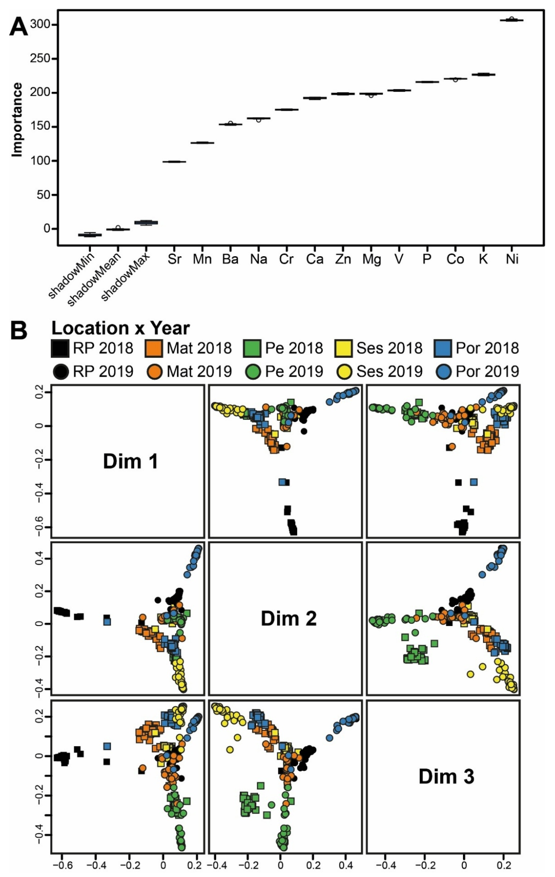
Random Forest provides robust classification in high-dimensional, noisy settings, and it can accommodate complex nonlinear relationships and interactions with minimal preprocessing. Random Forest offers stable performance with relatively modest tuning requirements [32]. Each Random Forest model was developed with enough classification trees to stabilize the classification error rate. The number of predictor variables sampled at each split was set to the square root of p, where p is the number of analyzed elements [32]. A double validation strategy was implemented for models of the points 1 and 3 described above. First, a train–test approach was used to enable validation with independent datasets. Second, an out-of-bag (OOB) approach was applied to better assess variable importance, allow visualization using the full dataset, and apply the 2018 samples as the reference model in model 2. For the train–test approach, the complete data matrix was randomly split using a 0.67:0.33 ratio, resulting in training and test datasets comprising 60 samples (20 replicates per location) and 30 samples (10 replicates per location), respectively. The Random Forest algorithm uses bootstrap resampling, and sample classification is evaluated with out-of-bag (OOB) estimation [32,33]. In contrast, the assessment of the influence of temporal variability on the confirmation of sampling locations (objective 2 above) was evaluated by the percentage of samples from 2019 correctly allocated using the 2018 reference model. The importance of the elements in model classification was performed using the Boruta feature selection algorithm using all samples [34,35]. Shadow variables are created through randomly permuted predictors that serve as a baseline for determining the relevance of real variables. Shadow Min, Shadow Mean, and Shadow Max correspond to the minimum, mean, and maximum importance values of these shadow variables, respectively. To better understand our results, it is essential to clarify that we considered only the seven elements that most effectively discriminated among the sampled locations. For each Random Forest classification using all samples, a multidimensional scaling (MDS) ordination based on proximity scores was generated to visualize similarities among samples.
PERMANOVA was performed using PRIMER v7 with the PERMANOVA+ add-on [36,37]. Random Forest classifications, boxplots, and Kruskal–Wallis tests were performed in the R software 4.5.1 [38] using the ‘randomForest’ [32], ‘ggplot2’ [39], and ‘agricolae’ [40] packages, respectively.

3. Results

3.1. Elemental Fingerprints

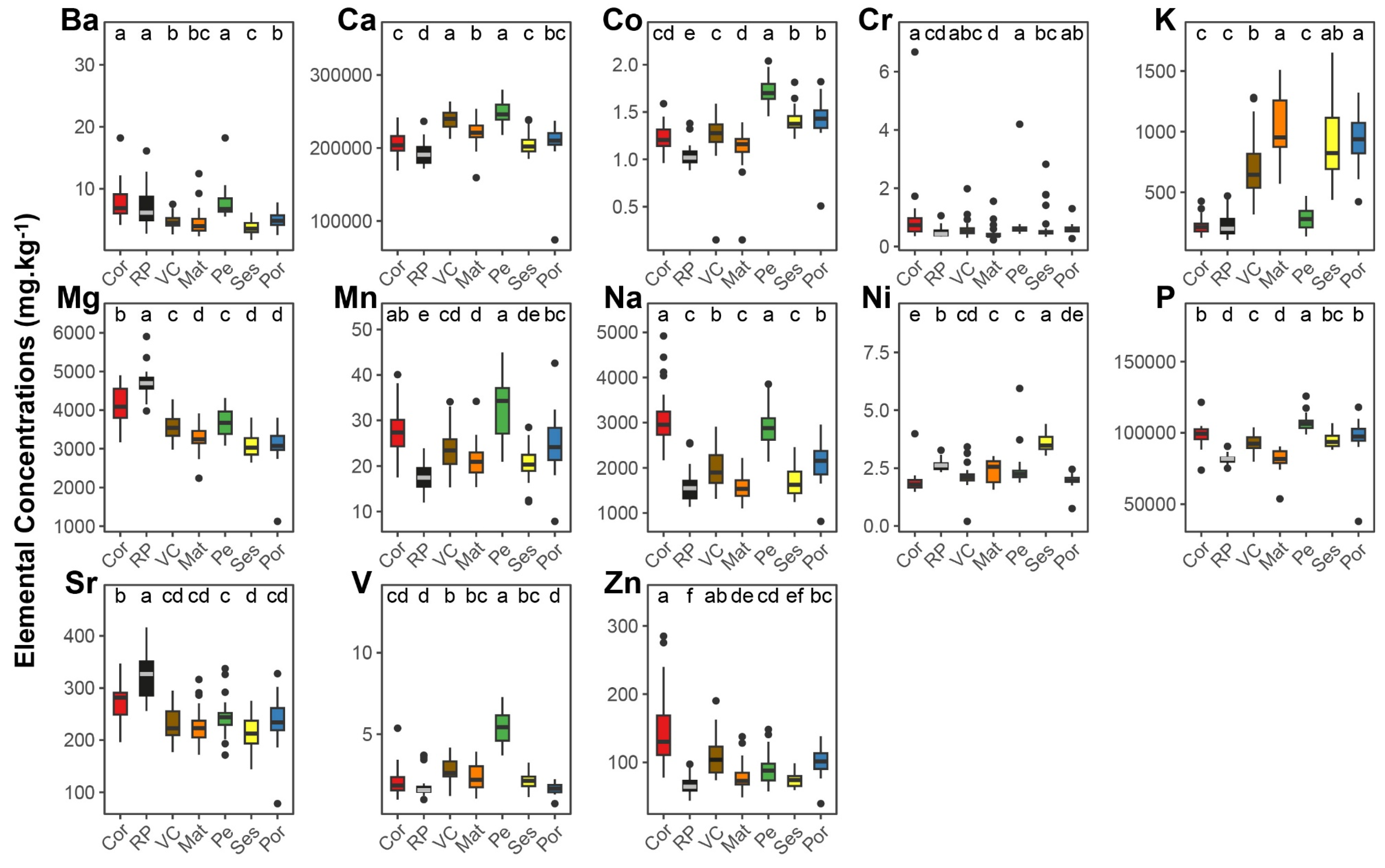
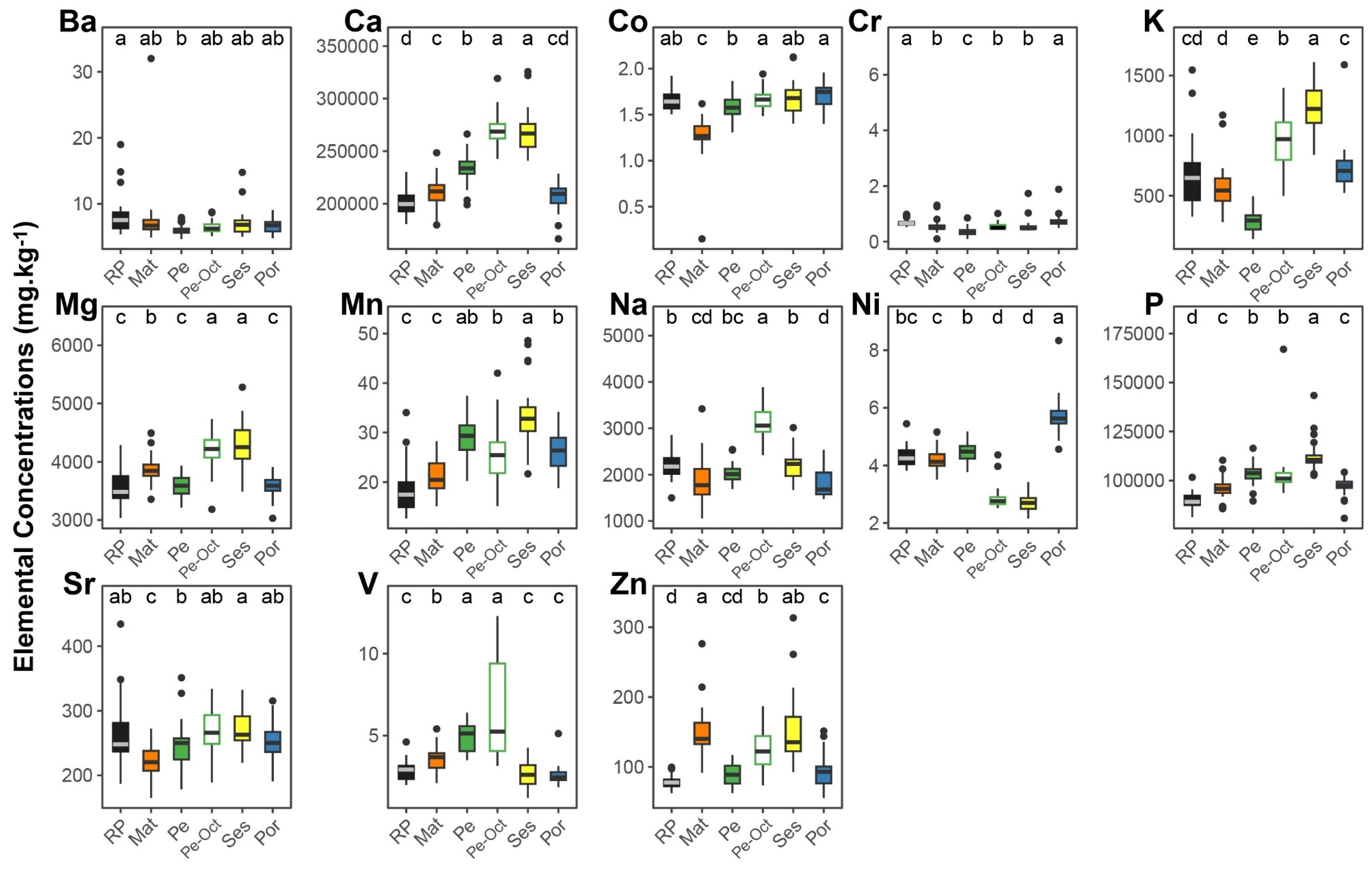
Thirteen elements (Ba, Ca, Co, Cr, K, Mg, Mn, Na, Ni, P, Sr, V, and Zn) consistently exhibited concentrations above detection limits (Figure 2 and Figure 3). The PERMANOVA revealed a highly significant interaction between location and time (p < 0.0001; see Table S1 in the Supplementary Material). The post hoc pairwise comparisons showed significant differences in EF across all locations within each time point (2018 and 2019) and across time points within each location (Table S1).
Several elements showed significant differences between locations (Figure 2). Although no clear spatial patterns were observed (e.g., consistent increases or decreases in elemental levels from North to South), some elements achieved the highest significant level at a single location (i.e., being significantly different from all other locations sampled). In 2018, the highest significant concentrations of Mg and Sr were observed in RP; of Co, P, and V in Pe; and of Ni in Ses (Figure 2). In 2019, Na and V displayed the highest significant concentrations in Pe (in Pe-Oct and Pe/Pe-Oct, respectively); of K and P in Ses; and of Ni in Por (Figure 3). Notably, V was the only element that consistently showed the highest significant levels at the same location (Pe) across both years (Figure 2 and Figure 3).

3.2. Confirmation of Geographic Origin

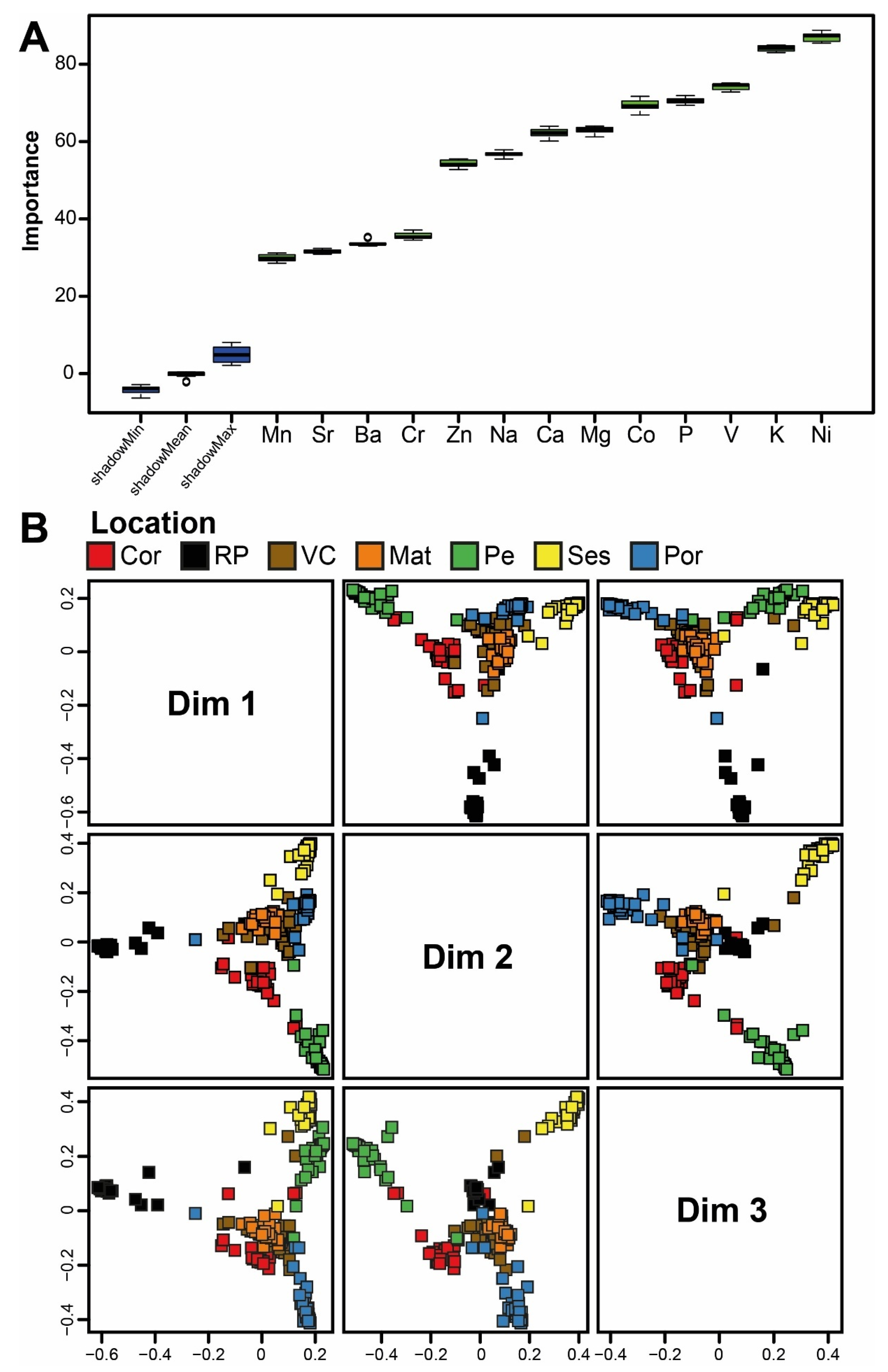
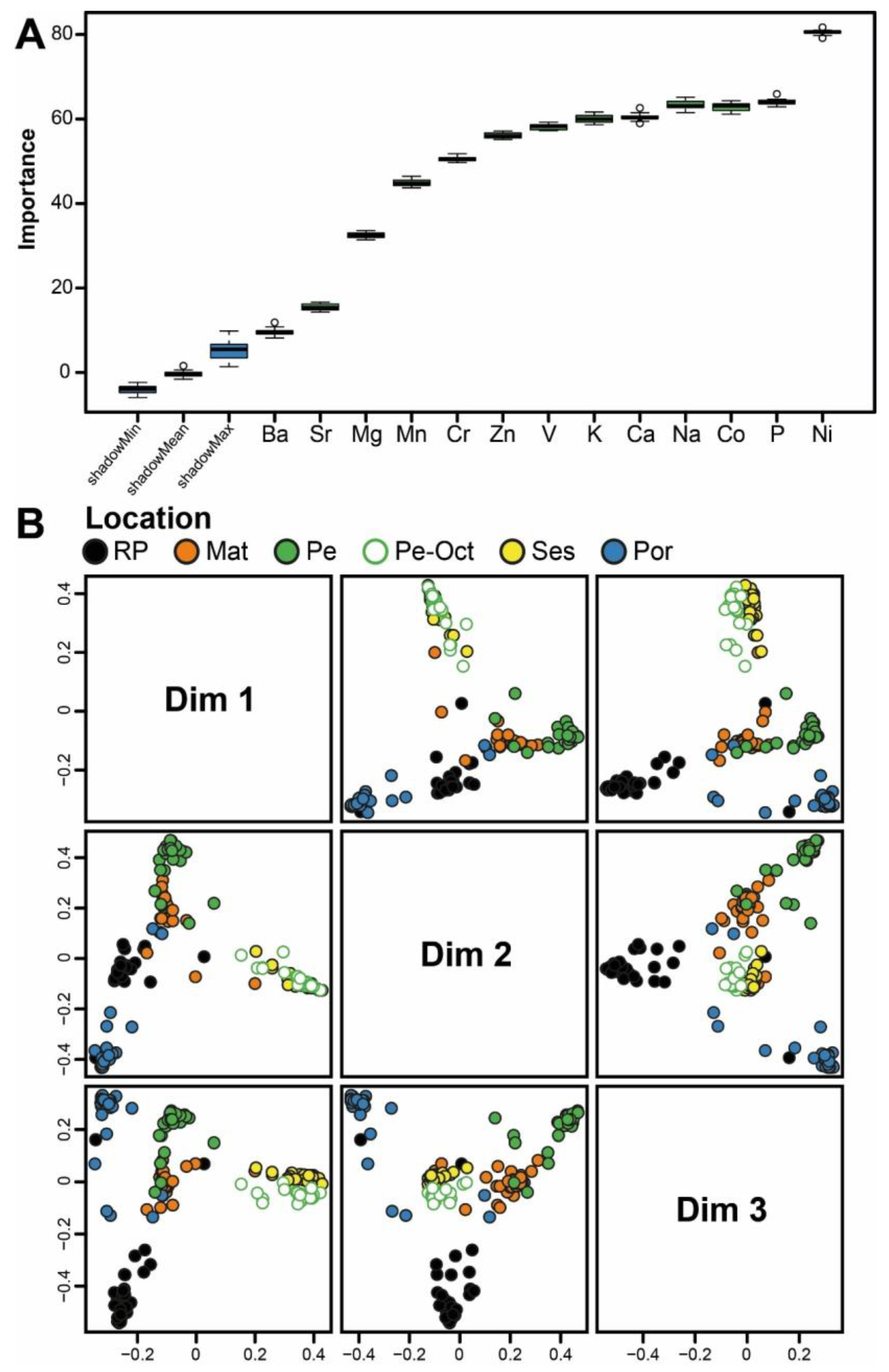
The Boruta selection algorithm identified all the elements analyzed as being important predictors in the 2018 and 2019 Random Forest classification models (Figure 4A and Figure 5A). In the 2018 model, the most relevant elements (in decreasing order of importance) were Ni, K, V, P, Co, Mg, and Ca (Figure 4A); in the 2019 model (also in decreasing order of importance), the most relevant elements were Ni, P, Co, Na, Ca, K, and V (Figure 5A). Notably, six of these elements (Ni, K, V, P, Co, and Ca) were among the most important in both models.
Both Random Forest models (2018 and 2019) achieved high classification accuracy, correctly assigning 97.1 and 95.7% of samples to their respective sampling locations in 2018 and 95.7 and 95.6% in 2019, for test dataset and out-of-bag (all samples) approach, respectively (Table S1 and Table 1). For all locations, at least 90% of samples were correctly classified (Table 1). In the 2018 model, samples from Mat were classified with 100% accuracy, while those from VC had the lowest accuracy (90%). In the 2019 model, all samples from Pe-Oct, Ses, and Por were correctly classified (100%), while samples from RP and Pe exhibited the lowest accuracy (93.3%; Table 1). Importantly, the two Pe measurements in 2019 (Pe and Pe-Oct) were clearly differentiated. These high classification accuracies were supported by the distinct clustering patterns of the different landing locations displayed in the MDS plots of proximity scores (Figure 4B and Figure 5B). While most locations formed well-defined clusters in at least one MDS plot, VC and Mat in 2018 were exceptions, showing partial overlap across all plots (Figure 4B and Figure 5B).
Applying the 2018 Random Forest model to the 2019 dataset revealed a pronounced effect of temporal variability on model performance. Classification accuracy decreased substantially, with only 24.4% of samples being correctly assigned to their original locations (Table 2). Correct classifications were limited to Pe (80%) and Pe-Oct (66%), while all samples from RP, Mat, Ses, and Por were misclassified (Table 2).

3.3. Confirmation of Sampling Time

The Boruta selection algorithm identified all elements analyzed as relevant predictors for the Random Forest model developed to confirm sampling time (Figure 6A). The most important elements (in decreasing order of importance) were Ni, K, Co, P, V, Mg, and Zn (Figure 6A). The model achieved high overall accuracy, correctly assigning 95 and 95.3% of the samples to their respective origins (location × year) for test dataset and out-of-bag (all samples) approach, respectively (Table S2 and Table 3). Classification accuracies ranged from 86.7% (Por 2019) to 100% (Mat 2018, Pe 2018, and Ses 2019). The MDS ordination of Random Forest proximity scores (Figure 6B) further supports the model’s performance by showing clear clustering of samples by location × time. Despite the considerable number of origins (n = 10), the MDS plots displayed well-defined, distinct origins.

4. Discussion

The global decline in fish stocks driven by overexploitation, pollution, and climate change have prompted stricter fisheries management worldwide [1,41]. The S. pilchardus fishery in Portugal and Spain is a good example of this global shift. The implementation of catch limits, seasonal closures, and selective spatial restrictions has been paramount in the recovery of the stocks of this vital fishing resource [5,9,42]. Within this framework, effective traceability systems are essential for ensuring seafood authenticity, protecting consumers, and supporting sustainable fisheries [17]. Analytical approaches based on biochemical signatures of fish, particularly EF, strengthen these systems by providing reliable indicators of seafood origin [22,25]. In this context, this study evaluates the potential of EF in S. pilchardus scales to confirm the location and time of capture of this small pelagic fish to assess the influence of EF temporal variability on geographic traceability.
Previous studies have observed geographic variation in the EF of S. pilchardus muscle, e.g., [43], as recorded in the present study for the EF of its scales. Such differences are unlikely to reflect genetic variation, as S. pilchardus from Galicia and Portugal are known to belong to the same metapopulation and exhibit low genetic differentiation [44,45]. Instead, these patterns presumably result from spatial variability in seawater elemental inputs [46,47] and circulation dynamics [48], which shape local seawater chemistry [49,50] and influence element uptake by marine organisms during growth. Among the elements analyzed, Ni, K, V, P, and Co were the most relevant to the Random Forest models, consistent with previous findings for biomineralized structures of marine organisms [51,52,53]. Among the most important elements, only Ni, V, and P exhibited significantly higher concentrations at one location in both years, although not necessarily in the same location. The elevated Ni levels recorded in the scales of S. pilchardus at the southernmost locations (Ses in 2018 and Por in 2019) are consistent with Ni-rich topsoil in southern Portugal [54]. In turn, the high concentrations of P recorded in specimens from Pe in 2018 and Ses in 2019 mirror those observed in gooseneck barnacles Pollicipes pollicipes capitula collected from those same regions and time periods [52]. These high P concentrations may be linked to the elevated phosphate levels recorded in seawater offshore the Tagus estuary [50], which lies between Pe and Ses. These southward shifts in Ni and P concentrations—from Ses to Por and from Pe to Ses, respectively—between 2018 and 2019 suggest that coastal circulation most likely influenced the distribution of these elements in that direction. Finally, the higher V concentrations recorded in specimens captured near Pe in both years likely reflect historical industrial and maritime emissions in the area [55], including those from shipping emissions and fuel combustion [56,57]. Collectively, these results underscore the EF of fish scales as a sensitive indicator of environmental and anthropogenic variability in coastal ecosystems.
The high classification accuracies achieved by the Random Forest models (95.7% for 2018 and 95.6% for 2019) highlight the strong potential of EF in fish scales to confirm the geographic origin of small pelagic marine fish. These results are comparable to the accuracy reported for identifying the hatchery of Atlantic salmon smolts using the EF of their scales [95.8%; [28]]. The methods developed here can support the valorization of S. pilchardus from premium regions by authenticating local sardines and distinguishing them from imports, thereby reinforcing consumers’ trust and willingness to pay for authenticated locally captured seafood [58]. Notably, samples from the same harbor (Pe) in early summer and October of 2019 were clearly differentiated. Because scales record elemental information during fish development, and given the short sampling interval, the differentiation observed likely reflects environmental variability experienced by different shoals during growth, consistent with this species’ high mobility [59].
Regular model updates are necessary to account for temporal variation, which can be resource-intensive. As such, to successfully implement EF-based traceability tools, one must enhance their cost-efficiency, but without compromising accuracy. The sharp decline in classification accuracy (24.4%) observed when samples from 2019 were classified with the 2018 reference model indicates that interannual shifts in the EF of S. pilchardus scales compromise geographic traceability and hinder the optimization of this method. This result aligns with the accuracies reported for goose barnacles P. pollicipes [5–31.4%; [52]], although it is lower than the results obtained for Manila clams Ruditapes philippinarum [63.3–85.6%; [60]] using comparable methods. Nevertheless, localized applications remain possible, as evidenced by the relatively high percentage of correct assignments recorded for S. pilchardus sampled in Pe during 2019 (80% and 66% for Pe and Pe-Oct, respectively).
While the temporal variability of EF limits long-term stability of the models, it adds an important dimension to seafood traceability. The ability to classify samples by location and time with an accuracy of 95.3% discloses the potential that the EF of fish scales holds for temporal traceability. Similar temporal discrimination has been reported for goose barnacles P. pollicipes [52], Manila clams R. philippinarum [60], king scallops Pecten maximus [61], and blue mussels Mytilus edulis [62]. However, to the best of our knowledge, this is the first report of such an application that has been reported for fish. This ability is particularly relevant for frozen sardines, as it makes it possible to verify the compliance with fishing closures and freezing duration, as well as prevent the mislabeling of frozen specimens as “freshly caught”.
Integrating geographic and temporal traceability provides a robust framework for seafood authentication and fisheries management. Indeed, EF-based methods can verify legal catches, enforce closures, and expose mislabeling. Traceability tools based on the EF of fish scales offer a practical, non-destructive, and scientifically robust approach that can be incorporated into monitoring and certification frameworks. Ultimately, this approach can help to promote the sustainable exploitation of fishing stocks and guarantee that the recovery of emblematic fishing resources, such as the European sardine S. pilchardus, is accompanied by reliable, transparent and traceable supply chains.

5. Conclusions

This study demonstrated that EF of S. pilchardus scales exhibit distinct spatial and temporal variability, enabling geographic and temporal traceability, while interannual shifts in EF reduce model accuracy, underscoring the need for regular updates to maintain reliability. Despite this limitation, the approach addressed in the present study contributed to the development of a practical, non-destructive, and scientifically robust method for the authentication and certification of S. pilchardus. The practical applications of the methodologies developed in this study can include the discrimination of S. pilchardus specimens captured in the Atlantic from conspecifics imported from the Mediterranean and readily applying this approach to other commercially important fish species. These methodologies enhance consumers trust, foster more sustainable fishery practices, and increase the value of this culturally and economically important bioresource. Future research should focus on improving the cost-efficiency and long-term robustness of these tools, namely by integrating complementary markers (e.g., fatty acid profiles or stable isotopes) directly from fish tissues (e.g., scales or muscle) or DNA analysis of bacterial communities associated with some of those fish tissues (e.g., gut or gills). Additionally, further evaluating temporal traceability across multiple timescales will be essential to refine and expand spatial and temporal traceability models.

Supplementary Materials

The following supporting information can be downloaded at: https://www.mdpi.com/article/10.3390/fishes11030138/s1. Table S1: Results of PERMANOVA main tests and pairwise comparisons of the elemental fingerprints of Sardina pilchardus scales collected from fishing harbors in Galicia (Spain) and mainland Portugal along the NW, W, and SW Iberian coast. Malpica—A Coruña (Cor), Bueu—Ría de Pontevedra (RP), Viana do Castelo (VC), Matosinhos (Mat), Peniche (Pe), Peniche October (Pe-Oct), Sesimbra (Ses), and Portimão (Por). Significant differences at p < 0.05; Table S2: Confusion matrices of the Random Forest classifications based on the elemental fingerprints of European sardine Sardina pilchardus scales collected from fishing harbors in Galicia (Spain) and mainland Portugal along the NW, W, and SW Iberian coast. Malpica—A Coruña (Cor), Bueu—Ría de Pontevedra (RP), Viana do Castelo (VC), Matosinhos (Mat), Peniche (Pe), Peniche—October (Pe-Oct), Sesimbra (Ses), and Portimão (Por). Evaluation performed with an independent test dataset; Table S3: Confusion matrix of the Random Forests classifications based on the elemental fingerprints of European sardine Sardina pilchardus scales collected in 2018 and 2019 from five fishing harbors along the Atlantic NW, W, and SW Iberian coast. Bueu—Ría de Pontevedra 2018 (RP 2018), Bueu—Ría de Pontevedra 2019 (RP 2019), Matosinhos 2018 (Mat 2018), Matosinhos 2019 (Mat 2019), Peniche 2018 (Pe 2018), Peniche 2019 (Pe 2019), Sesimbra 2018 (Ses 2018), Sesimbra 2019 (Ses 2019), Portimão 2018 (Por 2018), and Portimão 2019 (Por 2019). Evaluation performed with an independent test dataset.

Author Contributions

R.M.: Data curation, Formal analysis, Methodology, Writing—original draft, Writing—review and editing. C.P.: Supervision, Methodology, Data curation, Writing—review and editing. S.D.: Resources, Writing—review and editing. E.F.d.S.: Writing—review and editing. R.C.: Conceptualization, Formal analysis, Project administration, Supervision, Writing—review and editing. F.R.: Conceptualization, Data curation, Formal analysis, Methodology, Writing—review and editing. All authors have read and agreed to the published version of the manuscript.

Funding

This work was financially supported by the project CITAQUA “Desenvolvimento do Projeto de Reforço do Polo de Aveiro (H4)”, framed within Measure 10 of Investment TC-C10-i01—Hub Azul-Rede de Infraestruturas para a Economia Azul, financed by the Recovery and Resilience Plan (PRR) and supported by Fundo Azul of the Portuguese Government. National funds funded this work through FCT—Fundação para a Ciência e a Tecnologia I.P., under the project CESAM-Centro de Estudos do Ambiente e do Mar, references UID/50017/2025 (doi.org/10.54499/UID/50017/2025) and LA/P/0094/2020 (doi.org/10.54499/LA/P/0094/2020). The authors also acknowledge the project “Impacto e Consolidação em I&DT da Unidade de Investigação Química Orgânica, Produtos Naturais e Agroalimentares em áreas Agroalimentares e afins ICT_2009_02_005_2034” for financing the ICP-MS. The authors would like to thank the crew of the ‘Afrodite’ fishing vessel, with special thanks to Luis Santana and José Maria Ricardo “Zézito”, for their valuable assistance during the sampling campaigns.

Institutional Review Board Statement

All specimens were obtained directly from landing piers through trusted local fishermen, who confirmed that the sardines were caught in coastal waters adjacent to each harbor. The fish were captured, stored on board under refrigeration, and were already dead upon landing. Therefore, ethical considerations related to animal experimentation and welfare do not apply to the present study.

Data Availability Statement

The original contributions presented in this study are included in the article. Further inquiries can be directed to the corresponding author.

Conflicts of Interest

The authors declare that there are no conflicts of interest regarding the publication of this article.

References

  1. FAO. The State of World Fisheries and Aquaculture 2024: Blue Transformation in Action; FAO: Rome, Italy, 2024; ISBN 978-92-5-138763-4. [Google Scholar]
  2. Tacon, A.G.J.; Levy, J.; Coelho, R.; Machado, T.M.; Neiva, C.R.P.; Lemos, D.E.L. Fish for Health: Role of Fish in Global Food and Animal Protein Supply. Rev. Fish. Sci. Aquac. 2025, 33, 319–333. [Google Scholar] [CrossRef] [Scilit]
  3. UN. Transforming Our World: The 2030 Agenda for Sustainable Development; UN: New York, NY, USA, 2016. [Google Scholar]
  4. EUMOFA. The EU Fish Market. Highlights the EU in the World Market Supply Consumption Import—Export Landings in the EU Aquaculture; EUMOFA: Luxembourg, 2024; ISBN 978-92-68-22586-8. [Google Scholar]
  5. MAR and MAPAMA. Multiannual Management Plan for the Iberian Sardine (2021–2026); MAR and MAPAMA: London, UK, 2020; Available online: https://www.dgrm.pt/documents/20143/46478/PGSARDINHA2021-2026.pdf/d36a1df9-7353-32a4-a06e-c72852e73cb0 (accessed on 16 September 2025).
  6. Monteiro, P.V. The Purse Seine Fishing of Sardine in Portuguese Waters: A Difficult Compromise Between Fish Stock Sustainability and Fishing Effort. Rev. Fish. Sci. Aquac. 2017, 25, 218–229. [Google Scholar] [CrossRef] [Scilit]
  7. INE. Estatísticas Da Pesca—2024. Available online: https://www.ine.pt/xportal/xmain?xpid=INE&xpgid=ine_publicacoes&PUBLICACOESpub_boui=66198697&PUBLICACOESmodo=2 (accessed on 16 September 2025).
  8. Pesca de Galicia. Anuario de Pesca 2024, Especies Máis Importantes En Importe (€). Available online: https://www.pescadegalicia.gal/Publicaciones/AnuarioPesca2024/Informes/3.1.4.html (accessed on 16 September 2025).
  9. ICES. Working Group on Southern Horse Mackerel, Anchovy and Sardine (WGHANSA); ICES Scientific Reports, 6:46; ICES: Copenhagen, Denmark, 2024. [Google Scholar]
  10. Shockites, Z.E. Sustainability and the Sea: Environmental Policy and the Portuguese Canned Fish Sector. J. Glob. Bus. Community 2025, 16, 1–22. [Google Scholar] [CrossRef] [Scilit]
  11. Dominguez-Martinez, R.M.; Klein, C.J.; Blanchard, J.L.; Farmery, A.; Kuempel, C.D.; Roberson, L.; Spillias, S.; Cottrell, R.S. Seafood Sustainability Challenges for Import-Dependent Nations. Rev. Fish. Sci. Aquac. 2025, 1–16. [Google Scholar] [CrossRef] [Scilit]
  12. Karunasagar, I. Issues in International Trade of Seafood. In Aquatic Animal Health Management; Kooloth Valappil, R., Karunasagar, I., Karunasagar, I., Eds.; Springer: Singapore, 2025; pp. 881–897. [Google Scholar]
  13. EC. Council Regulation (EC) No 104/2000 of 17 December 1999 on the Common Organisation of the Markets in Fishery and Aquaculture Products. Off. J. Eur. Communities 2000, 17, 22–52. [Google Scholar]
  14. EC. Commission Regulation (EC) No 2065/2001 of 22 October 2001 Laying Down Detailed Rules for the Application of Council Regulation (EC) No 104/2000 as Regards Informing Consumers about Fishery and Aquaculture Products (Text with EEA Relevance). Off. J. Eur. Communities 2001, 278, 6–8. [Google Scholar]
  15. EC. Regulation (EC) No 178/2002 of the European Parliament and of the Council of 28 January 2002 Laying Down the General Principles and Requirements of Food Law, Establishing the European Food Safety Authority and Laying down Procedures in Matters of Food Safety. Off. J. Eur. Communities 2002, 31, 1–24. [Google Scholar]
  16. EC. Council Regulation (EC) No 1224/2009 of 20 November 2009 Establishing a Community Control System for Ensuring Compliance with the Rules of the Common Fisheries Policy, Amending Regulations (EC) No 847/96, (EC) No 2371/2002, (EC) No 811/2004, (EC) No 768/2005, (EC) No 2115/2005, (EC) No 2166/2005, (EC) No 388/2006, (EC) No 509/2007, (EC) No 676/2007, (EC) No 1098/2007, (EC) No 1300/2008, (EC) No 1342/2008 and repealing Regulations (EEC) No 2847/93, (EC) No 1627/94 and (EC) No 1966/2006. Off. J. Eur. Union 2009, 343, 1–50. [Google Scholar]
  17. EC. A Farm to Fork Strategy for a Fair, Healthy and Environmentally-Friendly Food; European Union: Brussels, Belgium, 2020. [Google Scholar]
  18. EU. Regulation (EU) No 1379/2013 of the European Parliament and of the Council of 11 December 2013 on the Common Organisation of the Markets in Fishery and Aquaculture Products, Amending Council Regulations (EC) No 1184/2006 and (EC) No 1224/2009 and Repealing Council Regulation (EC) No 104/2000. Off. J. Eur. Union 2013, 354, 1–21. [Google Scholar]
  19. Kroetz, K.; Luque, G.M.; Gephart, J.A.; Jardine, S.L.; Lee, P.; Moore, K.C.; Cole, C.; Steinkruger, A.; Josh Donlan, C. Consequences of Seafood Mislabeling for Marine Populations and Fisheries Management. Proc. Natl. Acad. Sci. USA 2020, 117, 30318–30323. [Google Scholar] [CrossRef] [Scilit]
  20. Leal, M.C.; Pimentel, T.; Ricardo, F.; Rosa, R.; Calado, R. Seafood Traceability: Current Needs, Available Tools, and Biotechnological Challenges for Origin Certification. Trends Biotechnol. 2015, 33, 331–336. [Google Scholar] [CrossRef] [Scilit]
  21. Gleadall, I.G.; Moustahfid, H.; Sauer, W.H.H.; Ababouch, L. Towards Global Traceability for Sustainable Cephalopod Seafood. Mar. Biol. 2024, 171, 44. [Google Scholar] [CrossRef] [Scilit]
  22. Gopi, K.; Mazumder, D.; Sammut, J.; Saintilan, N. Determining the Provenance and Authenticity of Seafood: A Review of Current Methodologies. Trends Food Sci. Technol. 2019, 91, 294–304. [Google Scholar] [CrossRef] [Scilit]
  23. Santos, A.; Ricardo, F.; Domingues, M.R.M.; Patinha, C.; Calado, R. Current Trends in the Traceability of Geographic Origin and Detection of Species-Mislabeling in Marine Bivalves. Food Control 2023, 152, 109840. [Google Scholar] [CrossRef] [Scilit]
  24. Parvez, M.S.; Hoque, M.I.; Siddique, M.N.M.; Rahman, M.M.; Baranyai, E.; Sajtos, Z.; Döncző, B.; Aib, H.; Kader, M.A.; Simon, E.; et al. Elemental Analysis in the Scales of Commercially Important Coastal Fishes and Their Connections with Fish Feeding Habits and Habitats. Front. Mar. Sci. 2025, 12, 1546313. [Google Scholar] [CrossRef] [Scilit]
  25. Varrà, M.O.; Ghidini, S.; Husáková, L.; Ianieri, A.; Zanardi, E. Advances in Troubleshooting Fish and Seafood Authentication by Inorganic Elemental Composition. Foods 2021, 10, 270. [Google Scholar] [CrossRef] [Scilit] [PubMed]
  26. Duarte, B.; Duarte, I.; Caçador, I.; Reis-Santos, P.; Vasconcelos, R.P.; Gameiro, C.; Tanner, S.E.; Fonseca, V.F. Elemental Fingerprinting of Thornback Ray (Raja clavata) Muscle Tissue as a Tracer for Provenance and Food Safety Assessment. Food Control 2021, 133, 108592. [Google Scholar] [CrossRef] [Scilit]
  27. Arai, T.; Kimura, S. Spatiotemporal Variability of Trace Elements Fingerprints in Otoliths of Japanese Eel (Anguilla japonica) and Its Use in Tracing Geographic Origin. Biology 2022, 11, 1733. [Google Scholar] [CrossRef] [Scilit] [PubMed]
  28. Flem, B.; Moen, V.; Finne, T.E.; Viljugrein, H.; Kristoffersen, A.B. Trace Element Composition of Smolt Scales from Atlantic Salmon (Salmo salar L.), Geographic Variation between Hatcheries. Fish. Res. 2017, 190, 183–196. [Google Scholar] [CrossRef] [Scilit]
  29. Basilone, G.; Ferreri, R.; Bonanno, A.; Genovese, S.; Barra, M.; Aronica, S. Age and Growth of European Sardine (Sardina pilchardus) in the Central Mediterranean Sea: Implication for Stock Assessment. Fishes 2023, 8, 202. [Google Scholar] [CrossRef] [Scilit]
  30. Reis-Santos, P.; Gillanders, B.M.; Sturrock, A.M.; Izzo, C.; Oxman, D.S.; Lueders-Dumont, J.A.; Hüssy, K.; Tanner, S.E.; Rogers, T.; Doubleday, Z.A.; et al. Reading the Biomineralized Book of Life: Expanding Otolith Biogeochemical Research and Applications for Fisheries and Ecosystem-Based Management. Rev. Fish Biol. Fish. 2023, 33, 411–449. [Google Scholar] [CrossRef] [Scilit]
  31. EC. Council Regulation (EC) No 2406/96 of 26 November 1996 Laying down Common Marketing Standards for Certain Fishery Products. Off. J. Eur. Communities 1996, 334, 1–15. [Google Scholar]
  32. Breiman, L. Random Forests. Mach. Learn. 2001, 45, 5–32. [Google Scholar] [CrossRef] [Scilit]
  33. Liaw, A.; Wiener, M. Classification and Regression by RandomForest. R News 2002, 2, 18–22. [Google Scholar]
  34. Kursa, M.B.; Rudnicki, W.R. Feature Selection with the Boruta Package. J. Stat. Softw. 2010, 36, 1–13. [Google Scholar] [CrossRef] [Scilit]
  35. Kursa, M.B.; Rudnicki, W.R. ‘Boruta’ 7.0.0: Wrapper Algorithm for All Relevant Feature Selection; CRAN, 2020; Available online: https://cran.r-project.org/web/packages/Boruta/Boruta.pdf (accessed on 23 September 2025).
  36. Anderson, M.J.; Gorley, R.N.; Clarke, K.R. PERMANOVA+ for PRIMER: Guide to Software and Statistical Methods; PRIMER-E Ltd.: Plymouth, UK, 2008. [Google Scholar]
  37. Clarke, K.R.; Gorley, R.N. PRIMER v7: User Manual/Tutorial; PRIMER-E: Plymouth, UK, 2015. [Google Scholar]
  38. R Core Team. R 4.5.1; A Language and Environment for Statistical Computing. 2025. Available online: https://www.r-project.org/ (accessed on 23 September 2025).
  39. Wickham, H. Ggplot2: Create Elegant Data Visualisations Using the Grammar of Graphics; CRAN, 2021; Available online: https://cran.r-project.org/web/packages/ggplot2/ggplot2.pdf (accessed on 23 September 2025).
  40. Mendiburu, F. “agricolae” 1.3-5: Statistical Procedures for Agricultural Research; CRAN, 2021; Available online: https://cran.r-project.org/web/packages/agricolae/agricolae.pdf (accessed on 23 September 2025).
  41. Hilborn, R.; Hively, D.J.; Loke, N.B.; de Moor, C.L.; Kurota, H.; Kathena, J.N.; Mace, P.M.; Minto, C.; Parma, A.M.; Quiroz, J.C.; et al. Global Status of Groundfish Stocks. Fish Fish. 2021, 22, 911–928. [Google Scholar] [CrossRef] [Scilit]
  42. MSC. Iberian Sardine Regains MSC Certification: A Milestone for Sustainable Fishing in Spain and Portugal. Available online: https://www.msc.org/media-centre/press-releases/press-release/iberian-sardine-regains-msc-certification--a-milestone-for-sustainable-fishing-in-spain-and-portugal?utm_source=chatgpt.com (accessed on 6 October 2025).
  43. Lozano-Bilbao, E.; Jurado-Ruzafa, A.; Hardisson, A.; Lorenzo, J.M.; González, J.A.; González-Weller, D.; Paz, S.; Rubio, C.; Techetach, M.; Guillén, F.; et al. Tracing Metals in Mediterranean and Atlantic Sardina pilchardus: Unveiling Impacts on Food Safety. Sci. Total Environ. 2025, 958, 178042. [Google Scholar] [CrossRef] [Scilit]
  44. da Fonseca, R.R.; Campos, P.F.; Rey-Iglesia, A.; Barroso, G.V.; Bergeron, L.A.; Nande, M.; Tuya, F.; Abidli, S.; Pérez, M.; Riveiro, I.; et al. Population Genomics Reveals the Underlying Structure of the Small Pelagic European Sardine and Suggests Low Connectivity within Macaronesia. Genes 2024, 15, 170. [Google Scholar] [CrossRef] [Scilit]
  45. Silva, A.; Garrido, S.; Ibaibarriaga, L.; Pawlowski, L.; Riveiro, I.; Marques, V.; Ramos, F.; Duhamel, E.; Iglesias, M.; Bryère, P.; et al. Adult-Mediated Connectivity and Spatial Population Structure of Sardine in the Bay of Biscay and Iberian Coast. Deep Sea Res. Part II Top. Stud. Oceanogr. 2019, 159, 62–74. [Google Scholar] [CrossRef] [Scilit]
  46. Richir, J.; Gobert, S. Trace Elements in Marine Environments: Occurrence, Threats and Monitoring with Special Focus on the Costal Mediterranean. J. Environ. Anal. Toxicol. 2016, 6, 1–19. [Google Scholar] [CrossRef]
  47. Sánchez-Quiles, D.; Marbà, N.; Tovar-Sánchez, A. Trace Metal Accumulation in Marine Macrophytes: Hotspots of Coastal Contamination Worldwide. Sci. Total Environ. 2017, 576, 520–527. [Google Scholar] [CrossRef] [Scilit]
  48. Costa, T.C.; Pereira, L.T.; Marta-Almeida, M.; Guedes Soares, C. Mapping of Currents off the Northwestern Iberian Coast with the Regional Ocean Modelling System. J. Oper. Oceanogr. 2020, 13, 71–83. [Google Scholar] [CrossRef] [Scilit]
  49. Mellett, T.; Buck, K.N. Spatial and Temporal Variability of Trace Metals (Fe, Cu, Mn, Zn, Co, Ni, Cd, Pb), Iron and Copper Speciation, and Electroactive Fe-Binding Humic Substances in Surface Waters of the Eastern Gulf of Mexico. Mar. Chem. 2020, 227, 103891. [Google Scholar] [CrossRef] [Scilit]
  50. Santos-Echeandía, J.; Caetano, M.; Brito, P.; Canario, J.; Vale, C. The Relevance of Defining Trace Metal Baselines in Coastal Waters at a Regional Scale: The Case of the Portuguese Coast (SW Europe). Mar. Environ. Res. 2012, 79, 86–99. [Google Scholar] [CrossRef] [Scilit] [PubMed]
  51. Duarte, B.; Reis-santos, P.; Tanner, S.E.; Mamede, R.; Duarte, I.A.; Caçador, I.; Vasconcelos, R.P.; Gameiro, C.; Rosa, R.; Fonseca, V.F. Elemental and Spectral Chemometric Analyses of Octopus vulgaris Beaks as Reliable Markers of Capture Location. J. Food Sci. 2023, 88, 1349–1364. [Google Scholar] [CrossRef] [Scilit]
  52. Mamede, R.; Patinha, C.; Marques, S.C.; Díaz, S.; Aguión, A.; Leandro, S.M.; Calado, R.; Ricardo, F. Spatio-Temporal Variability of Elemental Fingerprints of Goose Barnacles (Pollicipes pollicipes) Capitula and Its Relevance to Fight Poaching through Traceability. Ecol. Indic. 2025, 178, 113913. [Google Scholar] [CrossRef] [Scilit]
  53. Ricardo, F.; Lopes, M.L.; Mamede, R.; Domingues, M.R.; Ferreira da Silva, E.; Patinha, C.; Calado, R. Combined Use of Fatty Acid Profiles and Elemental Fingerprints to Trace the Geographic Origin of Live Baits for Sports Fishing: The Solitary Tube Worm (Diopatra neapolitana, Annelida, Onuphidae) as a Case Study. Animals 2024, 14, 1361. [Google Scholar] [CrossRef] [Scilit]
  54. Inácio, M.; Pereira, V.; Pinto, M. The Soil Geochemical Atlas of Portugal: Overview and Applications. J. Geochem. Explor. 2008, 98, 22–33. [Google Scholar] [CrossRef] [Scilit]
  55. Moniz, A.; Kovács, I.; Vicente, D.; Ramos, A. Fisheries Development and Fisheries Dependent Communities in Portugal: Socio-Economic Change and Strategic Planning. In Fisheries Dependent Regions; Symes, D., Ed.; Fishing New Books: London, UK, 2000; pp. 143–153. [Google Scholar]
  56. Tambat, V.S.; Patel, A.K.; Singhania, R.R.; Chen, C.W.; Dong, C. Marine Vanadium Pollution: Sources, Ecological Impacts and Cutting-Edge Mitigation Strategies. Mar. Pollut. Bull. 2024, 209, 117199. [Google Scholar] [CrossRef] [Scilit]
  57. Tulcan, R.X.S.; Ouyang, W.; Lin, C.; He, M.; Wang, B. Vanadium Pollution and Health Risks in Marine Ecosystems: Anthropogenic Sources over Natural Contributions. Water Res. 2021, 207, 117838. [Google Scholar] [CrossRef] [Scilit]
  58. Fonner, R.; Sylvia, G. Willingness to Pay for Multiple Seafood Labels in a Niche Market. Mar. Resour. Econ. 2015, 30, 51–70. [Google Scholar] [CrossRef] [Scilit]
  59. Carrera, P.; Porteiro, C. Stock Dynamic of the Iberian Sardine (Sardina pilchardus, W.) and Its Implication on the Fishery off Galicia (NW Spain). Sci. Mar. 2003, 67, 245–258. [Google Scholar] [CrossRef] [Scilit]
  60. Santos, A.; Ricardo, F.; Mamede, R.; Díaz, S.; Patinha, C.; Calado, R. Spatio-Temporal Variation of Elemental Fingerprints of Ruditapes philippinarum Shells and Its Influence on the Confirmation of Harvesting Location and Time. Estuar. Coast. Shelf. Sci. 2025, 324, 109444. [Google Scholar] [CrossRef] [Scilit]
  61. Morrison, L.; Bennion, M.; Gill, S.; Graham, C.T. Spatio-Temporal Trace Element Fingerprinting of King Scallops (Pecten maximus) Reveals Harvesting Period and Location. Sci. Total Environ. 2019, 697, 134121. [Google Scholar] [CrossRef] [Scilit]
  62. Bennion, M.; Morrison, L.; Shelley, R.; Graham, C. Trace Elemental Fingerprinting of Shells and Soft Tissues Can Identify the Time of Blue Mussel (Mytilus edulis) Harvesting. Food Control 2021, 121, 107515. [Google Scholar] [CrossRef] [Scilit]
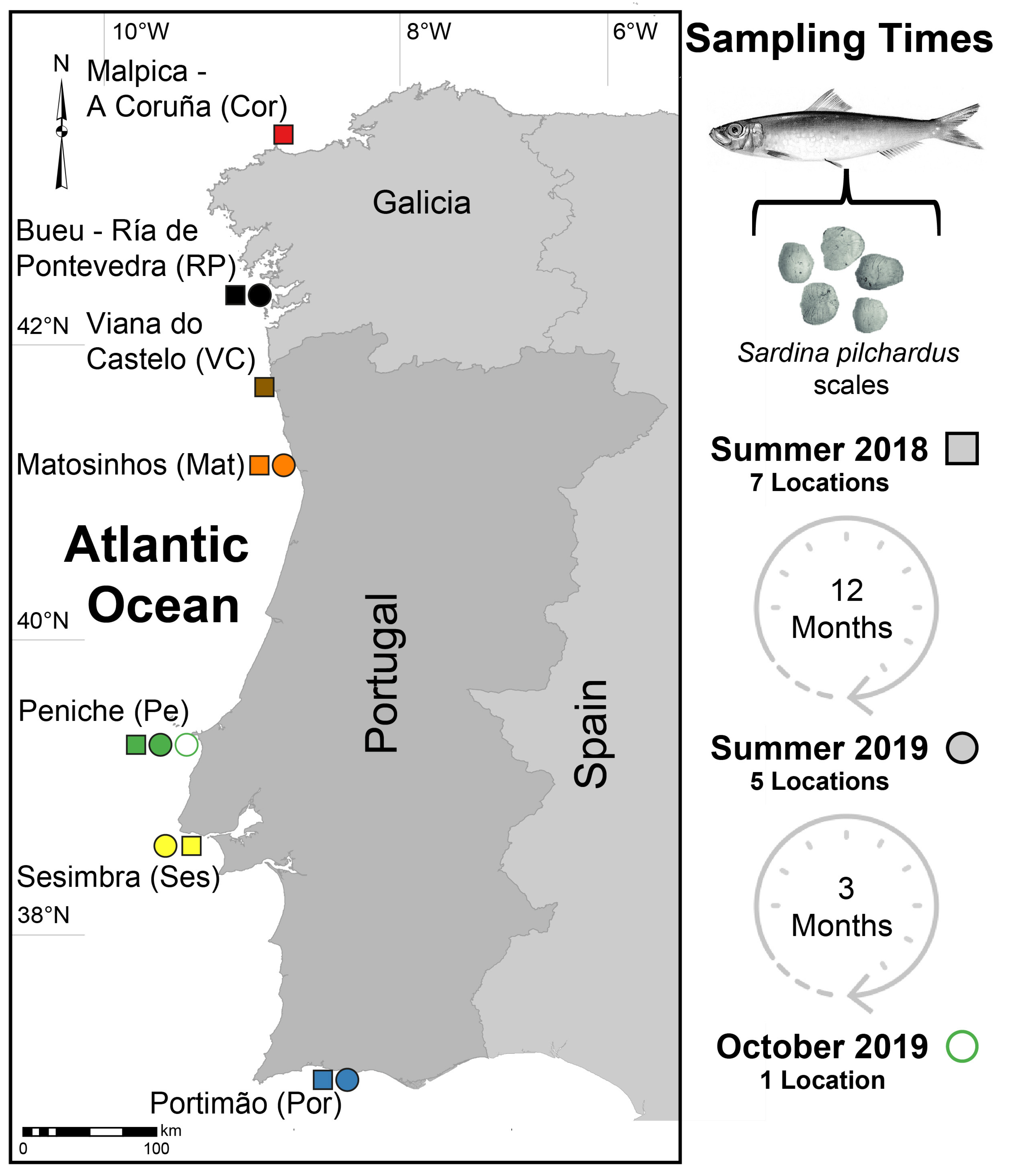
Figure 1. Sampling locations and sampling times of European sardines Sardina pilchardus along the Atlantic NW, W, and SW Iberian coasts. Squares (□) represent samples collected in 2018; and circles (○) represent samples collected in 2019. Color scheme: Cor—Red; RP—Black; VC—Brown; Mat—Orange; Pe—Green; Pe-Oct—White with green border; Ses—Yellow; Por—Blue. Malpica—A Coruña (Cor, 43°19′25.1″ N 8°48′29.3″ W), Bueu—Ría de Pontevedra (RP, 42°19′39.0″ N 8°47′06.9″ W), Viana do Castelo (VC, 41°41′09.1″ N 8°50′14.0″ W), Matosinhos (Mat, 41°10′59.8″ N 8°41′52.2″ W), Peniche (Pe, 39°21′20.6″ N 9°22′19.8″ W), Sesimbra (Ses, 38°26′24.7″ N 9°06′45.7″ W), and Portimão (Por, 37°07′58.6″ N 8°31′33.6″ W).
Fishes 11 00138 g001
Figure 2. Elemental concentrations (mg·kg−1) in scales of European sardine Sardina pilchardus collected in 2018 from fishing harbors in Galicia (Spain) and mainland Portugal along the NW, W, and SW Iberian coasts. Malpica—A Coruña (Cor), Bueu—Ría de Pontevedra (RP), Viana do Castelo (VC), Matosinhos (Mat), Peniche (Pe), Sesimbra (Ses), and Portimão (Por). Different letters (a–f) indicate significant differences between locations. Color scheme: Cor—Red; RP—Black; VC—Brown; Mat—Orange; Pe—Green; Ses—Yellow; Por—Blue.
Fishes 11 00138 g002
Figure 3. Elemental concentrations (mg·kg−1) in scales of European sardine Sardina pilchardus collected in 2019 from fishing harbors in Galicia (Spain) and mainland Portugal along the NW, W, and SW Iberian coasts. Bueu—Ría de Pontevedra (RP), Matosinhos (Mat), Peniche (Pe), Peniche—October (Pe-Oct), Sesimbra (Ses), and Portimão (Por). Different letters (a–e) indicate significant differences between locations. Color scheme: RP—Black; Mat—Orange; Pe—Green; Pe-Oct—White with green border; Ses—Yellow; Por—Blue.
Fishes 11 00138 g003
Figure 4. (A) Boruta result plot and (B) multidimensional scaling (MDS) ordinations of proximity scores of the Random Forest classifier based on the elemental fingerprints of European sardine Sardina pilchardus scales collected in 2018 from fishing harbors in Galicia (Spain) and mainland Portugal along the NW, W, and SW Iberian coasts. Malpica—A Coruña (Cor), Bueu—Ría de Pontevedra (RP), Viana do Castelo (VC), Matosinhos (Mat), Peniche (Pe), Sesimbra (Ses), and Portimão (Por).
Fishes 11 00138 g004
Figure 5. (A) Boruta result plot and (B) multidimensional scaling (MDS) ordinations of proximity scores of the Random Forest classifier based on the elemental fingerprints of European sardine Sardina pilchardus scales collected in 2019 in fishing harbors in Galicia (Spain) and mainland Portugal along the NW, W, and SW Iberian coasts. Bueu—Ría de Pontevedra (RP), Matosinhos (Mat), Peniche (Pe), Peniche—October (Pe-Oct), Sesimbra (Ses), and Portimão (Por).
Fishes 11 00138 g005
Figure 6. (A) Boruta result plot and (B) multidimensional scaling (MDS) ordinations of proximity scores of the Random Forest classifier based on the elemental fingerprints of European sardine Sardina pilchardus scales collected in 2018 and 2019 from five fishing harbors along the Atlantic NW, SW, and W Iberian coasts. Bueu—Ría de Pontevedra 2018 (RP 2018), Bueu—Ría de Pontevedra 2019 (RP 2019), Matosinhos 2018 (Mat 2018), Matosinhos 2019 (Mat 2019), Peniche 2018 (Pe 2018), Peniche 2019 (Pe 2019), Sesimbra 2018 (Ses 2018), Sesimbra 2019 (Ses 2019), Portimão 2018 (Por 2018), and Portimão 2019 (Por 2019).
Fishes 11 00138 g006
Table 1. Confusion matrices of the Random Forest classifications based on the elemental fingerprints of European sardine Sardina pilchardus scales collected from fishing harbors in Galicia (Spain) and mainland Portugal along the NW, W, and SW Iberian coasts. Malpica—A Coruña (Cor), Bueu—Ría de Pontevedra (RP), Viana do Castelo (VC), Matosinhos (Mat), Peniche (Pe), Peniche—October (Pe-Oct), Sesimbra (Ses), and Portimão (Por).
Predicted LocationTotal per Group% Correct
(Out-of-Bag All Samples)
ModelOriginCorRPVCMatPeSesPor
Model 2018Cor280020003093.3
RP129000003096.7
VC002720103090.0
Mat0003000030100
Pe001029003096.7
Ses000102903096.7
Por000100293096.7
Average classification success 95.7
RPMatPePe-OctSesPor
Model 2019RP28001013093.3
Mat02901003096.7
Pe02280003093.3
Pe-Oct000300030100
Ses000030030100
Por120002730100
Average classification success 95.6
Table 2. Confusion matrix of geographic origin predictions of European sardine Sardina pilchardus collected in 2019 using the reference model developed with samples from 2018 collected in fishing harbors in Galicia (Spain) and mainland Portugal along the NW, W, and SW Iberian coasts. Malpica—A Coruña (Cor), Bueu—Ría de Pontevedra (RP), Viana do Castelo (VC), Matosinhos (Mat), Peniche (Pe), Peniche—October (Pe-Oct), Sesimbra (Ses), and Portimão (Por).
Predicted LocationTotal per Location% Correct (Location)
CorRPVCMatPeSesPor
Based on the Reference Model 2018Original Location 2019
(12 months after the collection of specimens employed to assemble the predictive model)
RP00001290300
Mat00201270300
Pe000024603080.0
Pe-Oct0010020003066.6
Ses00270102300
Por00000300300
Average classification success 24.4
Table 3. Confusion matrix of the Random Forests classifications based on the elemental fingerprints of European sardine Sardina pilchardus scales collected in 2018 and 2019 from five fishing harbors along the Atlantic NW, W, and SW Iberian coasts. Bueu—Ría de Pontevedra 2018 (RP 2018), Bueu—Ría de Pontevedra 2019 (RP 2019), Matosinhos 2018 (Mat 2018), Matosinhos 2019 (Mat 2019), Peniche 2018 (Pe 2018), Peniche 2019 (Pe 2019), Sesimbra 2018 (Ses 2018), Sesimbra 2019 (Ses 2019), Portimão 2018 (Por 2018), and Portimão 2019 (Por 2019).
Origin
(Location × Year)
Predicted Origin (Location × Year)Total per
Location × Year
% Correct
(Out-of-Bag All Samples)
RP 2018RP
2019
Mat 2018Mat
2019
Pe 2018Pe 2019Ses 2018Ses 2019Por 2018Por 2019
RP 2018290000010003096.7
RP 2019028000100013093.3
Mat 20180030000000030100
Mat 2019000280011003093.3
Pe 20180000300000030100
Pe 2019000012810003093.3
Ses 2018011000280003093.3
Ses 20190000000300030100
Por 2018001000002903096.7
Por 2019020200000263086.7
Average classification success 95.3
Disclaimer/Publisher’s Note: The statements, opinions and data contained in all publications are solely those of the individual author(s) and contributor(s) and not of MDPI and/or the editor(s). MDPI and/or the editor(s) disclaim responsibility for any injury to people or property resulting from any ideas, methods, instructions or products referred to in the content.