1. Introduction
Fish are a rich source of high-quality protein, essential amino acids, and other nutrients often lacking in plant-based diets. They are crucial for maintaining a healthy, balanced diet for humans, and fish farming has consistently expanded over nearly three decades. In fish farming, fish counting plays a pivotal role in enhancing overall aquaculture productivity by enabling farm managers to formulate well-informed feeding plans, evaluate hatchery efficiency, monitor growth progress, and set suitable selling prices [
1,
2]. Currently, fish counting in aquaculture mainly relies on labor-intensive manual methods. However, these outdated practices are inefficient and prone to subjective errors, often causing physical harm and stress to the fish [
3,
4].
With the continuous advancement of machine vision technology, its advantages in terms of efficiency, speed, and cost-effectiveness have become increasingly significant. As a result, there is a growing trend in research to adopt machine vision methods for the precise fish counting. Based on the counting approach, it can be categorized into static counting and dynamic counting. Static counting involves enumerating fish within individual images, whereas dynamic counting processes video streams, necessitating the application of object tracking algorithms to continuously track and count fish within the counting area. Static counting is notably fast and efficient for small batches of fish but necessitates batch-wise counting. For large-scale counting, it is necessary to divide the fish into multiple batches, with each batch having a density that cannot be too high, which significantly affects counting efficiency. Moreover, the process of batch separation itself imposes a certain degree of stress on the fish. Dynamic counting enables the enumeration of fish as they continuously pass through the counting zone, eliminating the need for batching or pauses, thereby enhancing overall efficiency.
In the process of two kinds of fish counting, the fundamental task is to perform rapid and accurate detection of fish in images. Initial methods for fish detection primarily employed digital image processing techniques such as connected component analysis [
5,
6], blob detection [
7], or skeletonization [
8] to directly identify fish within an image. Alternatively, combining feature extraction and classifier for recognizing and regressing fish quantities in the Region of Interest (ROI) [
9,
10,
11]. However, these conventional methods are highly sensitive to environmental conditions and struggle to accurately detect and localize adherent or occluded fish. This is particularly evident in high-density aquaculture, where the slender and flexible morphology of fish frequently results in severe mutual overlapping and boundary ambiguity, creating a detection bottleneck that makes precise localization extremely difficult for standard algorithms.
In recent years, deep learning (DL)-based detection approaches have emerged as the leading solution, encompassing both density estimation-based and object detection-based methodologies [
12]. The density estimation-based methods utilize the convolutional neural network (CNN) model to extract fish features and subsequently generate a density map, from which the total number of fish in a single image is derived through integration [
1,
13,
14]. Object detection-based methods utilize target detection models to regress bounding boxes and central coordinates, enabling the precise localization of individual fish. There are two primary categories of target detection models: one-stage models and two-stage models. One-stage models, such as YOLO (You Only Look Once) and SSD (Single Shot MultiBox Detector), directly predict bounding boxes and class probabilities in a single pass through the network, which makes them generally faster. In contrast, two-stage models like Fast R-CNN (Region-based Convolutional Neural Network), Faster R-CNN, and Mask R-CNN [
15,
16,
17] involve region proposal and refinement stages, offering higher accuracy at the cost of increased computational demands compared to one-stage models [
18]. In the realm of object detection algorithms, the YOLO framework stands out due to its remarkable balance between speed and accuracy, enabling it to swiftly and reliably identify objects within images [
19]. The integration of parameter-efficient, high-accuracy lightweight network models into edge devices or smartphones for real-time fish detection has garnered increasing attention [
20].
One-stage object detection models have emerged as the preferred approach in related research. However, current one-stage efforts in fish detection mainly focus on incremental improvements to existing lightweight models and are typically tested on public datasets or in open-water environments. While detection in open waters primarily targets abundance estimation under variable conditions, industrial aquaculture demands high-precision quantification for breeding, sales, and stocking. Consequently, utilizing controlled environments—such as flow channels or conveyor belts—has become a standard engineering practice and a prerequisite for automated counting systems [
21]. By employing fixed channels with supplementary lighting, uncontrollable factors like turbidity and variable light are effectively mitigated. Under these standardized engineering conditions, the research focus rightfully shifts from environmental adaptation to the most critical remaining bottleneck: achieving robust and accurate individual identification amidst the physical complexities of high-density aquatic streams.
High-density fish counting in controlled environments faces specific and severe challenges [
22,
23]. Unlike open waters, high-density aquaculture ponds often suffer from complex lighting conditions caused by water surface reflections and artificial illumination.
More importantly, unlike general objects which possess rigid structures and distinct features, fish are non-rigid bodies characterized by slender, flexible morphologies. Their continuous deformation and highly similar textures lead to severe occlusion and ambiguous boundaries among individuals [
24], making standard feature extraction methods less effective in differentiating instances within dense clusters. While the standard YOLO series has achieved remarkable success in general object detection, it exhibits specific weaknesses in this scenario. The original architecture often struggles to extract fine-grained features from small, densely packed objects, leading to frequent missed detections in highly overlapped areas. Furthermore, standard loss functions are not sensitive enough to provide the precise localization required for accurate counting-oriented detection. Consequently, there remains a relative scarcity of literature that delves deeply into addressing these specific detection challenges arising from the slender body shape and severe overlapping of fish.
To bridge these gaps, the primary research objective of this study is to develop a lightweight yet high-precision fish detection model tailored for high-density aquaculture scenarios. The main contributions are as follows:
A lightweight fish detection network named YOLO-FC (YOLO constructed specifically for Fish Counting Applications) has been constructed based on the YOLO framework, with its parameter count and computational complexity being only 14.7% and 73.2%, respectively, of those in YOLOv5n (the nano version of YOLOv5) [
25].
A streamlined single-head detection structure was designed specifically for fish detection to enhance both precision and recall. Furthermore, Switchable Atrous Convolution (SAC) and Weighted Feature Fusion (WFF) were integrated into the network to improve model resilience against occlusion.
The model was optimized by adopting the EIOU loss and its modified Inner EIOU version, and the most effective scaling ratio (0.6) for auxiliary bounding boxes was determined. These adjustments improved the overall detection efficiency and precision.
The nano YOLO-FC was evaluated on a fish dataset, demonstrating precision, recall, and average precision metrics that outperform existing mainstream lightweight detection models and dedicated fish detection models.
The generalizability of the proposed model was validated by extending the evaluation to a shrimp larvae dataset. This assessment confirmed that the architecture maintains robust detection capabilities across different high-density aquatic species, effectively extending its applicability beyond the primary fish dataset.
2. Related Work
When it comes to fish counting based on DL-based detection technology, the environment in which the fish lives can be divided into an open environment and a controlled environment. Fish detection in open environments uses underwater or surface cameras to detect fish in open waters (such as marine environments or breeding ponds). The detection accuracy for underwater fish can be enhanced by fusing features extracted from multiple pathways [
26], such as the DP-FishNet [
27] and the Composited FishNet [
28]. However, these methods typically improve detection performance by increasing network complexity without explicitly accounting for real-time constraints in the detection process. YOLO-Fish [
29], DM-YOLO4 [
30], and CME-YOLOv5 [
31] are examples where researchers have improved upon existing YOLO models by incorporating various optimization techniques. These enhancements result in better performance, as evidenced by validation on their self-built datasets, showing a notable improvement over the baseline models. In open-water environments, accurate fish detection and counting are difficult due to uncontrollable factors, limited visibility, and clustering. Therefore, estimates are typically used instead of exact counts.
In controlled aquaculture settings, where accurate fish counting is critical for sales, breeding evaluations, and restocking activities, the process involves capturing images of fish in a controlled environment and then using detection models to identify and count them within designated areas precisely. Density estimation-based detection methods can be effectively employed for fish counting within single images [
1,
13,
14]. But these methods cannot get the specific location information about individual fish, and they can only yield the total number of fish in a single image, which cannot be applied to dynamic counting [
6].
The use of multi-object tracking methods, which combine detection techniques (including image processing [
6,
7], one-stage object detection models [
3], to multi-task learning [
32]) with tracking capabilities, enables real-time and continuous counting of fish within the counting channel. This approach is referred to as dynamic counting, where fish are counted in motion over time rather than in isolated snapshots. In controlled environments, the image background tends to be cleaner, whereas high-throughput counting scenarios frequently entail densely packed schools of fish within the counting area, along with severe occlusions. And the rapid movement of the fish results in deformation and motion blur, posing significant challenges for accurate detection. Moreover, given the wide variety of fish species in aquaculture, fish detection algorithms must also adapt to different breeds and sizes, which adds a layer of complexity to the already challenging task of fish detection.
Detection serves as the fundamental premise for counting, wherein the precision of fish detection directly influences the accuracy of the count. Meanwhile, the speed of detection is a pivotal determinant of the counting throughput. Factors primarily affecting detection velocity include the computational load and the number of parameters in the detection model. Consequently, to achieve high-throughput fish counting under controlled conditions, it is imperative and significant to develop a lightweight yet highly accurate fish detection model that mitigates these computational constraints.
3. Methodology
The YOLO model is a real-time object detection model, primarily composed of three major components: the Backbone, Neck, and Head. The Backbone network serves as the core component of the YOLO model. Through a series of convolutional layers and down-sampling operations, it derives feature maps at different scales, which encapsulate rich information about the input image. The Neck network, positioned between the Backbone and Head, is primarily designed for multi-scale feature fusion. This fusion enhances the model’s performance when dealing with objects of various sizes. In YOLOv3 [
33] and later versions, techniques like Feature Pyramid Network (FPN) and Path Aggregation Network (PAN) [
34] are introduced, which effectively aggregate features from multiple levels to provide a rich feature pyramid for the Head to utilize.
The Head network constitutes the output section of the YOLO model, responsible for generating the final prediction results, including the locations of bounding boxes and their class probabilities. The Bounding Box Regression (BBR) loss function is a critical component of the localization branch within detectors, and the accuracy of the detector’s localization heavily relies on bounding box regression. Consequently, the BBR loss function plays an indispensable role in contemporary detection frameworks. The following primarily introduces several components, loss functions, and the overall framework applied within the YOLO architecture in this study.
3.1. Switchable Atrous Convolution
Switchable Atrous Convolution (SAC) is an advanced convolutional mechanism designed to enhance feature extraction in object detection and segmentation tasks.
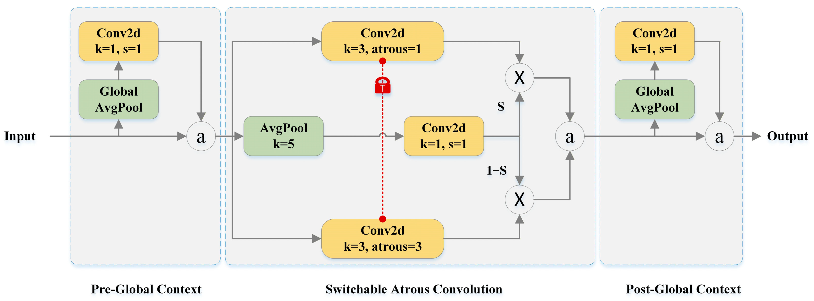
Figure 1 illustrates the specific implementation of SAC, which apart from the SAC component itself, comprises two global context modules. The SAC can express a conventional convolution as follows:
The notation represents a convolution operation where is the input, is the output, and denotes the set of weights, with representing the dilation rate.
In SAC, there is a 5 × 5 kernel and a 1 × 1 average pooling layer preceding the switch function. The switch function is a 1 × 1 convolutional layer that allows for independent control at each position, thus rendering the output more adaptable and versatile. And two additional branches utilize convolutions with different dilation rates to enhance the performance of the object detector when dealing with objects of various sizes and potentially accelerate the training process. Moreover, SAC incorporates two lightweight global context modules placed before and after the main component. Through these innovative designs and mechanisms, SAC enhances the adaptability of the network when processing features across different scales and complexities while maintaining lower model complexity and computational resource consumption, which is particularly beneficial for capturing the long-range dependencies of slender fish bodies that standard convolutions might miss.
3.2. Weighted Feature Fusion
PAN introduces global self-attention upsampling to restore pixel localization, with conventional methods typically treating all input features equally. However, given that different input features at varying resolutions usually contribute unequally to the output representation, Tan et al. [
36] devised an approach where each input is assigned an additional learnable weight to allow the network to discern the importance of each input feature. This is achieved through a Weighted Feature Fusion (WFF) mechanism. The model combines these features by performing a weighted sum or aggregation based on their associated weights, generating a fused feature vector. This process enables the model to dynamically adjust the contributions of each type of feature according to its significance, thereby allowing it to capture information from diverse patterns and potentially overcome the limitations of single modalities. Moreover, by assigning specific weights to each feature layer, it emphasizes features more crucial for object detection, thereby enhancing the effectiveness and expressive power of the features and mitigating the feature ambiguity caused by transparent or low-contrast fish targets.
WFF involves multiple approaches, including Unbounded Fusion, Softmax-Based Fusion, and Fast Normalized Fusion. Unbounded fusion can achieve comparable accuracy to other methods with minimal computational cost, but the scalar weights being unbounded may lead to unstable training. Softmax-based fusion yields the best results, yet its application on GPU hardware often incurs significant performance degradation; Fast normalized fusion, however, delivers a similar level of precision as softmax-based fusion while being up to 30% faster [
36]. Consequently, the fast normalized fusion approach was ultimately adopted in this study. The Fast normalized fusion method is as follows:
, where
is non-negative,
denotes the input feature map at the
-th level; and
= 0.0001 is a small value introduced to avoid numerical instability.
3.3. Feature Extraction Components
GSConv (Group Shuffle Convolution) is a lightweight convolution technique tailored for object detection tasks that can reduce model complexity without compromising accuracy, thereby enhancing inference speed. Building upon GSConv, we integrate the bottleneck structure from YOLOv5 [
25], as depicted in
Figure 2a, to form the GSBottleNeck module shown in
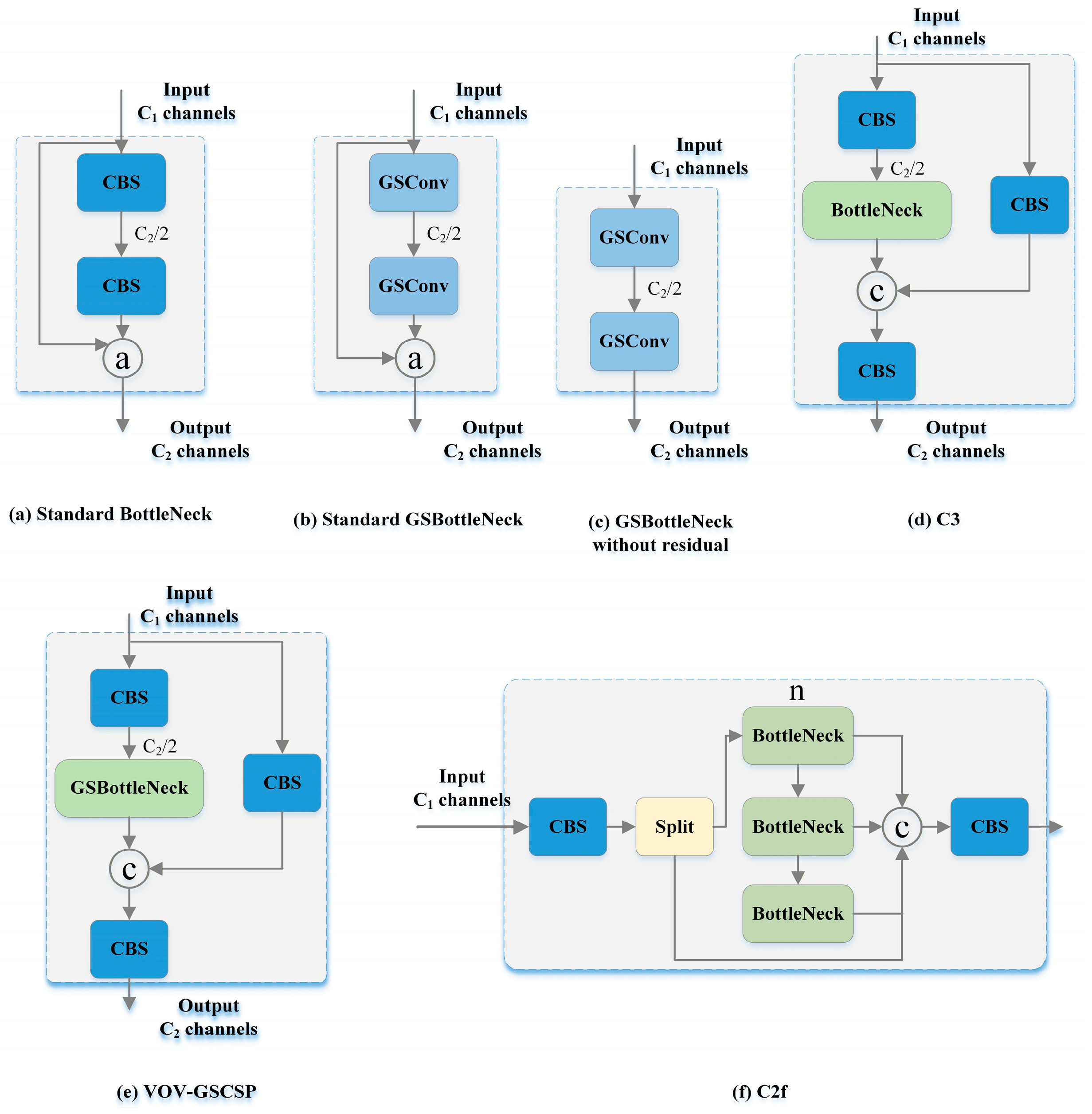
Figure 2b. In a standard bottleneck design, there exists a shortcut branch that effectively learns residual features and improves network depth. Additionally, there exists a structure known as the “bottleneck without residual” in bottleneck, which consists solely of two stacked standard convolutions or GSconvs, as illustrated in
Figure 2c.
As shown in
Figure 2d, the C3 module in YOLOv5 splits input channels, processes them independently with convolutional operations, then merges them to create a design that economizes computations while bolstering information flow. The VOVGSCSP module, akin to the C3 module in YOLOv5, replaces the standard bottleneck with a GSBottleNeck, as shown in
Figure 2e. This modification lowers computational complexity and network architecture intricacy while maintaining adequate accuracy. As depicted in
Figure 2f, the C2f module in YOLOv8 [
37] features more skip connections than the C3 module and incorporates additional split operations, removing convolutional operations in the branches. This design allows for retaining lightweight characteristics while gaining richer gradient flow information, strengthening feature representation, and reducing computational overhead.
3.4. Bounding Box Regression Loss Function
In the context of BBR, Intersection over Union (IOU) loss effectively quantifies the degree of overlap between predicted bounding boxes and ground truth (GT) boxes, thereby ensuring that the model learns to capture the positional information of targets during training accurately. Up to now, Intersection over Union (IOU)-based loss functions (
) have gradually become mainstream in the field. Most existing methods are built upon or extend the concept of IOU, such as GIOU [
38], DIOU [
39], SIOU [
40], and EIOU [
41].
While the existing BBR loss functions effectively boost convergence and detection capabilities by adding geometric constraints to IOU-based losses, they do not tackle the core rationality of the IOU-based loss itself, which significantly affects detection accuracy. To correct this flaw, Zhang et al. [
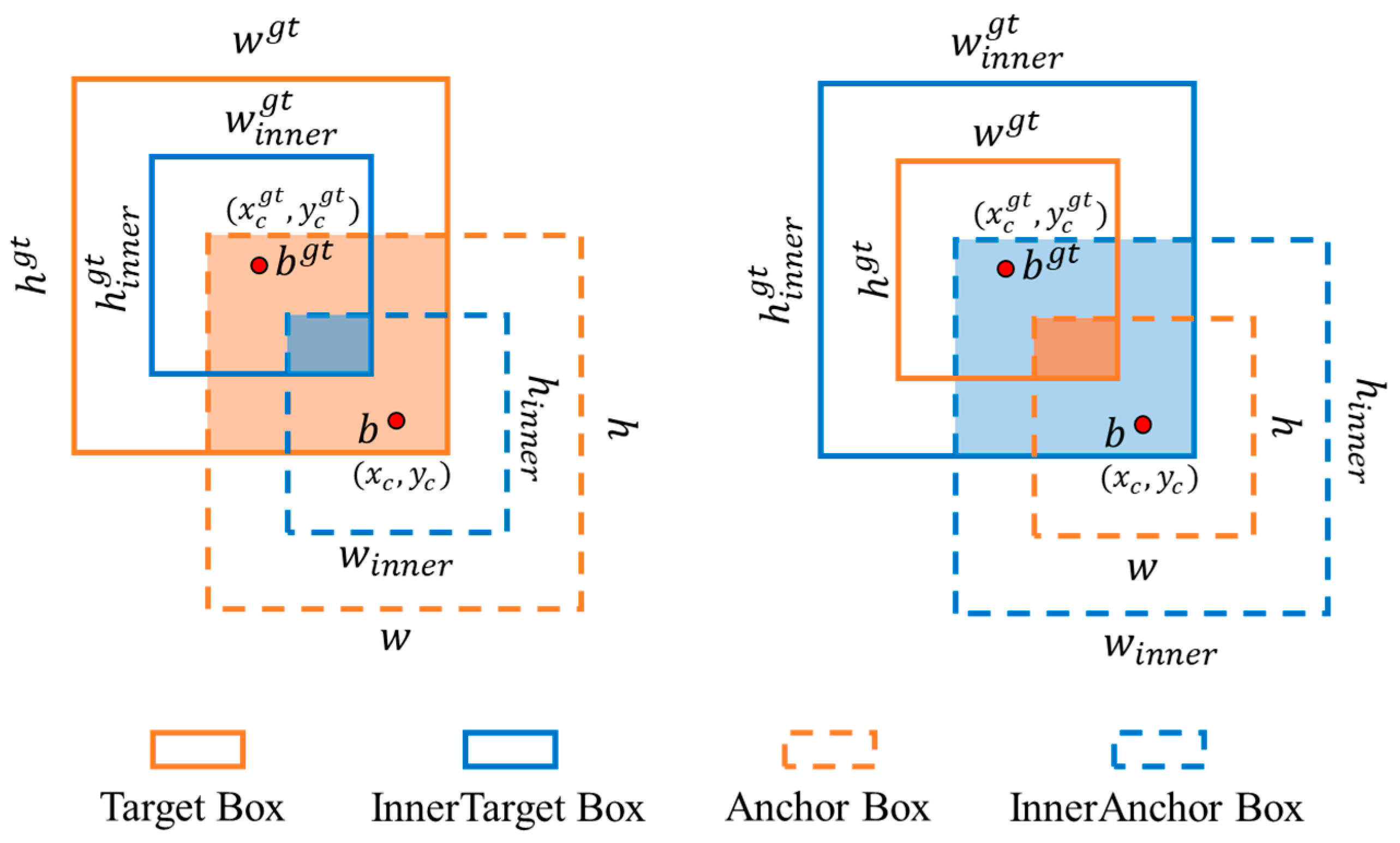
42] revisited the IOU loss function and introduced Inner-IoU, which uses auxiliary bounding boxes for regression to speed up convergence without requiring extra loss components. The Inner-IoU presents a scaling factor ratio to control the size of this auxiliary bounding box, as shown in
Figure 3. The Inner-IoU is defined as follows:
The GT bounding box and anchor box are denoted as and B, respectively. The center point of GT and the inner GT are represented by (, ), while the center point of the anchor box and inner anchor box are represented by (, ). The variable corresponds to the scaling factor.
In comparison to IOU, Inner-IoU has a narrower regression scope when
< 1 and the auxiliary box is smaller than the anchor box. It also generates larger gradient values, which speeds up convergence, particularly for high IOU samples, by enabling more precise adjustments towards the ground truth during training. Conversely, when
exceeds 1, a bigger auxiliary box widens the regression range using Inner-IoU, which helps enhance the regression performance for low IOU samples. Applying Inner-IoU to existing IOU-based BBR loss functions (like
) can be defined as follows:
3.5. Model Structure
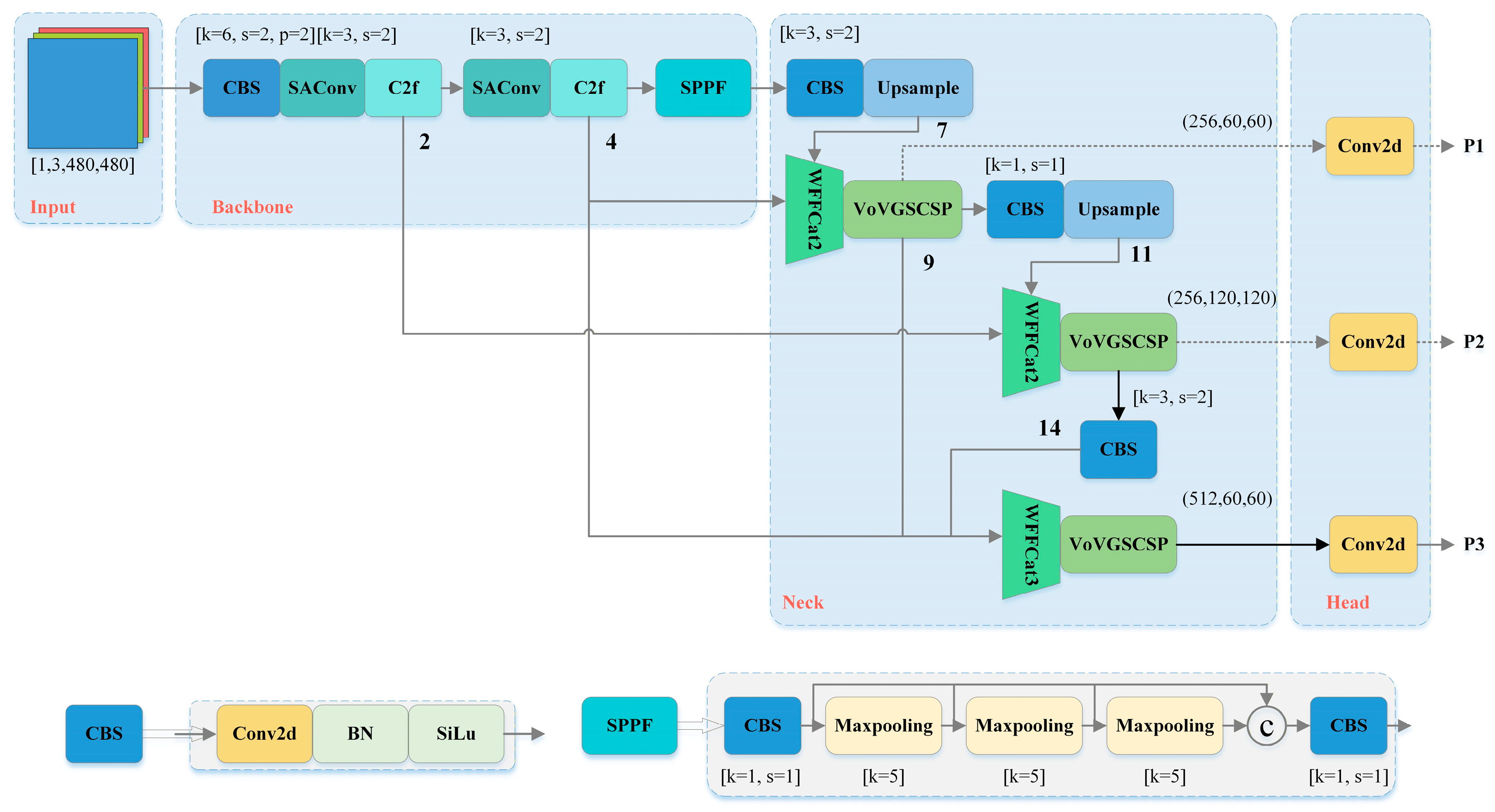
To accelerate the computation in prediction, images fed into a CNN must undergo a similar transformation process within the Backbone: spatial information is progressively transferred to the channel domain. Each time a feature map’s spatial dimensions (width and height) are compressed and its channels expanded, some semantic information is inevitably lost. To achieve efficient fish detection, a YOLO-FC model was constructed, as depicted in
Figure 4. In order to mitigate information loss while preserving the capacity to extract salient features, the backbone of the YOLO-FC model was judiciously equipped with one CBS module and two SAC and SPPF modules, and the C2f module was introduced to enhance the network’s feature extraction capabilities. The backbone network of YOLO-FC comprises merely six components, with meticulous adjustments made to the input and output dimensions of feature maps for each component.
Fusing features from different scales of feature layers effectively accommodates fish of varying sizes. In the neck network of YOLO-FC, upsampling operations, along with WFF and VOVGSCSP, are adopted for further feature fusion to provide higher-level semantic information and adaptability to images of different scales. The first fusion comes from feature layers {4, 7}; the second fusion originates from layers {2, 11}, and the third fusion combines feature maps from {4, 9, 14}. The three-fold fusion offers information from varying depths, encompassing abundant shallow feature information that can effectively capture more detailed information, thus benefiting the identification and localization of adhered fish. Notably, in the neck of YOLO-FC, there are only two instances of upsampling. In the head section, P2 generates the largest-sized feature map; P1 and P3 generate feature maps of the same size. In the feature map outputted by P3, features from P2 are fused. To reduce computational load, instead of further increasing the dimensions of the P3 output feature map, its spatial size is decreased while the number of channels is augmented.
3.6. Model Evaluation
In this study, the size of parameter count (Params) is utilized to represent the complexity of the network. At the same time, computational cost is expressed in terms of Floating-Point Operations per second (FLOPs). For object detection algorithms, precision (
), recall (
), and average precision (
) are commonly employed as performance metrics. The calculation methods are as follows:
The confusion matrix resulting from the evaluation procedure provides the following explanation of the testing outcomes: True Positives (), False Positives (), False Negatives (), and True Negatives (). The performance measure, Average Precision (), is defined as the area under the curve. A higher value signifies increased precision in predicting diverse object classes. Additionally, represents the calculated across an IOU range from 0.50 to 0.95 with increments of 0.05; while specifically denotes the when the IOU threshold is set at 0.5.
4. Results and Discussion
4.1. Fish Dataset
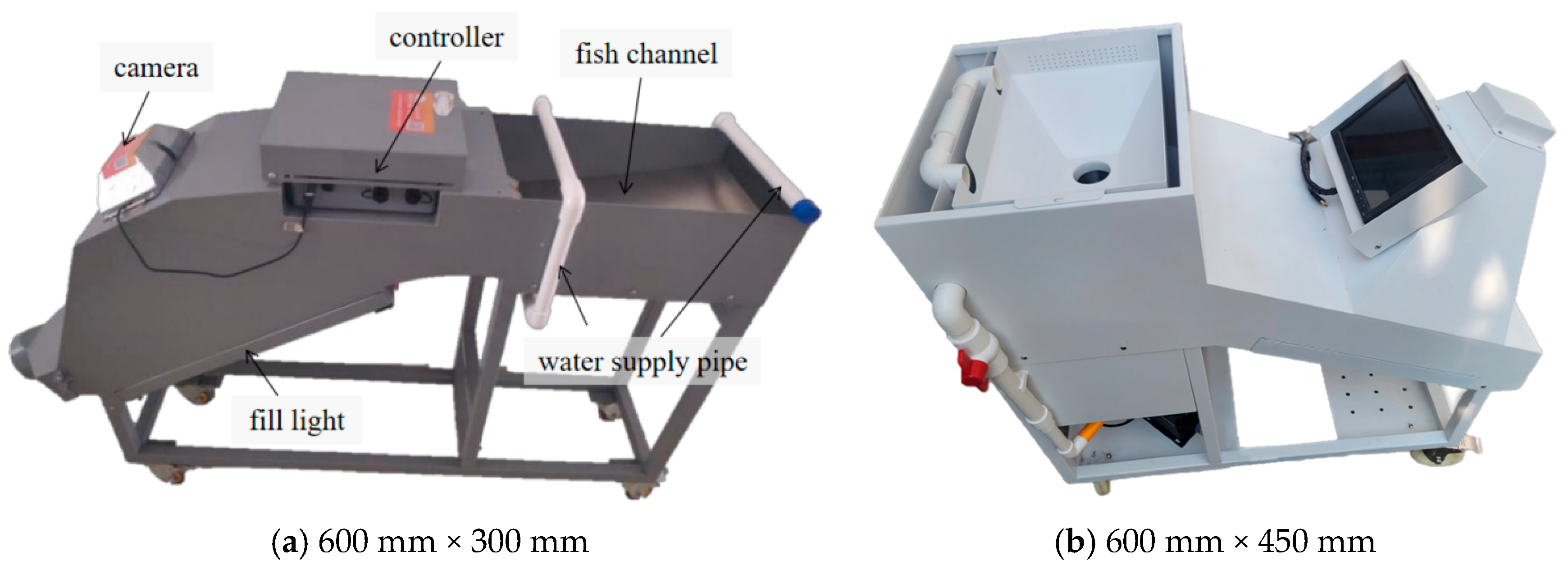
The datasets used in this study were collected using counters constructed based on the counting principle proposed by Zhou et al. [
6]. These counters consist of a fish channel, fill light, a camera, and a water supply system. The fill light is installed at the bottom of the fish channel to provide adequate illumination for the enclosed channel.
Figure 5 illustrates the two experimental prototypes with different channel dimensions used for data collection in this study. As fish flow through the channel with the water current, a camera positioned at the top of the channel captures real-time data on the passing fish. Currently, such counters are being manufactured by Hainan iAQUA Technology Co., Ltd., Haikou, China.
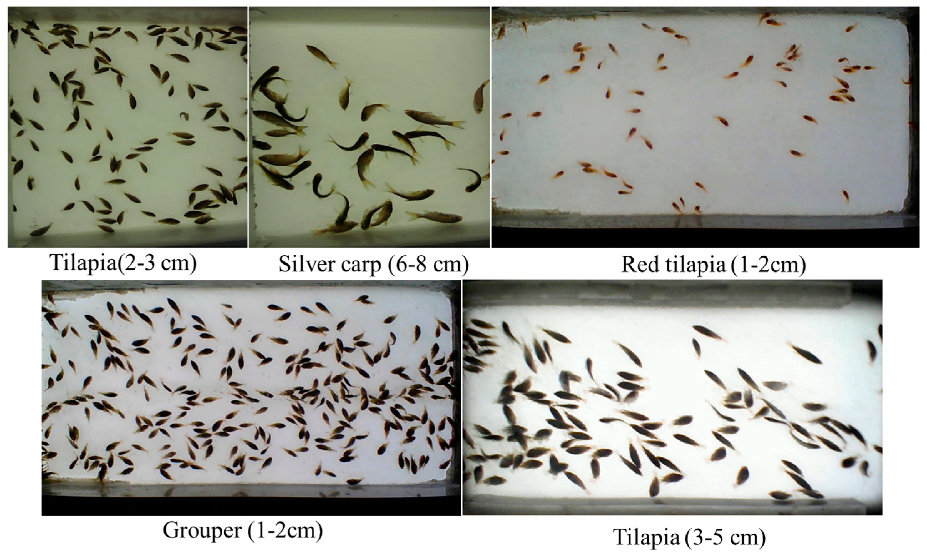
The dataset consists of images collected by different versions of counters, as shown in
Figure 6, featuring backgrounds under three distinct lighting conditions and encompassing five species and sizes: tilapia (
Oreochromis mossambicus, in size ranges of 1–2 cm, 2–3 cm, and 3–5 cm), grouper (
Epinephelus, 1–2 cm), and silver carp (
Hypophthalmichthys molitrix, 6–8 cm). The dataset has been filtered to exclude images containing only a few fish, ensuring that the distribution of fish within each image is relatively dense. The variations in background of the collection device, fish sizes, species, and distribution densities illustrate the diversity of the dataset utilized in this study. In total, there are 2845 images in the dataset, which have been randomly divided into training and validation sets at an 8:2 ratio. To ensure a fair and unbiased comparison, all models involved in this study—including the proposed YOLO-FC and other different detection models—were trained and evaluated using the exact same dataset partition (8:2 split).
The annotations for this dataset were carried out using LabelImg, and YOLO format text annotation files were generated accordingly. It can be observed in
Figure 6 that the distribution of fish within the channel is indeed quite dense, with numerous instances of adhesion between them. Due to the similarity in features and identical colors, it can sometimes even be challenging for humans to distinguish individual fish within these adhered regions. Moreover, larger-sized fish often exhibit deformation and motion blur. Additionally, aside from dark borders present around some of the images, fish located near the edges of the channels may produce reflections along those edges, adding complexity to the scene. All these intricate circumstances pose certain challenges to achieving high accuracy in detecting fish.
4.2. Experimental Configuration
In this study, the hardware configuration for testing the model includes an Intel Core i5-13400F CPU (Intel Corp., Santa Clara, CA, USA) operating at 2.5 GHz and a GeForce RTX 3080 GPU (NVIDIA Corp., Santa Clara, CA, USA). The software setup consists of the Windows 10 operating system (Microsoft Corp., Redmond, WA, USA), the PyTorch (1.13.1) DL framework (Meta Platforms, Inc., Menlo Park, CA, USA), and the Python (3.8) programming language (Python Software Foundation, Wilmington, DE, USA). During training, the initial learning rate was set to 0.01, the number of epochs was configured as 100, and the batch size was set to 16.
Furthermore, in the course of training, data augmentation was appropriately applied with a certain probability to account for conditions encountered during fish counting. This augmentation included enhancements to the three-channel space of HSV of images, as well as image rotation and cropping, among other techniques. Experimental setup parameters are listed in
Table 1, while all other parameters were kept consistent with those of YOLOv5 [
25] version 7.0.
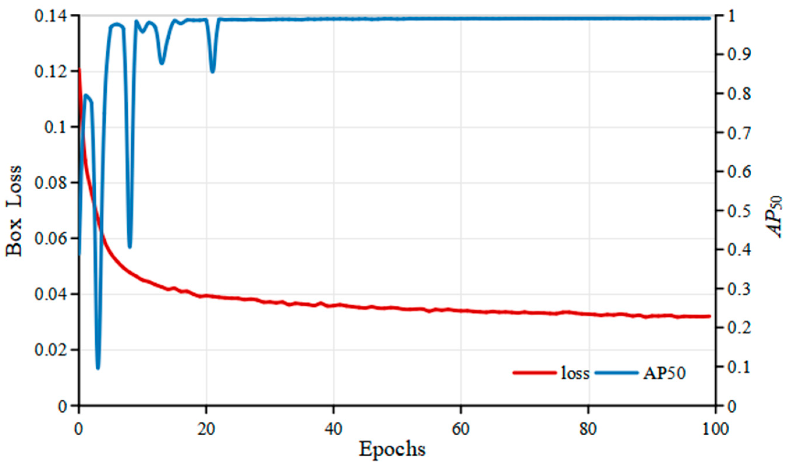
To verify the training stability and convergence speed of the proposed model under these configurations, the training process was visualized. As presented in
Figure 7, the box loss curve demonstrates a rapid decline during the initial 50 epochs and stabilizes thereafter, indicating effective feature learning. Meanwhile,
rises steadily and plateaus around the 80th epoch, confirming that the model converges well without exhibiting signs of overfitting.
4.3. Optimization of Network Performance
4.3.1. The Number of Detection Heads
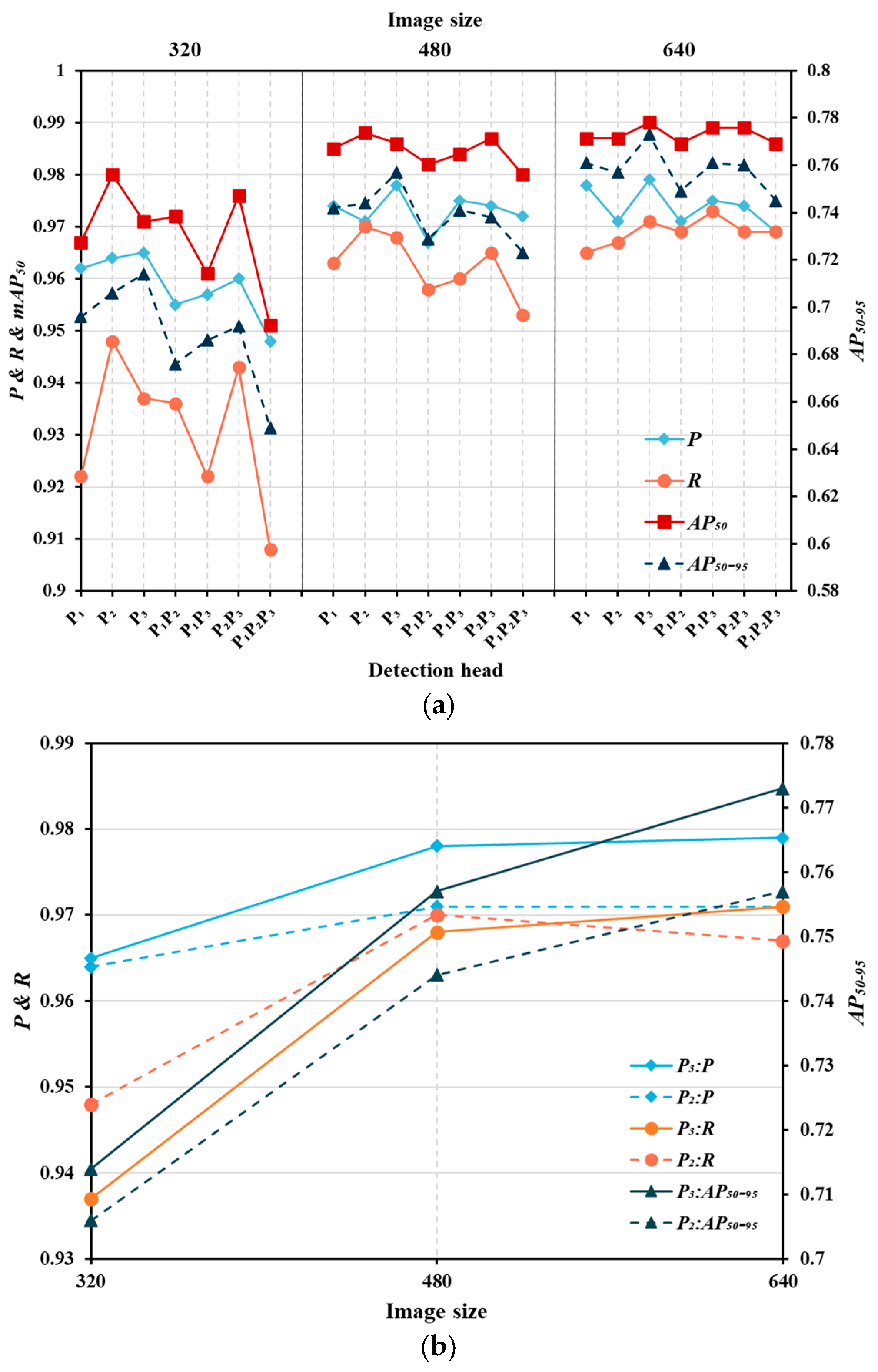
In order to enhance detection accuracy and efficiency, YOLO has undergone continuous iteration and updates, incorporating various improvement strategies. In YOLO versions after v3, a design extracts object details at multiple scales using three distinct feature maps with individual detection heads. This method strengthens small object detection while maintaining performance for larger objects. However, it increases computational demands and model size due to the multi-scale detection heads. In practical applications such as fish detection where the distance between the camera and the fish remains fixed and the size variation (1–10 cm) among the counted fish is relatively small—meaning there are no large targets but primarily small to medium-sized ones—the need for multiple scale detection might be less critical. Moreover, given the relatively simple and uniform characteristics of fish, an excessive number of detection heads might lead to information redundancy that could potentially hinder detection performance. To validate this hypothesis, we conducted experiments by combining different detection heads and testing them on three distinct detection maps with resolutions of 3 × 320 × 320, 3 × 480 × 480, and 3 × 640 × 640. The results of these tests are illustrated in
Figure 8, providing insight into the optimal configuration for our specific application scenario.
From
Figure 8a, it can be observed that there are significant differences in detection performance when using various combinations of detection heads. When solely utilizing the P3 detection head, it exhibits the best overall detection performance (
) across all three image sizes. When employing two detection heads for detection tasks, despite maintaining a constant computational load and parameter count, the overall detection performance (
) on each of the three differently sized detection maps shows a decline compared to using the P3 head alone, with a decrease ranging from 1.2% to 3.8%. In contrast, adopting a combination of three detection heads (P1P2P3) results in the poorest overall detection performance (
) across all three image sizes. This substantiates that, for fish with simple features and similar scales, employing multiple detection heads can lead to a decrease in detection performance.
Comparing the use of single detection heads (P1, P2, and P3) individually, P1 consistently exhibits the poorest detection performance across all three image sizes. A possible reason for this is that the neck feature fusion network in P1 is relatively shallow, which might not fully extract and integrate the fish features. In contrast, the P2 detection head corresponds to a larger-sized feature map, while the P3 detection head benefits from a deeper network structure. As
Figure 8b shows, when the detection image size is 3 × 320 × 320, the P2 detection head exhibits a notable advantage in recall rate (+1.1%) compared to the P3 detection head; however, the P3 detection head’s
improves by 0.7% relative to that of P2. As the size of the detection images increases, the advantages of the P3 detection head over the P2 detection head become more pronounced across all four metrics. This suggests that the P2 detection head, which utilizes larger-sized feature maps, is beneficial for detecting objects within smaller-scale images. In contrast, the P3 detection head, with its deeper feature map outputs, possesses superior localization performance and scale adaptability. Consequently, this study bases its subsequent optimization efforts on the model employing only the P3 detection head as the foundational model.
4.3.2. Loss Function and Parameter Optimization
In order to further select the optimal loss function, we also conducted tests on different loss functions using images of size 3 × 480 × 480 for detection. The results are presented in
Table 2. From
Table 2, it can be observed that when employing SIOU, the detection performance achieves the best
p-value at 97.9%. On the other hand, when using EIOU, both
and
metrics yield the best results, showing an approximate improvement of about 0.2% compared to SIOU. Considering these outcomes comprehensively, the EIOU was chosen to build the loss function.
Additionally, incorporating the concept of Inner-IoU (Intersection over Union), the bounding boxes are scaled according to a scaling ratio
, which generates auxiliary regression boxes. In order to identify the optimal scaling ratio, a series of tests were conducted on different values of
. The results of these tests are presented in
Table 3. From
Table 3, it can be discerned that when
> 1, the performance in terms of
and
are equivalent to their values at
= 1 (standard IOU); however,
and
respectively decrease by 0.3% and 0.2% compared to their values at
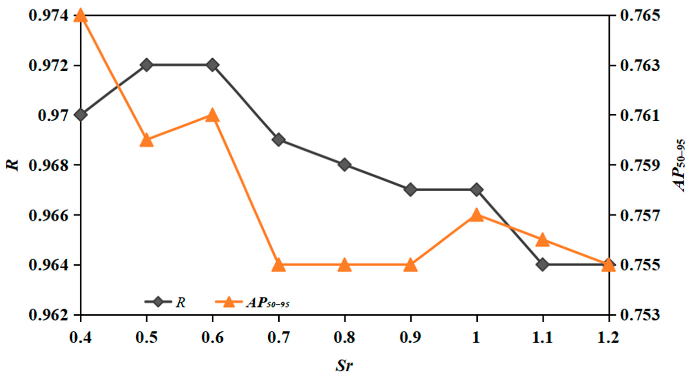
= 1. This suggests that, in the context of the fish detection task in this study, the fish data samples are predominantly high IOU samples. As shown in
Figure 9, reducing the value of
effectively improves detection performance. When the value of
is in the range [0.7–1],
and
do not exhibit significant changes, with the primary influence being on R and
. When
= 0.6, both
,
,
and
show a considerable improvement compared to
, with increases of 0.1%, 0.5%, 0.2% and 0.4%, respectively. However, as
continues to decrease to 0.5 and 0.4,
and
experience a decline, indicating that an overly small
can negatively affect the BBR. Therefore, for the specific detection task under consideration in this study, the optimal range for
is between 0.5 and 0.7. Consequently, for our subsequent optimization experiments, we choose
to be 0.6.
4.3.3. Ablation Experiments
Within the context of the ablation experiments, we examined the impact of different modules on the performance of fish detection, including the SAC within the backbone network, the WFF, the VOVGSCSP module and the C3 module within the neck network. As seen in
Table 4, upon replacing the C3 module with the VOVGSCSP module within the neck network, there is a significant decrease in both the number of parameters and computational load. This change predominantly influences the measure
, resulting in a drop between 0.5% and 1.3%. The influence on the remaining three metrics, on the other hand, is less than 0.2%. Replacing standard convolutions in the backbone network with SAC can efficiently decrease the model’s computational load. However, this comes with a corresponding increase in the model’s parameter count and inference time. In contrast, using WFF for feature fusion does not significantly affect either the model’s inference time or its parameter size.
When SAC and WFF are employed separately, there could be a marginal variation of about 0.2% in different detection indicators. When the neck network utilizes the VOVGSCSP module, configurations incorporating SAC, WFF, and the VOVGSCSP module without shortcut branches achieve optimal scores across all three metrics: P, , and , with a near-optimal R of 97.2%. In contrast, when the neck network employs the C3 module, setups with SAC, WFF, and the C3 module featuring shortcut connections reach their peak in at 77.2%, while maintaining sub-optimal performance in the other three indicators. These outcomes demonstrate that the combined employment of SAC and WFF contributes to ensuring the model’s robustness effectively.
Furthermore, the inference times for individual models on a single image span between 5.3 ms and 6.5 ms, and we regard a difference of roughly 1 ms as being within a tolerable range, essentially meeting the demands of practical applications. However, pursuing substantial performance enhancements could entail bearing higher computational costs.
4.4. Comparative Experiments
4.4.1. Compare with Mainstream Models
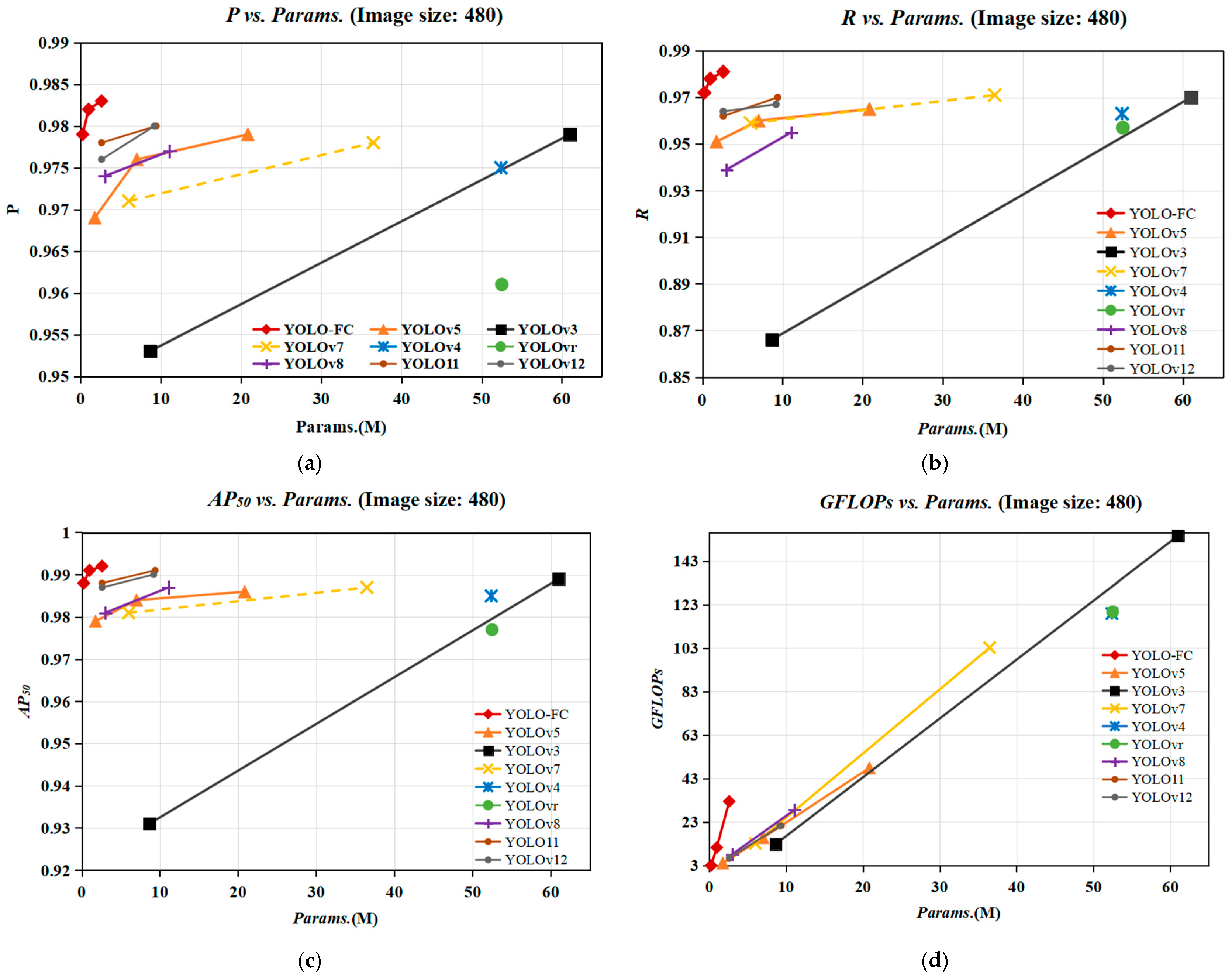
The proposed YOLO-FC model was compared with mainstream YOLO models, and the results are illustrated in
Figure 10 and
Table 5. It can be observed that across all models, as the parameters increase, there is a noticeable improvement in various performance metrics. Among the existing models, YOLOv3 [
33], YOLOR [
43] and YOLOv4 [
44] all have relatively large parameter counts and computational load. As shown in
Figure 10, when comparing models with similar parameter amounts, YOLOv5 [
25], YOLOv7 [
45], YOLOv8 [
37], YOLO11 [
46], YOLOv12 [
47] demonstrate significantly higher detection performance than their predecessors, such as YOLOv3, YOLOR, and earlier versions. Specifically, YOLOv7-tiny exhibits an impressive boost of 9.3% in R over YOLOv3-tiny, showcasing its enhanced efficiency and effectiveness for object detection tasks.
In comparing the nano and small model of YOLOv8 with their respective counterparts in YOLOv5, the differences in and metrics are less than 0.5%. However, YOLOv8 models show an improvement of 4.5% to 4.9% in compared to YOLOv5 models. Despite this, the for YOLOv8 is lower by 0.5% to 1.2% when contrasted with YOLOv5. The main cause of the lower in YOLOv8 is due to its use of an anchor-free approach, which might not be as effective as anchor-based methods in accurately localizing and bounding densely packed objects, leading to a decreased .
Compared to other models, YOLO-FC features smaller parameters and lower computational requirements. When the parameter count is similar, YOLO-FC demonstrates comprehensive improvements across all metrics. For instance, when comparing the nano, small and medium models of YOLO-FC and variants with their respective counterparts in YOLOv5, there are enhancements in all four indicators, especially in
and
. In terms of
, YOLO-FC shows increases of 2.1%, 1.8%, and 1.6% respectively. Meanwhile in
, it surpasses by 4.1%, 3.6%, and 3.2%. Meanwhile, YOLO-FC also outperforms several improved versions of YOLOv5 (such as TP-YOLO [
48], TPH-YOLOv5 [
49]) in terms of all evaluation metrics. When compared against the nano and small models of YOLOv8, while YOLO-FC has slightly lower
scores by 0.9%, and it significantly surpasses the performance in metric R, showing a consistent improvement of 3.3% for two models. Additionally, YOLO-FC exhibits a 0.5–0.7% advantage over the nano and small models of YOLOv8 in both
and
. Comparisons with YOLO11 and YOLOv12 indicate that increasing model complexity yields limited performance gains in this specific task. Although these models achieve slightly higher
, they have approximately 8.7 times the parameters of YOLO-FCn yet exhibit lower Recall rates compared to the 97.2% achieved by YOLO-FCn. This suggests that the complex feature extraction structures of general-purpose models may introduce redundancy when detecting uniform fish targets. These models tend to focus on rich texture details rather than the boundary information essential for separating adhered individuals. In contrast, YOLO-FC demonstrates that a simplified architecture can achieve competitive accuracy and effectively reduce missed detections with significantly lower computational costs. The comparison results demonstrate the superior performance of YOLO-FC in the fish detection tasks.
4.4.2. Comparing the Models with Different Size
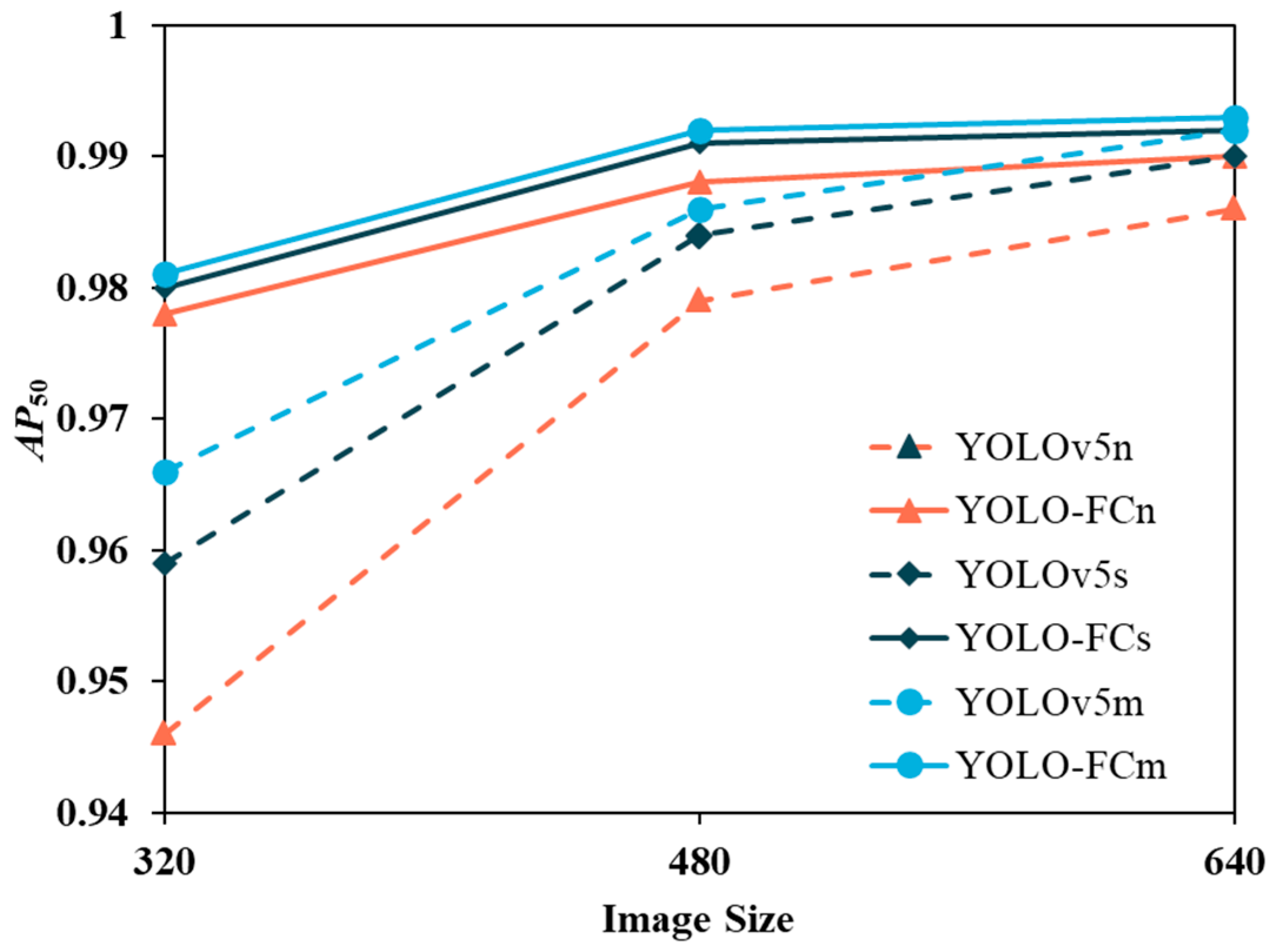
Figure 11 presents a comparison of the test results for YOLO-FC and three differently scaled models of YOLOv5 [
25], each operating on image sizes of 320, 480, and 640 pixels. The parameter count and computational load of YOLO-FC are only 14.7% and 73.2% of those in YOLOv5, respectively. However,
Figure 11 demonstrates that YOLO-FC exhibits significant improvements over YOLOv5, with the nano of YOLO-FC variant even surpassing the medium of YOLOv5 in terms of
. Additionally, it can be observed across all models that
generally increases as the image size grows; however, the rate at which
rises tends to taper off with larger image dimensions. This suggests that once the model architecture is fixed, there is a limit to how much detection performance can improve solely by increasing image resolution—beyond a certain point, enhancing the image size does not lead to further gains in detection capability. These data aid us in understanding how to optimize model performance by adjusting image size and also shed light on the differences between various approaches.
It is worth noting that with the increase in model size, the impact on detection performance continually decreases. Although YOLO-FCm has over twice the number of parameters compared to YOLO-FCs, the boost it provides in terms of , , and is minimal, just 0.2%. Furthermore, the influence of model size on detection performance in YOLO-FC seems to be significantly lower than that of YOLOv5, which is mainly due to the commendable detection performance offered by the network framework introduced in this study.
4.4.3. Compare with Other Fish Detection Models
Furthermore, the comparative experiments between YOLO-FC and existing fish detection models (YOLO-Fish [
29], DM-YOLO4 [
30], and CME-YOLOv5 [
31]) were also conducted, where training and evaluation were performed on a custom-built dataset, as shown in
Table 6. It is evident that currently, the CME-YOLOv5 model outperforms both the remaining two existing models, achieving an impressive 98.2% in
. The YOLO-fish model is an improvement based on YOLOv3 [
33], while DM-YOLOv5 represents an enhancement to YOLOv5 [
25]; despite substantial reductions in both parameter count and computational complexity compared to their respective base models, their performance on the dataset is less favorable, particularly for DM-YOLOv5, which records an
score of only 91.5%. Although CME-YOLOv5 exhibits a modest improvement over YOLOv5 across four metrics, ranging from 0.2% to 0.4% increase within the context of our dataset evaluation, YOLO-FC demonstrates even better performance. In direct comparison, YOLO-FC surpasses CME-YOLOv5 in
by 1.2%,
by 1.7%,
by 0.6%, and
by 5.3%. This comprehensive set of results clearly highlights the superiority of YOLO-FC in real-time fish detection under controlled environment.
4.4.4. Generalizability Analysis on Shrimp
To verify the broad applicability of the proposed model, a shrimp larvae dataset was introduced for further validation. This dataset comprises 3172 images captured using mobile phones in actual production environments, divided into a training set of 2537 images and a validation set of 635 images. Compared to fish, shrimp larvae are characterized by their minute size, high transparency, and a strong tendency to cluster in extremely high densities, posing a significantly greater detection challenge.
Experimental results in
Table 7 indicate that YOLO-FCn has only 0.3 M parameters, representing approximately 1/10th of YOLOv8n [
37] and 1/6th of YOLOv5n [
25]. Despite this small model size, it achieves a Recall of 96.0%, outperforming all comparative models. This signifies an effective reduction in missed detections, which is critical for accurate counting in aquaculture. Furthermore, its Precision (97.0%) and
(98.0%) remain on par with the larger YOLOv8n and YOLOv12n [
47] models.
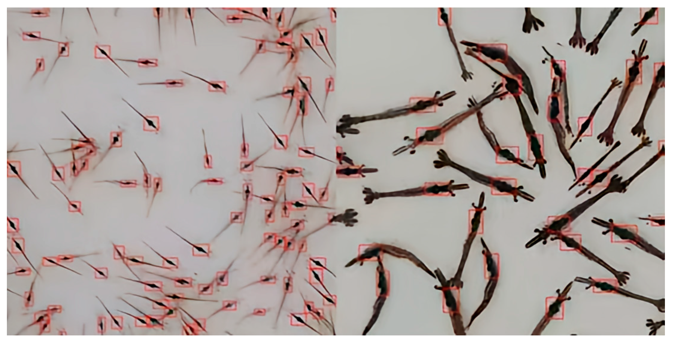
Figure 12 illustrates the qualitative detection results. These findings confirm that the model not only outperforms comparative models on the original fish dataset but also exhibits no performance degradation when transferred to the distinct shrimp dataset. This demonstrates that the proposed lightweight strategies are not overfitted to specific fish features but possess strong robustness, maintaining superior detection performance across diverse aquatic species.
4.5. Discussion
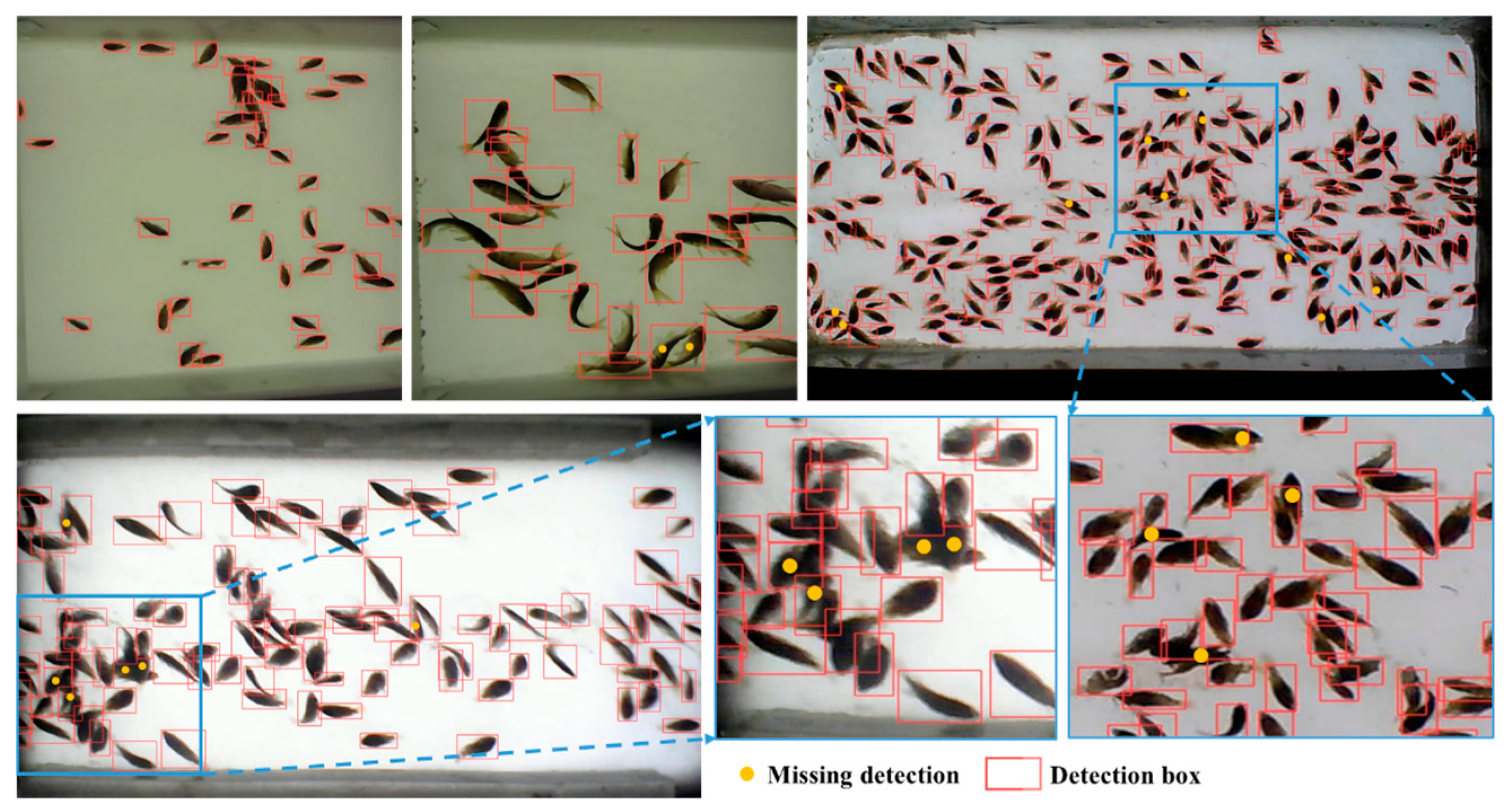
Figure 13 presents a series of actual detection outputs from the model, clearly demonstrating that YOLO-FC maintains a relatively high level of detection accuracy and robustness even under conditions with densely distributed fish populations. This strong generalizability is further corroborated by the evaluation on the shrimp larvae dataset (
Table 7), where the model achieved a superior Recall of 96.0%, confirming that the integrated SAC and WFF modules effectively mitigate feature ambiguity across diverse aquatic species.
The superior performance of YOLO-FC stems from architectural adaptations explicitly tailored to the biological characteristics of fish and the specific constraints of the counting environment. By streamlining the network to a single detection head, the model eliminates the redundancy of multi-scale detection for uniformly sized targets, effectively reducing false positives caused by background noise. To capture the features of non-rigid, slender fish bodies that constantly deform during swimming, the SAC module introduces an adaptive receptive field that dynamically adjusts to varying body curvatures, thereby improving recall. Furthermore, the WFF mechanism mitigates severe occlusion in high-density streams by prioritizing distinct edge features over ambiguous signals in overlapping areas. These targeted optimizations allow YOLO-FC to achieve high precision while maintaining lightweight efficiency.
However, an analysis of typical failure cases reveals certain limitations when dealing with situations where fish are adhered or piled up to a significant extent. As shown in the magnified area within
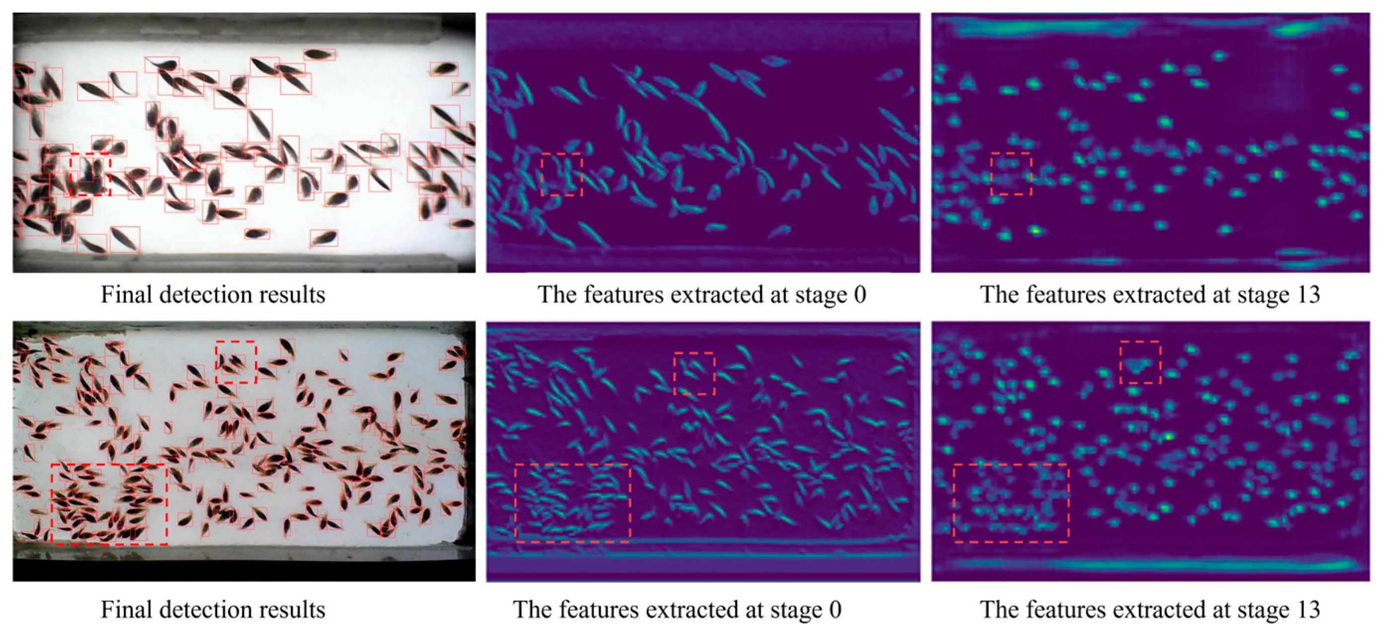
Figure 13, when fish are densely stacked to a certain degree, even manual differentiation becomes challenging in accurately distinguishing individual fish, leading to missed detections in terms of identification and localization by the model. Upon further examination of the intermediate detection feature maps (as seen in
Figure 14), it can be observed that under dense stacking conditions, the model’s extraction of edge features becomes indistinct (especially in the region highlighted by a bounding box in
Figure 14), which could be a major contributing factor to the occurrence of missed detections. Moreover, due to increased spatial overlap between fish, the IOU between predicted bounding boxes grows larger. This may result in the NMS process inadvertently removing some genuinely valid detection results while eliminating redundant bounding boxes, thereby affecting the final detection precision.
Consequently, future research directions can focus on improving the YOLO-FC model’s capability to extract edge features, enhancing its resolution performance in scenarios involving adherent fish. Simultaneously, exploring more refined post-processing strategies, such as refining the non-maximum suppression algorithm to better adapt to high-density target scenes, would help reduce the likelihood of mistakenly discarding valid detection frames due to improperly set IOU thresholds. These series of optimization measures are expected to significantly boost the model’s target detection performance in various complex environments with clustered fish populations




 ,
,