Article

The Biogeographic Patterns of Two Typical Mesopelagic Fishes in the Cosmonaut Sea Through a Combination of Environmental DNA and a Trawl Survey

1
Deep Sea and Polar Fisheries Research Center, Key Laboratory of Mariculture, Ministry of Education, Ocean University of China, Qingdao 266100, China
2
School of Fishery, Zhejiang Ocean University, Zhoushan 316002, China
3
Polar Research Institute of China, Shanghai 200136, China
*
Author to whom correspondence should be addressed.
Fishes 2025, 10(7), 354; https://doi.org/10.3390/fishes10070354
Submission received: 9 June 2025 / Revised: 11 July 2025 / Accepted: 16 July 2025 / Published: 17 July 2025
(This article belongs to the Section Biology and Ecology)

Abstract

Investigating biodiversity in remote and harsh environments, particularly in the Southern Ocean, remains costly and challenging through traditional sampling methods such as trawling. Environmental DNA (eDNA) sampling, which refers to sampling genetic material shed by organisms from environmental samples (e.g., water), provides a more cost-effective and sustainable alternative to traditional sampling approaches. To study the biogeographic patterns of two typical mesopelagic fishes, Antarctic lanternfish (Electrona antarctica) and Antarctic deep-sea smelt (Bathylagus antarcticus), in the Cosmonaut Sea in the Indian Ocean sector of the Southern Ocean, we conducted both eDNA and trawling sampling at a total of 86 stations in the Cosmonaut Sea during two cruises in 2021–2022. Two sets of species-specific primers and probes were developed for a quantitative eDNA analysis of two fish species. Both the eDNA and trawl results indicated that the two fish species are widely distributed in the Cosmonaut Sea, with no significant difference in eDNA concentration, biomass, or abundance between stations. Spatially, E. antarctica tended to be distributed in shallow waters, while B. antarcticus tended to be distributed in deep waters. Vertically, E. antarctica was more abundant above 500 m, while B. antarcticus had a wider range of habitat depths. The distribution patterns of both species were affected by nutrients, with E. antarctica additionally affected by chlorophyll, indicating that their distribution is primarily influenced by food resources. Our study provides broader insight into the biogeographic patterns of the two mesopelagic fishes in the remote Cosmonaut Sea, demonstrates the potential of combining eDNA with traditional methods to study biodiversity and ecosystem dynamics in the Southern Ocean and even at high latitudes, and contributes to future ecosystem research and biodiversity conservation in the region.
Key Contribution: This study provides insights into the distribution of two mesopelagic fish species in the Cosmonaut Sea and reveals the significant influence of food resources on the distribution of these two fish species, contributing to future ecosystem studies and biodiversity conservation in the region. This is also the first time that environmental DNA (qPCR) has been applied to the study of mesopelagic fish distribution in the Southern Ocean.

1. Introduction

Mesopelagic fish, as a group of fishes inhabiting the upper 1000 m in the ocean, play an important role in the marine food web, connecting primary consumers such as zooplankton with advanced consumers such as birds, large fish, and marine mammals [1,2,3]. They are widely distributed across oceans worldwide, contributing significantly to the global fish biomass [4]. In the Southern Ocean, mesopelagic fishes, including bathylagids, myctophids, liparids, and zoarcids, are a major component of the fishes [5]. Antarctic lanternfish (Electrona antarctica), as a dominant species in the family of Myctophidae, is an endemic mesopelagic fish in the Southern Ocean [6]. It is distributed around Antarctica, occupying 200 to 1000 m of water from the Antarctic Polar Front to the high Antarctic latitudes [7,8]. Its distribution is mainly influenced by sea surface temperature [9,10,11] and krill abundance [12], while the distribution of juvenile fish is closer to the edge of sea ice [13]. The Antarctic lanternfish is not only abundant in resources, but it also has high energy and is rich in lipids, which is of great significance to the energy transfer independent of krill in the Southern Ocean [14,15,16]. Antarctic deep-sea smelt (Bathylagus antarcticus), which belongs to Bathylagidae, is also a dominant and endemic mesopelagic fish distributed around the Southern Ocean [17]. The catches of B. antarcticus have been among the top catches in previous Southern Ocean midwater trawl surveys, especially dominating at water depths of 400–1000 m [14]. Fishes of this family, especially the Antarctic deep-sea smelt, as the prey of species in higher trophic levels like toothfish, play a connecting role in the energy flow in the Antarctic food web [18]. It has been shown that Antarctic deep-sea smelt play the most dominant role in upward food web energy transfer in the southwest Pacific sector [19]. Given their ecological importance, accessing their resources and distribution is of great significance for the survival of top predators in Antarctica, as well as for understanding marine ecosystems and biogeochemical cycles [20,21].
At present, the biodiversity of Antarctic fish is primarily investigated using methods such as trawling, underwater vision, and acoustic technologies [22,23,24]. Conventional surveys may provide important information on fish species and populations; however, they are species-selective, destructive to biodiversity and habits, dependent on taxonomic knowledge [25,26], and challenged by logistical collection costs and the difficulty of reaching remote environments, particularly in the remote and extreme regions of Antarctica [27]. Effective and comprehensive methods for fish surveys are required for the better monitoring of aquatic organisms.
The environmental DNA (eDNA) approach, which has been increasingly popular in the detection of marine life in various aquatic ecosystems, including the Southern Ocean, may be a promising choice [26,27,28,29]. Environmental DNA refers to genetic materials collected from environmental samples (e.g., water, sediment, soil) that is shed by organisms [30]. Compared with traditional methods, this approach can detect species in the environment even at low biomass, offering finer species resolution and greater cost-effectiveness, with survey efficiency, costs, and the results being superior [27,31,32,33]. There are two primary methods for eDNA analysis: metabarcoding and qPCR (species-specific detection). The eDNA metabarcoding method detects the assemblage or community of a specific taxon (such as fish) in the environment by amplifying short fragments containing sufficient sequence variations to correctly identify species [34,35]. It can capture species information in the environment more widely and comprehensively. However, when focusing on a single or few species, the species-specific detection method tends to be more time- and cost-effective [36]. Quantitative PCR (qPCR) uses species-specific primers to amplify and detect short DNA fragments of target species [31]. Compared to metabarcoding, this method offers high sensitivity, specificity, and potential for quantifying target DNA and provides a better reflection of species biomass [37]. Therefore, the qPCR approach is typically used to evaluate the distribution of key species or invasive species [33,38,39].
The Cosmonaut Sea, located in the Indian Ocean sector of the Southern Ocean, serves as an important habitat for Antarctic lanternfish and Antarctic deep-sea smelt [40]. However, it remains one of the less studied regions of Antarctic waters. Historically, there were few scientific surveys of mesopelagic fishes that have been reported in the Cosmonaut Sea, resulting in a limited understanding of the diversity of fish species. The most recent trawl survey was conducted during the 36th Chinese Antarctic Research Expedition in 2020 [24], while other surveys were reported before 2010, where more attention was paid to the community structure of mesopelagic fishes based on trawl surveys, rather than the distribution pattern of a single target fish species [9,10,41,42]. Although there has been a recent eDNA metabarcoding study in this region [28], the study was more specific to fish biodiversity patterns in the pelagic waters, and the descriptions of single species are still not sufficiently detailed. Compared with other areas in the Southern Ocean, the Cosmonaut Sea has received less attention in revealing the species composition and ecosystem, and there is a lack of targeted studies on key mesopelagic species.
Based on the data from two cruises of the Chinese Antarctic Scientific Expedition (CHINARE) in 2021–2022, this study comprehensively used eDNA and trawl survey approaches to explore the following: (1) The spatial distribution patterns of Antarctic lanternfish (E. antarctica) and Antarctic deep-sea smelt (B. antarcticus) in the Cosmonaut Sea. (2) The effects of environmental factors on the distribution of two fish species. In addition, we also developed species-specific primers and probe sets for each of the two fish species, which can be applied to detect the eDNA of target fish in the environment. Our study aims to explore the spatial distribution of two typical mesopelagic fishes in the Cosmonaut Sea and their influencing factors while verifying the potential of eDNA for monitoring mesopelagic fishes in the Southern Ocean, providing the essential basic information and technical support for further studies on the oceanic ecosystem of the Cosmonaut Sea.

2. Materials and Methods

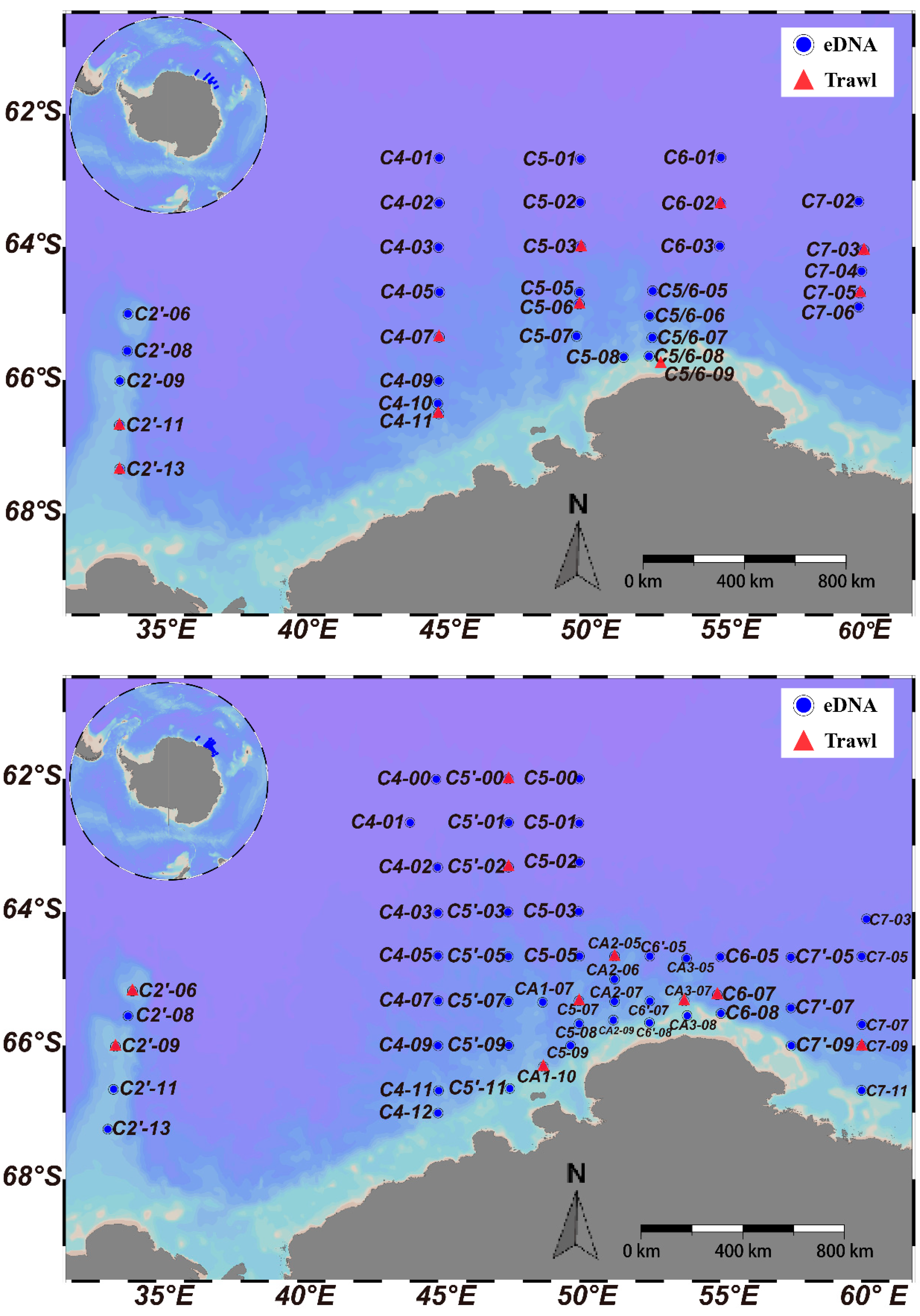
2.1. eDNA and Fish Sample Collection

The Cosmonaut Sea is located between 30°E and 60°E in the Indian Ocean sector of the Southern Ocean (Figure 1), extending to the eastern boundary of the Weddell Gyre in the west and bordering the Prydz Bay Gyre in the east [9,43]. Seawater samples were collected from the Cosmonaut Sea in the Southern Ocean from 5 to 26 January 2021 and 27 January to 11 March 2022, carried out with the polar icebreaker R/V Xuelong 2. A total of 187 eDNA samples were collected from 85 stations during the two cruises, including 62 samples collected from 32 stations in 2021 and 125 samples collected from 53 stations in 2022 (Figure 1 and Supplementary Table S1). At each station, approximately 1.5–5.0 L of water was collected at different water depths using Niskin bottles with an SBE 911 Plus CTD system (Sea-Bird Scientific, Bellevue, WA, USA). Water samples were immediately filtered onto a polycarbonate membrane (47 mm diameter with a pore size of 0.22 µm, Isopore, Merck-Millipore Inc., Darmstadt, Germany). Filter funnels were soaked in 10% sodium hypochlorite solution for at least one hour after use and washed with ultrapure water before the next filtration. New gloves were used for each sample. DNA tissue preservation buffer (Tiandz Inc., Beijing, China) was added to the filters and stored at −80 °C. Due to operational time and logistical difficulties in the Southern Ocean, no negative controls were collected.
Trawl surveys were conducted at 9 stations from 5 to 26 January 2021 and at 11 stations from 28 January to 7 March 2022 (Figure 1 and Supplementary Table S2). Mesopelagic fish samples were captured using a rectangular midwater trawl (RMT) with a 5 m2 effective mouth and consistent 1 cm mesh size cod-ends. Trawler speeds ranged from 2 knots to 3 knots, and the maximum sampling depth could reach 1458 m. The duration of each trawl was approximately 2 h. The captured fish were initially identified and frozen on board and then transported to a laboratory for further species identification and biological measurements. The weight of each specimen was measured with an electronic balance accurate to 0.1 g.
Environmental variables, including the total depth, sampling depth, longitude, latitude, temperature, salinity, dissolved oxygen concentration, colored dissolved organic matter (CDOM), and chlorophyll concentration of each seawater sample, were measured using CTD system technology; nutrients (NH4+, NO3, NO2, PO43−, SiO32−) were measured by the Polar Research Institute of China. Environmental variables were collected simultaneously with seawater. Distances from the station to land were extracted from the Global Marine Environment Datasets (GMED, http://gmed.auckland.ac.nz/ accessed on 24 January 2025).

2.2. Development of Specific Primers and Probes and qPCR Assays

Trawl-caught specimens were identified according to the lowest possible taxon level by morphology and DNA barcoding. DNA extraction and COI amplification were performed as in a previous study [44]. Specifically, genomic DNA was extracted using the TIANamp Marine Animals DNA Kit (Tiangen Biotech (Beijing) Co., Ltd, Beijing, China). The COI fragment was amplified using F1: TCAACCAACCACAAAGACATTGGCAC and R1: TAGACTTCTGGGTGGCCAAAGAATCA [45]. The total volume of the reaction was 25 μL and comprised 12.5 μL of PCR Mix (Beijing Tsingke Biotech Co., Ltd., Beijing, China), 9.5 μL of ddH2O, 1 μL each of forward and reverse primers (10 μmol/L), and 1 μL of genomic DNA. The reaction conditions were as follows: predenaturation at 94 °C for 5 min, followed by denaturation at 94 °C for 45 s, annealing at 55 °C for 45 s, extended at 72 °C for 45 s, 35 cycles, and extended at 72 °C for 10 min. The COI PCR products were sequenced by Shanghai Personal Biotechnology Co., Ltd., Shanghai, China, and verified using the NCBI sequence blast tool.
Species-specific primers and Taqman probes were designed in the COI region of the mitochondrial DNA using Beacon Designer 8.0 software. The mitochondrial COI sequences of Myctophidae and Bathylagidae were downloaded from NCBI and compared to design the specific primers and probe, while the COIs of E. antarctica and B. antarcticus were amplified using the specimens collected in the Cosmonaut Sea in 2021. Specificity was confirmed in silico and vitro. PrimerBlast on the NCBI website was used to verify primer specificity online. The experiments in vitro were conducted using mitochondrial genomic DNA from E. antarctica, B. antarcticus, and five other captured Antarctic fish species (Gymnoscopelus braueri, Krefftichthys anderssoni, Nannobrachium achirus, Cynomacrurus piriei, Lepidonotothen squamifrons) as templates for qPCR experiments.
The reaction mixture (20 μL) contained 10 μL of qPCR Mix (2 × AceQ Universal U+ Prob Master Mix V2, Vazyme Biotech Co., Ltd., Nanjing, China), 0.4 μL of each primer (10 μM, Beijing Tsingke Biotech Co., Ltd., Beijing, China), 0.2 μL of TaqMan Probe (10 μM, Beijing Tsingke Biotech Co., Ltd., Beijing, China), 4 μL of template DNA, and 5 μL of ddH2O. qPCRs were performed using an ABI StepOne Plus real-time PCR system (Thermo Fisher Scientific, Waltham, MA, USA). The reactions entailed activation at 37 °C for 2 min, denaturation at 95 °C for 5 min, and then 45 cycles of denaturation at 95 °C for 10 s and annealing and extension at 60 °C for 30 s. ddH2O was also used as a negative control to monitor pollution in the process of the PCR experiment. All samples were assayed in triplicate. The mean eDNA concentration was calculated for each sample as the mean of the three technical replicates.
The plasmids of the target fishes were used as standard samples for the qPCR assays. The target fragments of the two fish species were cloned into a plasmid vector (pUC57), followed by amplification and plasmid DNA extraction using a high-purity plasmid mini kit (Trelief Plasmid Mini Kit Plus, Tsingke, China). Plasmids were diluted to a series of standard samples that contained 100–109 copies of DNA molecules per 1 μL (Supplementary Tables S3 and S4). The standard curve for each qPCR assay was determined based on the Ct values and DNA copy numbers of standard samples. The quantity of eDNA was normalized against the volume of each filtered water sample.

2.3. Data Analysis

The fish biomass and abundance at each station were standardized as one hour of trawling. The copies obtained through qPCR were also standardized to 1 L of water production; then the copies were transformed by log10 (x + 1) to eliminate the effect of extreme and zero values. The sampling stations and spatial distribution of two fish species were visualized with Ocean Data View software (v5.6.3).
Considering the spatial differences in survey stations, we divided the stations into three categories based on water depth: shelf (0–1000 m), slope (1000–2000 m), and abyssal (>2000 m) stations (Supplementary Figure S1). There were 7, 16, and 62 sampling stations for each of the three types of stations. To explore the differences in the eDNA results sampled at different depths in the vertical direction, we defined five sampling layers based on the actual water depth, layer 1—surface; layer 2—10–200 m; layer 3—500 m; layer 4—1000 m; and layer 5—bottom (sampling depth = actual depth). There were 84, 7, 31, 39, and 26 samples in layers 1 to 5, respectively (Supplementary Table S1). Surface sampling was conducted at all stations (except C2′-06 in 2022), with the middle sampling layer (layer 2–4) of each station being determined based on the maximum water depth, and only one layer was sampled. The sampling of the middle and bottom layers was determined by on-site water allocation.
At each layer, we measured the eDNA detection rate, which is the number of samples with target species detected divided by the total number of samples collected. The eDNA sample was considered positive if at least one repeat of the eDNA sample amplified the target species. eDNA concentration was also measured as the amount of eDNA present in each volume of a sample (e.g., water,). eDNA presence/absence were defined as the detection/non-detection of the target species by qPCR, respectively.
Statistical differences in eDNA concentration by layers and stations were assessed using the Kruskal–Wallis test. Statistical differences in fish abundance and biomass between shelf, slope, and abyssal stations were assessed using the Mann–Whitney test. Box plots were generated using the “ggplot2” [46] package, and PCA diagrams were generated using the “FactoMineR” package [47] in R version 4.3.0 [48]. Mantel’s test and a Generalized Additive Model (GAM) were used to study the relationship between fish distribution and environmental factors. For eDNA, the environmental variable corresponded to the sampling depth of the sample, while for trawls, the environmental variables used the mean value from the surface to the maximum sampling depth. The model fitting was realized by the gam function of the “mgcv” package [49] in R, and the multicollinearity of the factor was judged by the VIF function of the “car” package [50]. Mantel’s test was performed using OmicStudio tools at https://www.omicstudio.cn/tool (accessed on 28 January 2025).

3. Results

3.1. Primer and Probe Design

A set of specific primers and probes was developed within the mitochondrial COI region for E. antarctica and B. antarcticus, respectively. For E. antarctica and B. antarcticus, the limit of detection (LOD), the limit of quantification (LOQ), and the amplicon length were 8 copies/4 μL and 12 copies/4 μL, 14 copies/4 μL and 18 copies/4 μL, and 107 bp (base pair) and 153bp, respectively (Table 1). The primers and probes were confirmed to be specific for the target fish both in silico and in vitro (Supplementary Figures S2 and S3). And no amplification signals were observed in PCRs using non-target species DNA as a template or negative controls (Supplementary Figure S4).

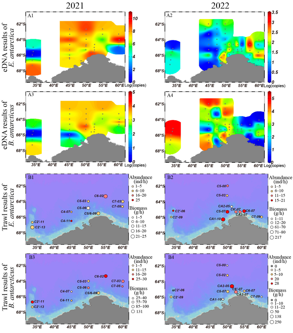
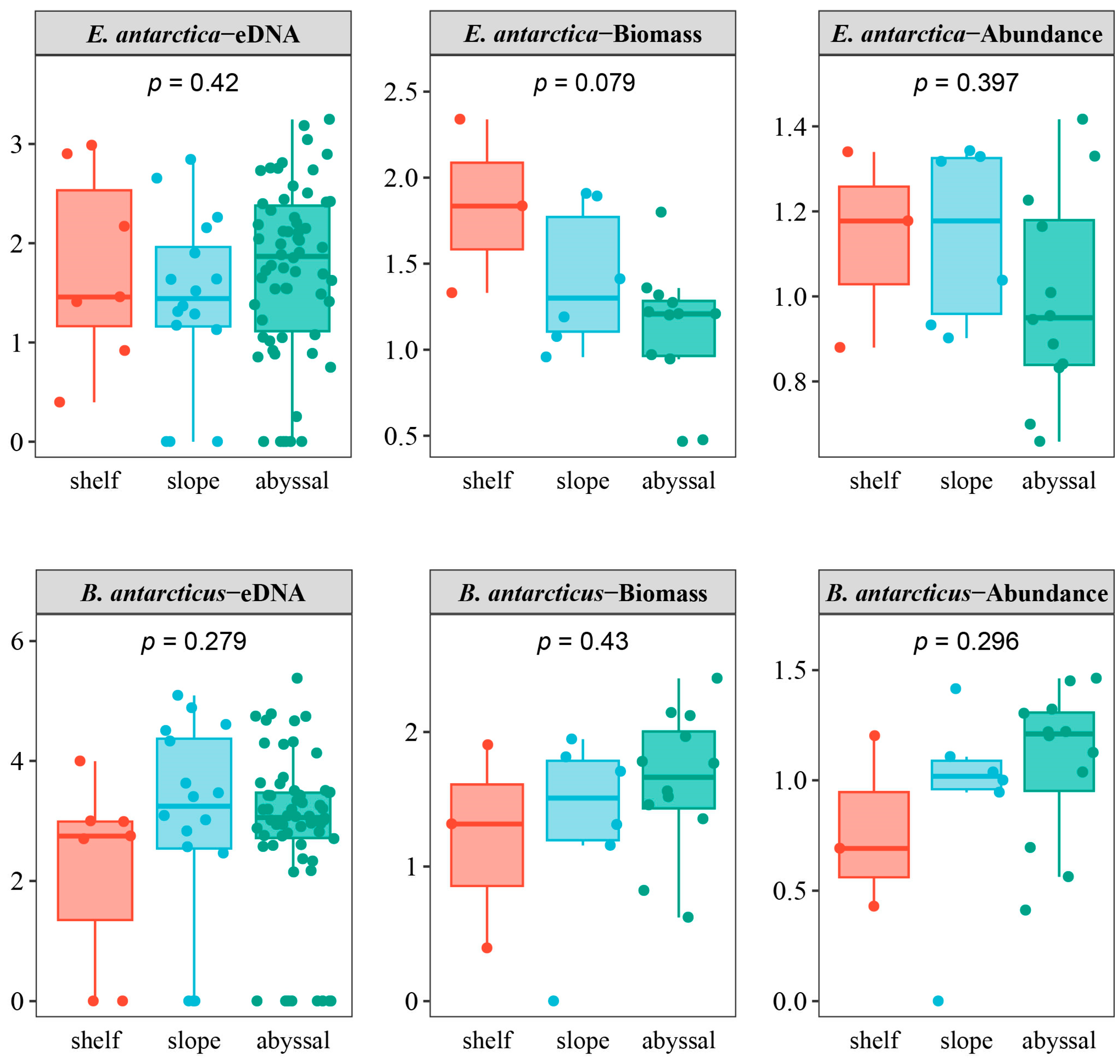
3.2. Comparison of Horizontal Distribution by eDNA and Trawling Methods

A total of 146 eDNA samples (78.1%) in 76 stations (89.4%) detected E. antarctica by qPCR, including 48 samples (77.4%) in 29 stations (90.6%) in 2021 (Figure 2(A1)) and 98 samples (78.4%) in 47 stations (88.7%) in 2022 (Figure 2(A2)). The station with the highest eDNA concentration was station C7′-05 in 2022 (5289 copies/L). No significant differences were observed in eDNA concentration between different stations (p > 0.05), whether analyzed annually or overall. A total of 519 specimens of E. antarctica were collected, of which 225 were collected in 2021, and 294 were collected in 2022 (Supplementary Table S2). The trawl survey showed that E. antarctica occurred at all stations (Figure 2(B1,B2)). The stations with the highest hourly abundance and hourly biomass were C4-11 in 2021 (25.1 inds/h) and CA1-10 in 2022 (217.2 g/h), respectively. No significant differences were observed in biomass or abundance between different stations (p > 0.05), whether analyzed annually or overall.
A total of 125 eDNA samples (66.8%) in 72 stations (84.7%) were found to be eDNA-positive for B. antarcticus, including 52 samples (83.9%) in 28 stations (87.5%) in 2021 (Figure 2(A3)) and 73 samples (58.4%) in 44 stations (83.0%) in 2022 (Figure 2(A4)). The number of samples found to be eDNA-positive for B. antarcticus was lower than that for E. antarctica. The station with the highest eDNA concentration was station C2′-08 in 2022 (35,690 copies/L). No significant differences were observed in eDNA concentration between different stations (p > 0.05), whether analyzed annually or overall. A total of 542 specimens of B. antarcticus were collected, of which 343 were collected in 2021, and 199 were collected in 2022 (Supplementary Table S2). Except for station C2′-06 in 2022, B. antarcticus were captured at all other stations (Figure 2(B3,B4)). The station with the highest hourly abundance and hourly biomass was CA2-05 in 2022 (249.5 inds/h and 28 g/h). No significant differences were observed in biomass or abundance between different stations (p > 0.05), whether analyzed annually or overall.
The eDNA concentration, fish biomass, and abundance of the two species were further compared between stations located at three different water depths (shelf, slope, and abyssal), as is shown in Figure 3. In the trawl surveys, the two fish species showed different distribution trends. E. antarctica tended to inhabit shallow waters, and their biomass and abundance gradually decreased with increasing water depth, with the highest in the continental shelf and the lowest in the abyssal areas. B. antarcticus, however, tended to inhabit deep-sea areas, and their biomass and abundance gradually increased with water depth, with the lowest on the continental shelf and the highest in the abyssal areas. The median eDNA concentration of E. antarctica was the highest in the abyssal areas, followed by the continental shelf and slope areas. Meanwhile, the mean eDNA concentration was the highest in the continental shelf (1.748), followed by the abyssal (1.730) and slope areas (1.429). The median eDNA concentration of B. antarcticus was the highest in the slope areas, followed by the abyssal and shelf areas. The mean eDNA concentrations were also the highest in the slope areas (2.993), followed by the abyssal (2.899) and shelf areas (2.204). However, all comparisons between the three kinds of stations were not significant.

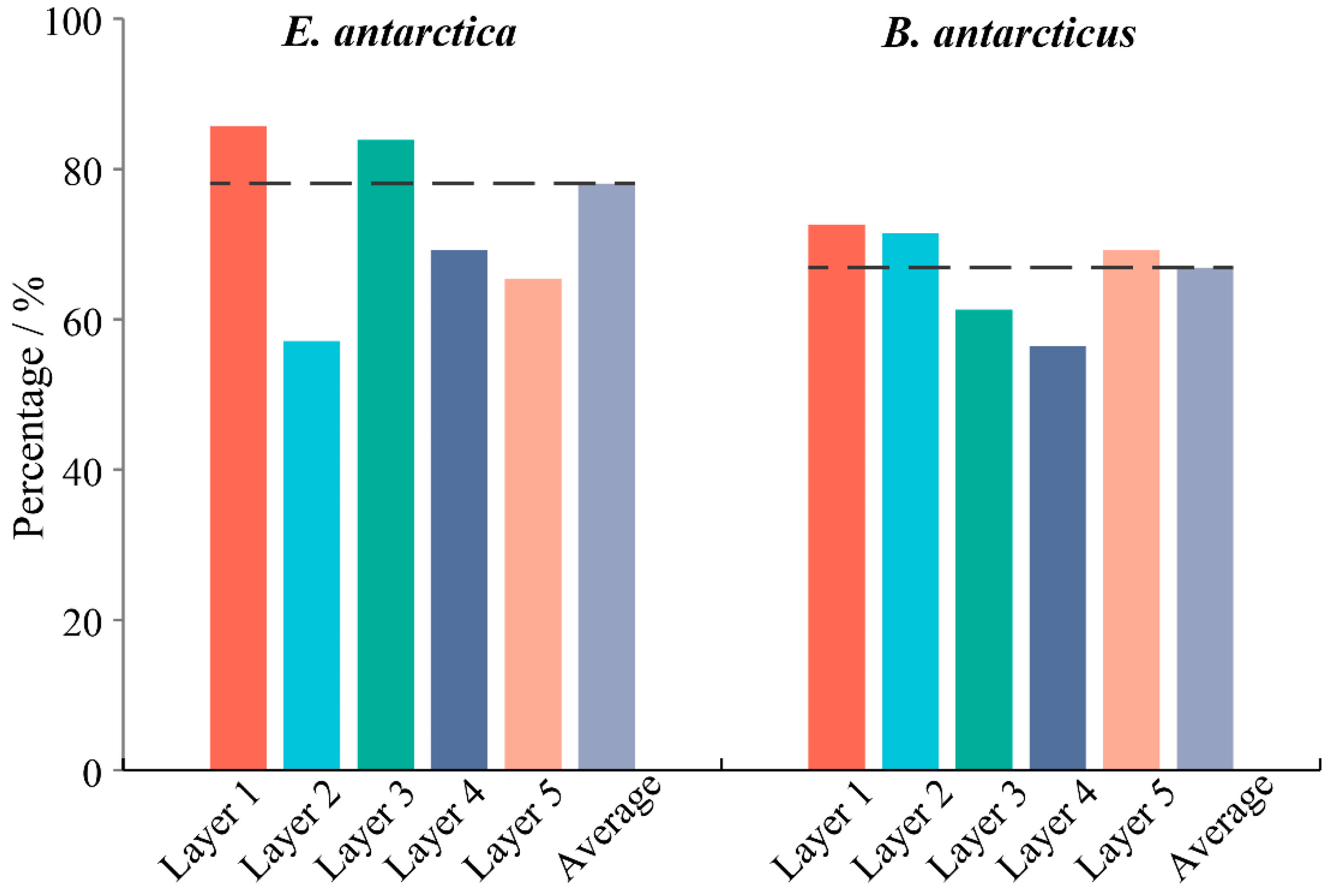
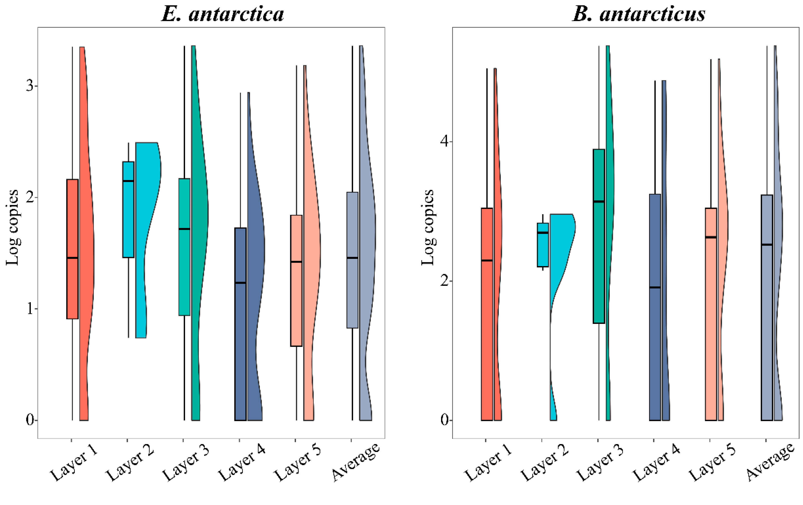
3.3. Comparison of Vertical Distribution by eDNA Method

The mean detection rate of E. antarctica was higher than that of B. antarcticus, with higher detection rates also observed in layers 1, 3, and 4. (Figure 4). However, the mean eDNA concentration of E. antarctica was lower than that of B. antarcticus (Figure 5). No significant difference was found in the eDNA detection rate or concentration among the layers for either E. antarctica or B. antarcticus.
For E. antarctica, the eDNA detection rates were found to be above the mean in layer 1 and layer 3, and correspondingly, the concentrations were also found to be above the mean in layer 1 and layer 3. In addition, layer 2 had the highest eDNA concentration, while it had the lowest detection rate. The lowest eDNA concentration occurred in layer 4, and the highest detection rate occurred in layer 1. The sample with the highest eDNA concentration was found in surface sampling at station C5′-00 in 2022.
For B. antarcticus, the eDNA detection rates were found to be higher than the mean in layer 1, layer 2, and layer 5, while the concentrations were found to be higher in layer 2, layer 3, and layer 5. The highest detection rate also occurred in layer 1, but the highest eDNA concentration occurred in layer 3. The lowest eDNA detection rate and concentration both occurred in layer 4. The sample with the highest eDNA concentration was found in bottom sampling at station C5′-05 in 2022.

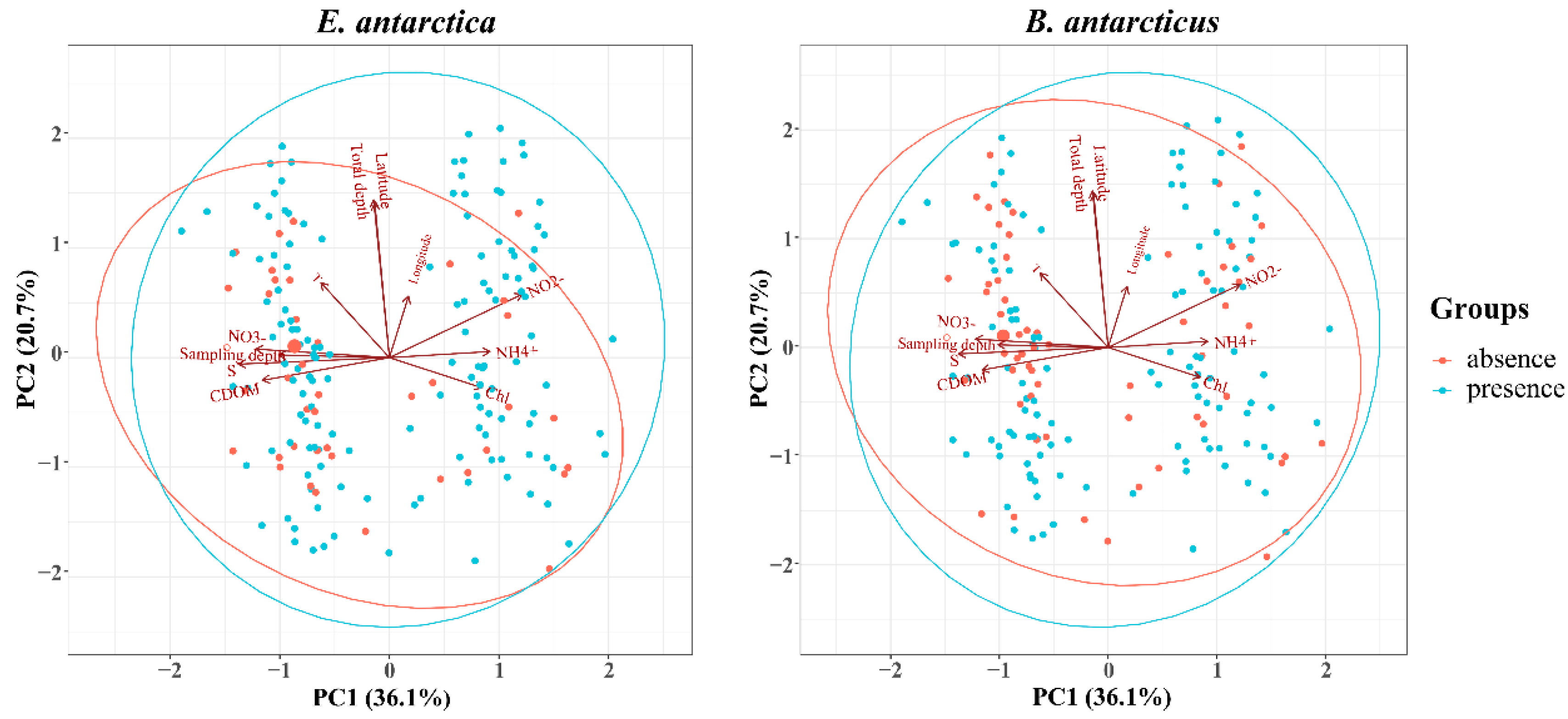
3.4. Environmental Factors Correlated with Distribution

Mantel’s test was employed to explore the correlation between the eDNA concentration, biomass, and abundance of two fish species and each environmental factor. The correlation test between four environmental factors (DO, PO43−, SiO32−, and distance from station to land) and eDNA and that between five environmental factors (total water depth, latitude, water temperature, CDOM, SiO32−, and distance from station to land) and biomass and abundance were excluded. No significant correlations were found between eDNA concentration or presence/absence and each environmental factor for either E. antarctica or B. antarcticus (Supplementary Figure S5). The biomass and abundance of E. antarctica were significantly correlated with chlorophyll, while the biomass and abundance of B. antarcticus were not correlated with each environmental factor (Supplementary Figure S6).
A GAM was used to assess whether environmental variables could predict eDNA concentration, eDNA presence/absence, biomass, and abundance in two fish species (Table 2). The optimal models between the logarithmic-transformed eDNA concentration of E. antarctica and various factors included NO3, longitude, chlorophyll, and NH4+. Among them, NO3 was the most important (12%) but was not significant, followed by longitude (9%). The optimal models between the logarithmic-transformed eDNA concentration of B. antarcticus and various factors included CDOM, chlorophyll, and latitude, among which CDOM was the most important (11.3%). The presence/absence of E. antarctica could be predicted by NO2, longitude, chlorophyll, sampling depth, and latitude, among which longitude was the most important (9.3%) but not significant. And the presence/absence of B. antarcticus could be predicted by temperature and total depth, among which temperature was the most important (11.1%). Chlorophyll can greatly predict the biomass of E. antarctica (93.2%). PO43− can effectively predict the abundance of E. antarctica and the biomass and abundance of B. antarcticus. Overall, the eDNA distribution of E. antarctica was related to nutrients, longitude, and chlorophyll, while the eDNA distribution of B. antarcticus was related to the physical environment. In the trawl survey, the biomass and abundance of the two fish species were related to chlorophyll and nutrients.
The remaining 11 environmental factors (total depth, sampling depth, longitude, latitude, temperature, salinity, CDOM, chlorophyll, NH4+, NO3, NO2) were used for PCA to explore the relationship between eDNA presence/absence and environmental factors (Figure 6). PC1 and PC2 explained 36.1% and 20.7% of the total variance, respectively. PC1 was mainly explained by nutrients, sampling depth, salinity, chlorophyll, and CDOM. PC2 was mainly explained by total depth, temperature, longitude, and latitude. As shown in Figure 6, the presence/absence groupings of E. antarctica and B. antarcticus detected by eDNA largely overlapped, indicating that environmental factors have little effect on the distribution of the two fish species.

4. Discussion

Here, we employed the traditional trawl survey and the eDNA method with a wider scope of investigation to assess the distribution patterns and resources of two typical mesopelagic fishes in the Cosmonaut Sea. Our results demonstrated the ability of eDNA to detect the distribution of mesopelagic fishes in the Southern Ocean.

4.1. The Horizontal Distribution Patterns of Antarctic Lanternfish and Antarctic Deep-Sea Smelt

Both species were detected at nearly all sampling stations, except for one station where B. antarcticus was not caught by trawling. There was no statistically significant difference in eDNA concentration, abundance, or biomass between these sampled stations, suggesting that the two species were widely distributed throughout the Cosmonaut Sea, with no evident aggregation areas. This is consistent with the results of many previous surveys on mesopelagic fishes. For example, the results of a fishery survey in the Cosmonaut Sea and Prydz Bay region during the “BROKE-West” campaign showed that the mesopelagic fishes were mainly concentrated in the oceanic zone [9], and the survey by Moteki et al. [10] also showed that the mesopelagic fish assemblages in the Lützow-Holm Bay (Cosmonaut Sea) were relatively uniform. Fishery surveys conducted in other areas of the Southern Ocean have also shown that the Antarctic lanternfish and Antarctic deep-sea smelt were evenly distributed in the oceanic zone, with no aggregation areas found [11,51,52,53].
Although both species are widely distributed throughout the Cosmonaut Sea, their habitat preferences differ. E. antarctica was found to prefer to inhabit shallow waters, with the highest mean eDNA concentration, biomass, and abundance found in the stations close to the continental shelf. B. antarcticus, on the contrary, showed a trend towards deep-sea distribution, with eDNA concentration, biomass, and abundance gradually increasing with increasing water depth. Studies have shown that E. antarctica prefer warmer offshore waters, and their distribution is related to Antarctic circumpolar deep water and less frequent in shelf areas [54]. However, our study challenges this view. Most surveys of mesopelagic fishes in the Southern Ocean have found that the water depth of the main habits of B. antarcticus is deeper than that of the habits of E. antarctica [7,9,11,53]. This suggests that water depth may be an important factor controlling the habitat preferences of the two species. Previous trawl surveys have also found more E. antarctica larvae distributed in shallow and offshore waters or in areas at the edge of the sea ice [12,13], while more B. antarcticus larvae have been found in deeper water [12,51], which may also contribute to the higher eDNA concentrations in the shelf area of E. antarctica and the slope area of B. antarcticus. Considering the effects of water currents that transport passive larvae away from their origin locations, the reasons why higher distributions of both larvae and adult fish were found in similar water depths deserve further investigation.
The higher biomass and abundance of E. antarctica in the nearshore and shallow waters of the Cosmonaut Sea may be partly related to the distributions of chlorophyll, as the biomass and abundance of E. antarctica were found to be significantly positively correlated with chlorophyll. Meanwhile, the Antarctic Slope Current, which exists in the coastal areas of the Cosmonaut Sea from east to west, was reported to play an important role in the distributions of krill, cetaceans, and chlorophyll through the early “BROKE” survey [55].

4.2. eDNA Reveals Different Vertical Distribution Structures in Two Fish Species

Notable, higher eDNA detection rates did not necessarily correspond to higher eDNA concentrations. For example, layer 2 (10–200 m) exhibited a high eDNA concentration of E. antarctica but had the lowest detection rate. Layer 3 (500 m) showed the highest eDNA concentration of B. antarcticus, while the eDNA detection rate there was lower than the mean value. These suggest that the vertical distribution of the genetic material is heterogeneous, with some genetic material clustering together while some does not. Aggregations of fish may release large amounts of eDNA within a given range, resulting in increased eDNA concentrations. However, detection at a given depth does not necessarily reflect real-time organism presence at that depth. Many particles containing eDNA are too large to remain suspended and are transported downward by gravity and settle to the seafloor, while the eDNA at the bottom was also found to be brought upward due to the mixing of tidal currents, upwelling, and some human activities [56]. This results in eDNA from fish living in specific waters appearing in other water layers. The surface layer showed the highest eDNA detection rate of B. antarcticus, while the eDNA concentration there was lower than the mean value. Exogenous eDNA contamination can lead to false positives and reduce the abundance of the target species [35]. We introduced negative controls at the laboratory stage to control contamination during the experiment, but no negative controls were collected during sampling due to logistical difficulties. Although several measures have been taken to reduce the risk of contamination during field sampling, the lack of sufficient negative controls could still have a potential impact on the results.
Despite this, the eDNA detection rate can still indicate that E. antarctica and B. antarcticus may occupy different vertical ecological niches, as the eDNA detection rates of E. antarctica were relatively high in the surface and 500 m layers compared to other layers, while the detection rates of B. antarcticus were relatively high in the surface, 200 m, and bottom layers. This is consistent with previous studies in the Cosmonaut Sea that found that E. antarctica was more commonly found in waters above 500 m, while B. antarcticus was found to have a more extensive vertical distribution with many of the fish being distributed in waters below 1000 m [9,10,57]. Similar vertical distribution patterns have also been well documented in other areas of the Southern Ocean, highlighting that B. antarcticus inhabits deeper water layers than E. antarctica [7,11,12,53,58].
The eDNA detection rate of E. antarctica is higher than that of B. antarcticus, which corresponds to the higher frequency of appearance of E. antarctica in trawl surveys, indicating a wider distribution. However, the mean eDNA concentration of E. antarctica is lower than that of B. antarcticus. Numerous studies have shown a positive correlation between eDNA concentration and biomass size [59,60,61], and the trawl results of this study also indicate that the biomass and abundance of B. antarcticus are higher. Therefore, E. antarctica may have a wider distribution, but the potential biomass of B. antarcticus may be higher in the Cosmonaut Sea. In addition, the actual biomass of B. antarcticus may still be underestimated as it usually inhabits deeper water than other mesopelagic fishes [62].

4.3. The Distribution of the Two Fish Species Is Affected by Different Environmental Factors

Mantel’s test revealed that there was no significant correlation between the eDNA concentration of the two fish species and each single environmental factor. This is reasonable as eDNA in the ocean may be affected by multiple environmental factors [37,63], resulting in an insignificant correlation between eDNA and a single environmental factor. The PCA of environmental factors also showed that the eDNA presence and absence groups were not well separated, indicating that the two fish species had strong environmental adaptability, which corresponded to their extensive distribution. At the same time, the PCA also indicated that factors other than environmental variables (like plankton and krill) may affect the distribution of the two fish species.
Based on the GAM, which can explore the effects of multiple environmental factors, we found that the biomass and abundance of both species were related to nutrients; specifically, the biomass of E. antarctica was greatly affected by chlorophyll, and abundance was affected by PO43− and NO3; the biomass and abundance of B. antarcticus were both affected by PO43−. Chlorophyll is related to the distribution of phytoplankton, while the concentrations of phosphorus and nitrogen in the ocean are affected by the death or predation of phytoplankton and zooplankton, which are primarily related to biological feeding activities [64,65]. These findings indicate that the distribution of the two species may be more affected by the availability of phytoplankton and zooplankton, which could serve as their food resources, as E. antarctica and B. antarcticus are widely recognized as opportunistic foragers that typically exploit a variety of prey resources in the food-scarce Southern Ocean [8,12]. Many studies on mesopelagic fishes showed that the distribution of E. antarctica was more affected by temperature [9,10,11,12], while our study highlighted the role of nutrients in affecting the distribution of E. antarctica and B. antarcticus. In the Cosmonaut Sea, the bait composition of E. antarctica mainly consists of copepods [8], and that of B. antarcticus consists of copepods and krill [66]. There is a certain degree of overlap in the feeding habits of the two species, and thus their spatial distributions may also overlap. However, the dietary composition of the two species may also differ in different marine areas, so the factors influencing their distribution in other marine areas need to be further investigated.
In contrast, the eDNA concentration and presence/absence of two fish species were related to different environmental factors; particularly, the eDNA concentration of B. antarcticus was primarily affected by physical environmental factors such as CDOM and latitude, while presence/absence was affected only by temperature and total water depth. This is reasonable because fish can actively swim to their target locations, potentially making biomass and abundance more closely related to nutrients, while eDNA, behaving like passive particles, is more likely to be affected by physical environmental factors, such as being transported by water currents. In addition, some environmental factors, such as salinity, pH, ultraviolet radiation, and temperature, can affect the degradation of eDNA [67,68,69]. Further investigation is thus needed to improve the assessment of fish biodiversity through the eDNA approach.

5. Conclusions

In this research, the eDNA and trawl approaches were employed to investigate the biogeographic patterns of two typical mesopelagic fishes in the Cosmonaut Sea in the Southern Ocean. The combined efforts of eDNA and trawl surveys have made it possible to conduct efficient and comprehensive biological research and monitoring in the remote and harsh environment of the Southern Ocean. Both approaches showed that the two species are widely distributed horizontally with no evident aggregation throughout the Cosmonaut Sea, but they differ in their vertical distribution structure, where Antarctic deep-sea smelt prefers deeper habitats, whereas Antarctic lanternfish tends to be more shallowly distributed. The biomass and abundance of both species from trawling samples were found to be more correlated with nutrients, indicating that the distribution of the two species may be more affected by food resources. In contrast, correlations between eDNA metrics and environmental factors were lower. Considering the possibility of genetic material being transported by water currents or degraded over time, models that can backtrack their trajectories are required to better understand the spatial and temporal distribution of fish species. Nevertheless, the eDNA approach still shows significant advantages for species detection in harsh environments, offering basic information to better understand the ecological characteristics of this polar region.

Supplementary Materials

The following supporting information can be downloaded at: https://www.mdpi.com/article/10.3390/fishes10070354/s1, Figure S1: Map of sampling stations divided into abyssal, slope and shelf stations. The left shows the sampling stations in 2021, and the right shows the sampling stations in 2022; Figure S2: qPCR amplification curve plot for plasmids from Electrona antarctica at different concentrations. The amplification information for each sample is shown in Supplementary Table S3; Figure S3: qPCR amplification curve plot for plasmids from Bathylagus antarcticus at different concentrations. The amplification information for each sample is shown in Supplementary Table S4; Figure S4: Plot of qPCR validation results for specific primers and probes. A, D are the qPCR amplification using E. antarctica and B. antarcticus as template, respectively; B, D are the qPCR amplification using five other Antarctic fish species and ultrapure water as templates; C, F are the qPCR amplification using eDNA collected from the Southern Ocean as template; Figure S5: Mantel’s test on the relationship between eDNA of two fish species and environmental factors. Ela represents E. antarctica, Baa represents B. antarcticus, Log represents the Log10 transformed eDNA concentration, 0/1 represents absence/presence; Figure S6: Mantel’s test on the relationship between biomass and abundance of two fish species and environmental factors. Ela represents E. antarctica, Baa represents B. antarcticus. SST represents sea surface temperature, DO represents dissolved oxygen; Table S1: Information on eDNA samples collection; Table S2: Information on RMT trawl survey; Table S3: qPCR amplification information for plasmids from Electrona antarctica at different concentrations; Table S4: qPCR amplification information for plasmids from Bathylagus antarcticus at different concentrations.

Author Contributions

Conceptualization, J.L., J.H. and Y.T.; Data curation, C.L.; Formal analysis, Y.W., C.L., M.D. and P.J.; Funding acquisition, Y.T.; Investigation, Y.W., P.J., W.Z., S.M. and J.L.; Methodology, Y.W. and J.L.; Resources, W.Z.; Supervision, J.H.; Visualization, C.L. and M.D.; Writing—original draft, Y.W.; Writing—review and editing, W.S. and Y.T. All authors have read and agreed to the published version of the manuscript.

Funding

This research was funded by the research project “Impact and Response of Antarctic Seas to Climate Change, IRASCC2020-2022” (Grant No. IRASCC 01-02-05C) from the Chinese Arctic and Antarctic Administration (CAA), Ministry of Natural Resources of the People’s Republic of China, the National Natural Science Foundation of China (42206085), and the Fundamental Research Funds for the Central Universities (No. 202261035).

Institutional Review Board Statement

The fish samples used in this study consisted of dead fish caught in the ocean, ensuring that there was no infliction of suffering or distress on the animals. We adhered to relevant ethical guidelines to respect and protect animal welfare throughout the research process.

Data Availability Statement

Data will be made available on request.

Acknowledgments

We thank the scientific staff and crew aboard the 37th and 38th Chinese National Antarctica Research Expeditions for their assistance with sampling. This work was financially supported by the research project “Impact and Response of Antarctic Seas to Climate Change, IRASCC2020-2022” (Grant No. IRASCC 01-02-05C) from the Chinese Arctic and Antarctic Administration (CAA), Ministry of Natural Resources of the People’s Republic of China, the National Natural Science Foundation of China (42206085), and the Fundamental Research Funds for the Central Universities (No. 202261035).

Conflicts of Interest

The authors declare that there are no conflicts of interest.

References

  1. Cherel, Y.; Ducatez, S.; Fontaine, C.; Richard, P.; Guinet, C. Stable isotopes reveal the trophic position and mesopelagic fish diet of female southern elephant seals breeding on the Kerguelen Islands. Mar. Ecol. Prog. Ser. 2008, 370, 239–247. [Google Scholar] [CrossRef]
  2. Smith, A.D.M.; Brown, C.J.; Bulman, C.M.; Fulton, E.A.; Johnson, P.; Kaplan, I.C.; Lozano-Montes, H.; Mackinson, S.; Marzloff, M.; Shannon, L.J.; et al. Impacts of fishing low–trophic level species on marine ecosystems. Science 2011, 333, 1147–1150. [Google Scholar] [CrossRef] [PubMed]
  3. Griffiths, S.P.; Olson, R.J.; Watters, G.M. Complex wasp-waist regulation of pelagic ecosystems in the Pacific Ocean. Rev. Fish Biol. Fish. 2013, 23, 459–475. [Google Scholar] [CrossRef]
  4. Irigoien, X.; Klevjer, T.A.; Røstad, A.; Martinez, U.; Boyra, G.; Acuña, J.L.; Bode, A.; Echevarria, F.; Gonzalez-Gordillo, J.I.; Hernandez-Leon, S.; et al. Large mesopelagic fishes biomass and trophic efficiency in the open ocean. Nat. Commun. 2014, 5, 3271. [Google Scholar] [CrossRef]
  5. Christiansen, H.; Dettai, A.; Heindler, F.M.; Collins, M.A.; Duhamel, G.; Hautecoeur, M.; Steinke, D.; Volckaert, F.A.; Van de Putte, A.P. Diversity of mesopelagic fishes in the Southern Ocean-a phylogeographic perspective using DNA barcoding. Front. Ecol. Evol. 2018, 6, 120. [Google Scholar] [CrossRef]
  6. Duan, M.; Ashford, J.R.; Bestley, S.; Wei, X.; Walters, A.; Zhu, G. Otolith chemistry of Electrona antarctica suggests a potential population marker distinguishing the southern Kerguelen Plateau from the eastward-flowing Antarctic Circumpolar Current. Limnol. Oceanogr. 2021, 66, 405–421. [Google Scholar] [CrossRef]
  7. Collins, M.A.; Stowasser, G.; Fielding, S.; Shreeve, R.; Xavier, J.C.; Venables, H.J.; Enderlein, P.; Cherel, Y.; Van de Putte, A. Latitudinal and bathymetric patterns in the distribution and abundance of mesopelagic fish in the Scotia Sea. Deep Sea Res. Part II Top. Stud. Oceanogr. 2012, 59, 189–198. [Google Scholar] [CrossRef]
  8. Duan, M.; Zhang, C.; Luo, Y.; Gao, L.; Liu, G.; Liu, C.; Sun, Y.; Li, J.; Ma, S.; Zhang, W.; et al. The feeding strategies of the antarctic lanternfish electrona antarctica (pisces: Myctophidae) in the amundsen and cosmonaut seas (Southern Ocean), assessed with a classification tree analysis. Polar Biol. 2024, 47, 515–532. [Google Scholar] [CrossRef]
  9. Van de Putte, A.P.; Jackson, G.D.; Pakhomov, E.; Flores, H.; Volckaert, F.A. Distribution of squid and fish in the pelagic zone of the Cosmonaut Sea and Prydz Bay region during the BROKE-West campaign. Deep Sea Res. Part II Top. Stud. Oceanogr. 2010, 57, 956–967. [Google Scholar] [CrossRef]
  10. Moteki, M.; Horimoto, N.; Nagaiwa, R.; Amakasu, K.; Ishimaru, T.; Yamaguchi, Y. Pelagic fish distribution and ontogenetic vertical migration in common mesopelagic species off Lützow-Holm Bay (Indian Ocean sector, Southern Ocean) during austral summer. Polar Biol. 2009, 32, 1461–1472. [Google Scholar] [CrossRef]
  11. Koubbi, P.; Hulley, P.-A.; Pruvost, P.; Henri, P.; Labat, J.-P.; Wadley, V.; Hirano, D.; Moteki, M. Size distribution of meso-and bathypelagic fish in the Dumont d’Urville Sea (East Antarctica) during the CEAMARC surveys. Polar Sci. 2011, 5, 195–210. [Google Scholar] [CrossRef]
  12. Flores, H.; Van de Putte, A.P.; Siegel, V.; Pakhomov, E.A.; Van Franeker, J.A.; Meesters, E.H.; Volckaert, F.A. Distribution, abundance and ecological relevance of pelagic fishes in the Lazarev Sea, Southern Ocean. Mar. Ecol. Prog. Ser. 2008, 367, 271–282. [Google Scholar] [CrossRef]
  13. Moteki, M.; Tsujimura, E.; Hulley, P.A. Developmental intervals during the larval and juvenile stages of the Antarctic myctophid fish Electrona antarctica in relation to changes in feeding and swimming functions. Polar Sci. 2017, 12, 88–98. [Google Scholar] [CrossRef]
  14. Lea, M.A.; Nichols, P.D.; Wilson, G. Fatty acid composition of lipid-rich myctophids and mackerel icefish (Champsocephalus gunnari)–Southern Ocean food-web implications. Polar Biol. 2002, 25, 843–854. [Google Scholar] [CrossRef]
  15. Murphy, E.; Watkins, J.; Trathan, P.; Reid, K.; Meredith, M.; Thorpe, S.; Johnston, N.; Clarke, A.; Tarling, G.; Collins, M.; et al. Spatial and temporal operation of the Scotia Sea ecosystem: A review of large-scale links in a krill centred food web. Philos. Trans. R. Soc. B Biol. Sci. 2007, 362, 113–148. [Google Scholar] [CrossRef]
  16. Saunders, R.A.; Hill, S.L.; Tarling, G.A.; Murphy, E.J. Myctophid fish (Family Myctophidae) are central consumers in the food web of the Scotia Sea (Southern Ocean). Front. Mar. Sci. 2019, 6, 530. [Google Scholar] [CrossRef]
  17. Gon, O. A description of the postlarva of Cygnodraco mawsoni Waite, 1916 (Pisces, Bathydraconidae), from the Southern Ocean. Afr. Zool. 1987, 22, 321–322. [Google Scholar]
  18. Goldsworthy, S.D.; Lewis, M.; Williams, R.; He, X.; Young, J.W.; Van den Hoff, J. Diet of Patagonian toothfish (Dissostichus eleginoides) around Macquarie Island, South Pacific Ocean. Mar. Freshw. Res. 2002, 53, 49–57. [Google Scholar] [CrossRef]
  19. McCormack, S.A.; Melbourne-Thomas, J.; Trebilco, R.; Blanchard, J.L.; Raymond, B.; Constable, A. Decades of dietary data demonstrate regional food web structures in the Southern Ocean. Ecol. Evol. 2021, 11, 227–241. [Google Scholar] [CrossRef]
  20. Saunders, R.A.; Collins, M.A.; Stowasser, G.; Tarling, G.A. Southern Ocean mesopelagic fish communities in the Scotia Sea are sustained by mass immigration. Mar. Ecol. Prog. Ser. 2017, 569, 173–185. [Google Scholar] [CrossRef]
  21. Freer, J.J.; Tarling, G.A.; Collins, M.A.; Partridge, J.C.; Genner, M.J. Predicting future distributions of lanternfish, a significant ecological resource within the Southern Ocean. Divers. Distrib. 2019, 25, 1259–1272. [Google Scholar] [CrossRef]
  22. Eastman, J.T.; Amsler, M.O.; Aronson, R.B.; Thatje, S.; McClintock, J.B.; Vos, S.C.; Kaeli, J.W.; Singh, H.; La Mesa, M. Photographic survey of benthos provides insights into the Antarctic fish fauna from the Marguerite Bay slope and the Amundsen Sea. Antarct. Sci. 2013, 25, 31–43. [Google Scholar] [CrossRef]
  23. Smith, J.; O’Brien, P.E.; Stark, J.S.; Johnstone, G.J.; Riddle, M.J. Integrating multibeam sonar and underwater video data to map benthic habitats in an East Antarctic nearshore environment. Estuar. Coast. Shelf Sci. 2015, 164, 520–536. [Google Scholar] [CrossRef]
  24. Yehui, W.; Chunlin, L.; Mi, D.; Chi, Z.; Zhenjiang, Y.; Yang, L.; Yongjun, T.; Jianfeng, H. Community structure of mesopelagic fauna and the length-weight relationships of three common fishes in the Cosmonaut Sea, Southern Ocean. Adv. Polar Sci. 2022, 33, 181–191. [Google Scholar]
  25. Valentini, A.; Taberlet, P.; Miaud, C.; Civade, R.; Herder, J.; Thomsen, P.F.; Bellemain, E.; Besnard, A.; Coissac, E.; Boyer, F.; et al. Next-generation monitoring of aquatic biodiversity using environmental DNA metabarcoding. Mol. Ecol. 2016, 25, 929–942. [Google Scholar] [CrossRef]
  26. Miya, M. Environmental DNA Metabarcoding: A novel method for biodiversity monitoring of marine fish communities. Annu. Rev. Mar. Sci. 2022, 14, 161–185. [Google Scholar] [CrossRef]
  27. Cowart, D.A.; Murphy, K.R.; Cheng, C.H.C. Metagenomic sequencing of environmental DNA reveals marine faunal assemblages from the West Antarctic Peninsula. Mar. Genom. 2018, 37, 148–160. [Google Scholar] [CrossRef]
  28. Liao, Y.; Miao, X.; Wang, R.; Zhang, R.; Li, H.; Lin, L. First pelagic fish biodiversity assessment of Cosmonaut Sea based on environmental DNA. Mar. Environ. Res. 2023, 192, 106225. [Google Scholar] [CrossRef]
  29. Zhang, Z.; Bao, Y.; Fang, X.; Ruan, Y.; Rong, Y.; Yang, G. A circumpolar study of surface zooplankton biodiversity of the Southern Ocean based on eDNA metabarcoding. Environ. Res. 2024, 255, 119183. [Google Scholar] [CrossRef]
  30. Taberlet, P.; Coissac, E.; Hajibabaei, M.; Rieseberg, L.H. Environmental DNA. Mol. Ecol. 2012, 21, 1789–1793. [Google Scholar] [CrossRef]
  31. Bohmann, K.; Evans, A.; Gilbert, M.T.P.; Carvalho, G.R.; Creer, S.; Knapp, M.; Yu, D.W.; De Bruyn, M. Environmental DNA for wildlife biology and biodiversity monitoring. Trends Ecol. Evol. 2014, 29, 358–367. [Google Scholar] [CrossRef]
  32. Stat, M.; John, J.; DiBattista, J.D.; Newman, S.J.; Bunce, M.; Harvey, E.S. Combined use of eDNA metabarcoding and video surveillance for the assessment of fish biodiversity. Conserv. Biol. 2019, 33, 196–205. [Google Scholar] [CrossRef]
  33. Wang, X.; Zhang, H.; Lu, G.; Gao, T. Detection of an invasive species through an environmental DNA approach: The example of the red drum Sciaenops ocellatus in the East China Sea. Sci. Total. Environ. 2022, 815, 152865. [Google Scholar] [CrossRef] [PubMed]
  34. Tsuji, S.; Takahara, T.; Doi, H.; Shibata, N.; Yamanaka, H. The detection of aquatic macroorganisms using environmental DNA analysis—A review of methods for collection, extraction, and detection. Environ. DNA 2019, 1, 99–108. [Google Scholar] [CrossRef]
  35. Miya, M.; Sato, Y.; Fukunaga, T.; Sado, T.; Poulsen, J.Y.; Sato, K.; Minamoto, T.; Yamamoto, S.; Yamanaka, H.; Araki, H.; et al. MiFish, a set of universal PCR primers for metabarcoding environmental DNA from fishes: Detection of more than 230 subtropical marine species. R. Soc. Open Sci. 2015, 2, 150088. [Google Scholar] [CrossRef] [PubMed]
  36. Harper, L.R.; Lawson Handley, L.; Hahn, C.; Boonham, N.; Rees, H.C.; Gough, K.C.; Lewis, E.; Adams, I.P.; Brotherton, P.; Phillips, S.; et al. Needle in a haystack? A comparison of eDNA metabarcoding and targeted qPCR for detection of the great crested newt (Triturus cristatus). Ecol. Evol. 2018, 8, 6330–6341. [Google Scholar] [CrossRef]
  37. Yu, Z.; Ito, S.-I.; Wong, M.K.-S.; Yoshizawa, S.; Inoue, J.; Itoh, S.; Yukami, R.; Ishikawa, K.; Guo, C.; Ijichi, M.; et al. Comparison of species-specific qPCR and metabarcoding methods to detect small pelagic fish distribution from open ocean environmental DNA. PLoS ONE 2022, 17, e0273670. [Google Scholar] [CrossRef]
  38. Yamamoto, S.; Minami, K.; Fukaya, K.; Takahashi, K.; Sawada, H.; Murakami, H.; Tsuji, S.; Hashizume, H.; Kubonaga, S.; Horiuchi, T.; et al. Environmental DNA as a ‘snapshot’ of fish distribution: A case study of Japanese jack mackerel in Maizuru Bay, Sea of Japan. PLoS ONE 2016, 11, e0149786. [Google Scholar]
  39. Qiao, Q.; Zhou, Q.; Wang, J.; Lin, H.J.; Li, B.Y.; Du, H.; Yan, Z.G. Environmental DNA reveals the spatiotemporal distribution and migration characteristics of the Yangtze Finless Porpoise, the sole aquatic mammal in the Yangtze River. Environ. Res. 2024, 263, 120050. [Google Scholar] [CrossRef]
  40. Liu, C.; Zhang, C.; Liu, Y.; Ye, Z.; Zhang, J.; Duan, M.; Tian, Y. Age and growth of Antarctic deep-sea smelt (Bathylagus antarcticus), an important mesopelagic fish in the Southern Ocean. Deep Sea Res. Part II Top. Stud. Oceanogr. 2022, 201, 105122. [Google Scholar] [CrossRef]
  41. Hunt, B.P.V.; Pakhomov, E.A.; Trotsenko, B.G. The macrozooplankton of the Cosmonaut Sea, east Antarctica (30 E–60 E), 1987–1990. Deep Sea Res. Part I Oceanogr. Res. Pap. 2007, 54, 1042–1069. [Google Scholar] [CrossRef]
  42. Lancraft, T.M.; Hopkins, T.L.; Torres, J.J.; Donnelly, J. Oceanic micronektonic/macrozooplanktonic community structure and feeding in ice covered Antarctic waters during the winter (AMERIEZ 1988). Polar. Biol. 1991, 11, 157–167. [Google Scholar] [CrossRef]
  43. Zu, Y.; Gao, L.; Guo, G.; Fang, Y. Changes of Circumpolar Deep Water between 2006 and 2020 in the south-west Indian Ocean, East Antarctica. Deep Sea Res. Part II Top. Stud. Oceanogr. 2022, 197, 105043. [Google Scholar] [CrossRef]
  44. Wang, Y.; Song, N.; Liu, S.; Chen, Z.; Xu, A.; Gao, T. DNA barcoding of fishes from Zhoushan coastal waters using mitochondrial COI and 12S rRNA genes. J. Oceanol. Limnol. 2023, 41, 1997–2009. [Google Scholar] [CrossRef]
  45. Ward, R.D.; Zemlak, T.S.; Innes, B.H.; Last, P.R.; Hebert, P.D. DNA barcoding Australia’s fish species. Philos. Trans. R. Soc. B Biol. Sci. 2005, 360, 1847–1857. [Google Scholar] [CrossRef]
  46. Wickham, H. ggplot2. Wiley Interdiscip. Rev. Comput. Stat. 2011, 3, 180–185. [Google Scholar] [CrossRef]
  47. Lê, S.; Josse, J.; Husson, F. FactoMineR: An R package for multivariate analysis. J. Stat. Softw. 2008, 25, 1–18. [Google Scholar] [CrossRef]
  48. R Core Team. R: A Language and Environment for Statistical Computing; R Foundation for Statistical Computing: Vienna, Austria, 2023; Available online: https://www.R-project.org/ (accessed on 28 January 2025).
  49. Wood, S.; Wood, M.S. Package ‘mgcv’, R package version 1.9-3; R Foundation for Statistical Computing: Vienna, Austria, 2015.
  50. Fox, J.; Weisberg, S.; Adler, D.; Bates, D.; Baud-Bovy, G.; Ellison, S.; Firth, D.; Friendly, M.; Gorjanc, G.; Graves, S.; et al. Package ‘car’, Version 3.1-3; R Foundation for Statistical Computing: Vienna, Austria, 2012.
  51. Hoddell, R.J.; Crossley, A.C.; Williams, R.; Hosie, G.W. The distribution of Antarctic pelagic fish and larvae (CCAMLR division 58.4.1). Deep Sea Res. Part II Top. Stud. Oceanogr. 2000, 47, 2519–2541. [Google Scholar] [CrossRef]
  52. Barrera-Oro, E. The role of fish in the Antarctic marine food web: Differences between inshore and offshore waters in the southern Scotia Arc and west Antarctic Peninsula. Antarct. Sci. 2002, 14, 293–309. [Google Scholar] [CrossRef]
  53. Moteki, M.; Koubbi, P.; Pruvost, P.; Tavernier, E.; Hulley, P.A. Spatial distribution of pelagic fish off Adélie and George V Land, East Antarctica in the austral summer 2008. Polar Sci. 2011, 5, 211–224. [Google Scholar] [CrossRef]
  54. Woods, B.L.; Van de Putte, A.P.; Hindell, M.A.; Raymond, B.; Saunders, R.A.; Walters, A.; Trebilco, R. Species distribution models describe spatial variability in mesopelagic fish abundance in the Southern Ocean. Front. Mar. Sci. 2023, 9, 981434. [Google Scholar] [CrossRef]
  55. Nicol, S.; Pauly, T.; Bindoff, N.L.; Strutton, P.G. “BROKE” a biological/oceanographic survey off the coast of East Antarctica (80–150° E) carried out in January–March 1996. Deep Sea Res. Part II Top. Stud. Oceanogr. 2000, 47, 2281–2297. [Google Scholar] [CrossRef]
  56. Jeunen, G.; Lamare, M.D.; Knapp, M.; Spencer, H.G.; Taylor, H.R.; Stat, M.; Bunce, M.; Gemmell, N.J. Water stratification in the marine biome restricts vertical environmental DNA (eDNA) signal dispersal. Environ. DNA 2020, 2, 99–111. [Google Scholar] [CrossRef]
  57. Duhamel, G.; Hulley, P.A.; Causse, R.; Koubbi, P.; Vacchi, M.; Pruvost, P.; Vigetta, S.; Irisson, J.O.; Mormede, S.; Belchier, M.; et al. Biogeographic patterns of fish. In Biogeographic atlas of the Southern Ocean; Scientific Committee on Antarctic Research: Cambridge, UK, 2014; pp. 328–362. [Google Scholar]
  58. Piatkowski, U.; Rodhouse, P.G.; White, M.G.; Bone, D.G.; Symon, C. Nekton community of the Scotia Sea as sampled by the RMT 25 during austral summer. Mar. Ecol. Prog. Ser. 1994, 112, 13–28. [Google Scholar] [CrossRef]
  59. Thomsen, P.F.; Kielgast, J.; Iversen, L.L.; Wiuf, C.; Rasmussen, M.; Gilbert, M.T.P.; Orlando, L.; Willerslev, E. Monitoring endangered freshwater biodiversity using environmental DNA. Mol. Ecol. 2012, 21, 2565–2573. [Google Scholar] [CrossRef]
  60. Doi, H.; Inui, R.; Akamatsu, Y.; Kanno, K.; Yamanaka, H.; Takahara, T.; Minamoto, T. Environmental DNA analysis for estimating the abundance and biomass of stream fish. Freshw. Biol. 2017, 62, 30–39. [Google Scholar] [CrossRef]
  61. Yamamoto, S.; Masuda, R.; Sato, Y.; Sado, T.; Araki, H.; Kondoh, M.; Minamoto, T.; Miya, M. Environmental DNA metabarcoding reveals local fish communities in a species-rich coastal sea. Sci. Rep. 2017, 7, 40368. [Google Scholar] [CrossRef] [PubMed]
  62. Pusch, C.; Hulley, P.A.; Kock, K.H. Community structure and feeding ecology of mesopelagic fishes in the slope waters of King George Island (South Shetland Islands, Antarctica). Deep. Sea Res. Part I Oceanogr. Res. Pap. 2004, 51, 1685–1708. [Google Scholar] [CrossRef]
  63. Harrison, J.B.; Sunday, J.M.; Rogers, S.M. Predicting the fate of eDNA in the environment and implications for studying biodiversity. Proc. R. Soc. B Biol. Sci. 2019, 286, 20191409. [Google Scholar] [CrossRef]
  64. Conley, D.J.; Paerl, H.W.; Howarth, R.W.; Boesch, D.F.; Seitzinger, S.P.; Havens, K.E.; Lancelot, C.; Likens, G.E. Controlling eutrophication: Nitrogen and phosphorus. Science 2019, 323, 1014–1015. [Google Scholar] [CrossRef]
  65. Boyce, D.G.; Lewis, M.R.; Worm, B. Global phytoplankton decline over the past century. Nature 2010, 466, 591–596. [Google Scholar] [CrossRef]
  66. Liu, C.; Zhang, C.; Wang, Y.; Duan, M.; Zhu, Y.; Zhang, W.; Li, J.; Ma, S.; Ju, P.; Shi, W.; et al. Ontogenetic shift in feeding habits of Antarctic deep-sea smelt Bathylagus antarcticus in the Cosmonaut Sea, East Antarctica. Polar Biol. 2025, 48, 25. [Google Scholar] [CrossRef]
  67. Andruszkiewicz, E.A.; Koseff, J.R.; Fringer, O.B.; Ouellette, N.T.; Lowe, A.B.; Edwards, C.A.; Boehm, A.B. Modeling environmental DNA transport in the coastal ocean using Lagrangian particle tracking. Front. Mar. Sci. 2019, 6, 477. [Google Scholar] [CrossRef]
  68. Murakami, H.; Yoon, S.; Kasai, A.; Minamoto, T.; Yamamoto, S.; Sakata, M.K.; Horiuchi, T.; Sawada, H.; Kondoh, M.; Yamashita, Y.; et al. Dispersion and degradation of environmental DNA from caged fish in a marine environment. Fish. Sci. 2019, 85, 327–337. [Google Scholar] [CrossRef]
  69. Tzafesta, E.; Shokri, M. The combined negative effect of temperature, UV radiation and salinity on eDNA detection: A global meta-analysis on aquatic ecosystems. Ecol. Indic. 2025, 176, 113669. [Google Scholar] [CrossRef]
Figure 1. A map of eDNA and midwater trawl sampling stations in the Cosmonaut Sea. The upper portion shows the sampling stations in 2021, and the lower portion shows the sampling stations in 2022.
Fishes 10 00354 g001
Figure 2. The horizontal distribution of E. antarctica and B. antarcticus in the Cosmonaut Sea. (A1,A2) represent the eDNA concentrations of E. antarctica in 2021 and 2022, respectively. (A3,A4) represent the eDNA concentrations of B. antarcticus in 2021 and 2022, respectively. eDNA concentration is represented by logarithmic-transformed copies. (B1,B2) represent the abundance and biomass standardized as an hour trawl of E. antarctica in 2021 and 2022, respectively. (B3,B4) represent the abundance and biomass standardized as an hour trawl of B. antarcticus in 2021 and 2022, respectively.
Fishes 10 00354 g002
Figure 3. A comparison of the eDNA concentration, biomass, and abundance of E. antarctica and B. antarcticus between shelf, slope, and abyssal stations. eDNA concentration is represented by logarithmic-transformed copies. Biomass and abundance are standardized as an hour trawl and logarithmic-transformed. Each box plot presents the p-value of the overall differences obtained from the Kruskal–Wallis test. The horizontal line in the middle of the box plot represents the median value.
Fishes 10 00354 g003
Figure 4. A comparison of eDNA detection rates between E. antarctica and B. antarcticus in different water layers. The bars represent the proportion of fish species detected with respect to the total sample in the corresponding layers. The dashed line represents the mean detection rate.
Fishes 10 00354 g004
Figure 5. A comparison of eDNA concentration between E. antarctica and B. antarcticus in different water layers. The left box represents the eDNA copies of two fish in each layer, while the right kernel density represents sample abundance. eDNA concentration is represented by logarithmic-transformed copies.
Fishes 10 00354 g005
Figure 6. Principal Component Analysis (PCA) of environmental factors of 187 samples in 85 sampling stations, with ellipse showing 95% confidence interval. We group presence (blue) and absence (red) of eDNA using different colors and circles.
Fishes 10 00354 g006
Table 1. Species-specific qPCR primers and probes used in this study.
SpeciesOligo SequencesAssay PerformanceAmplicon Length
E. antarcticaForward: 5′-CCCTATTTGTCTGAGCCGTCCTC-3′PCR efficiency: 98.32%
R2 = 0.9995
LOD: 8
LOQ: 14
107 bp
Reverse: 5′-GGTGTTTAGGTTCCGGTCCGTTAA-3′
Probe: 5′FAM-TGCTCCTCTCACTCCCTGTACTAGCTGCCG-3′BHQ1
B. antarcticusForward: 5′-CATGCAGGAGCTTCCGTAGAC-3′PCR efficiency: 90.60%
R2 = 0.9993
LOD: 12
LOQ: 18
153 bp
Reverse: 5′-GACAGACCAAATAAAGAGGGGAGTC-3′
Probe: 5′FAM-ACCATCTTCTCCCTCCACCTCGCTGGG-3′BHQ1
Table 2. GAM (Generalized Additive Model) analysis for relationship between distribution of two fish species and environmental factors.
Explanatory VariableAccumulation of
Deviance Explanation/%
Importance/%pAIC (Akaike Information Criterion)
Log—E. antarcticaNO312120.28 493.8053
Longitude21.69.6<0.05484.9752
Chl24.63<0.01480.255
Salinity25.71.1<0.05478.748
NH4+271.30.10 477.5129
0/1—E. antarcticaNO23.63.60.09 197.7437
Longitude12.99.30.06 193.4223
Chl17.64.70.19 191.4463
sampling depth19.92.30.06 189.6297
Latitude21.71.80.27 188.7583
Biomass—E. antarcticaChl93.293.2<0.01184.7565
DO1006.8<0.0138.87483
Abundance—E. antarcticaPO48080<0.01125.6865
NO399.419.4<0.0168.78184
Log—B. antarcticusCDOM11.311.3<0.01699.667
Chl153.7<0.01693.4619
Latitude17.92.90.31 692.783
0/1—B. antarcticusT11.111.1<0.01234.8247
total depth197.9<0.01224.4735
Biomass—B. antarcticusPO445.445.4<0.01232.3302
NO357.712.3<0.01230.5606
Abundance—B. antarcticusPO463.563.5<0.01142.2869
NH4+72.89.3<0.01138.3001
Log indicates the Log10-transformed eDNA concentration. 0/1 indicates absence/presence.
Disclaimer/Publisher’s Note: The statements, opinions and data contained in all publications are solely those of the individual author(s) and contributor(s) and not of MDPI and/or the editor(s). MDPI and/or the editor(s) disclaim responsibility for any injury to people or property resulting from any ideas, methods, instructions or products referred to in the content.

