Limit Reference Points and Equilibrium Stock Dynamics in the Presence of Recruitment Depensation

Abstract

Depensation (or an Allee effect) has recently been detected in stock–recruitment relationships (SRRs) in four Atlantic herring stocks and one Atlantic cod stock using a Bayesian statistical approach. In the present study, we define the Allee effect threshold (B_AET) for these five stocks and propose B_AET as a candidate limit reference point (LRP). We compare B_AET to traditional LRPs based on proportions of equilibrium unfished biomass (B₀) and biomass at maximum sustainable yield (B_MSY) assuming a Beverton–Holt or Ricker SRR with and without depensation, and to the change point from a hockey stick SRR (B_CP). The B_AET for the case studies exceeded 0.2 B₀ and 0.4 B_MSY for three of the case study stocks and exceedances of 0.2 B₀ were more common when the Ricker form of the SRR was assumed. The B_AET estimates for all case studies were less than B_CP. When there is depensation in the SRR, multiple equilibrium states can exist when fishing at a fixed fishing mortality rate (F) because the equilibrium recruits-per-spawner line at a given F can intersect the SRR more than once. The equilibrium biomass is determined by whether there is excess recruitment at the initial projected stock biomass. Estimates of equilibrium F_MSY in the case studies were generally higher for SRRs that included the depensation parameter; however, the long-term F that would lead the stock to crash (F_crash) in the depensation SRRs was often about half the F_crash for SRRs without depensation. When warranted, this study recommends exploration of candidate LRPs from depensatory SRRs, especially if Allee effect thresholds exceed commonly used limits, and simulation testing of management strategies for robustness to depensatory effects.

1. Introduction

Scientific advice for fisheries management typically involves the estimation of biological reference points defined in terms of stock biomass (B) and/or fishing mortality rate (F) (e.g., [1,2,3,4]). Fishery management goals generally have a stock approach or fluctuate around a target reference point and to avoid breaching a limit reference point (LRP) [5]. Biological reference points are used to assign stock status, are used as thresholds in the evaluation of the performance of management strategies, and also serve as triggers for rebuilding plans (e.g., [3,6,7]). The LRP in Canadian policy is defined as a threshold to avoid serious harm to the productivity of the stock and is generally defined in terms of either total biomass, spawning stock biomass (SSB), abundance, or a proxy for these [1]. Other jurisdictions define similar reference points (e.g., a minimum stock size threshold in the USA [8]; the biomass limit below which a stock is considered to have reduced reproductive capacity or B_lim [2]). A common interpretation of an LRP is a biomass threshold to avoid recruitment overfishing (e.g., [9]) or the biomass below which recruitment reduces with SSB (e.g., [2]). It is difficult to define such a threshold until a stock has fallen below that point [10,11], so generic policy default LRPs and rules of thumb are commonly used in practice (e.g., 0.4 B_MSY in Canada [1]; 0.5 B_MSY in the USA [3]; 0.2 B₀ in Australia and New Zealand [4,7].

A demographic Allee effect (hereafter Allee effect; [12]), in contrast to compensatory assumptions, occurs when the per capita population growth rate decreases as population abundance declines, and can stunt population recovery [13]. Allee effects are commonly referred to as depensation in fisheries science (e.g., [14]) and are consistent with the definition of serious harm in Canadian Policy [15]. There has been limited evidence of Allee effects in marine fish populations reported in the literature. For example, Myers et al. [16] detected a significant Allee effect in only 3 of 128 stock–recruitment relationships (SRRs) using a likelihood ratio test between SRR models with and without a depensation parameter. Liermann and Hilborn [17] similarly found little evidence for depensation in the same data set. Hilborn et al. [18] repeated the Myers et al. [16] analysis with 15 more years of additional data from the (Ransom A. Myers) RAM Legacy database [19] and only found significant depensation in 4 of 113 stocks when looking at the relationship between recruitment and biomass and in 8 of 109 stocks when looking at the relationship between surplus production and biomass. A separate analysis of the RAM database by Keith and Hutchings [20] that looked at the ratio of recruits to SSB vs. SSB across 104 species also yielded little evidence of Allee effects, with the exception of Atlantic cod (Gadus morhua). The ability to detect significant Allee effects in SRRs requires data at low population sizes [18,21,22] and the early statistical evaluations of data suffered from low statistical power [20]. Significant Allee effects were recently reported using Bayesian statistical methods in the estimation of SRR parameters in four of nine Atlantic herring (Clupea harengus) stocks in the Northeast Atlantic [21] and for the St. Pierre Bank (3Ps) Atlantic cod stock [22].

LRPs have been defined for 102 of Canada’s major fish stocks [23]. The most commonly used approach for defining LRPs for these stocks was the policy default (0.4 B_MSY or a proxy for this). While the potential for Allee effects has been acknowledged in the selection of LRPs for some Canadian stocks (e.g., Pacific herring, Clupea pallasii [15]), LRPs in Canada have not been selected based on estimated Allee effect thresholds [23]. National guidelines for defining LRPs or equivalent reference points (e.g., B_lim or “hard limits” in New Zealand’s harvest strategy standard) do not currently consider Allee effect thresholds (e.g., [2,4]). Perälä et al. [22] calculated 95% central probability intervals for an “Allee effect threshold” (defined by the authors as the inflection point in the SRR) for the 3Ps Atlantic cod stock in southern Newfoundland from two different SRRs, which included a depensation parameter. The LRP that is formally used to provide scientific advice for this stock was defined based on a break-point analysis to identify the biomass above which recruitment increases with increasing biomass [24] and was below the 95% central probability interval of the Allee effect threshold for both SRRs [22].

In this study, we evaluate candidate LRPs for the five stocks which have been identified recently in the literature [21,22] to have significant depensation in their SRRs. The specific objectives of this study were (i) to identify a candidate LRP as a threshold below which there is depensation in the SRR and to compare it to commonly used LRPs based on proportions of B₀ or B_MSY and approaches to define B_lim [2] and (ii) to evaluate the effect of depensation in SRRs on equilibrium reference points.

2. Materials and Methods

2.1. Data

The five case study stocks evaluated in this study were four Atlantic herring stocks—Bothnian Sea (BS), Gulf of Riga (GoR), North Sea autumn spawners (NSAS), and Western Baltic spawning spawners (WBSS)—and one Atlantic cod stock: Northwest Atlantic Fisheries Organization (NAFO) subdivision 3Ps. The model-estimated SSB, recruitment, selectivity, and fixed model inputs of natural mortality rate (M)-at-age, weight-at-age, and maturity-at-age for the herring stocks were obtained from ICES stock assessment reports [25,26] and stock assessment outputs (stockassessment.org). The model-estimated SSB, recruitment, selectivity, and M-at-age and the fixed model inputs of weight-at-age and maturity-at-age for the 3Ps cod stock were obtained from [22,24,27]. The NSAS and BS herring stocks used a stochastic state-space model [28], the WBSS and GR herring stocks used a virtual population analysis approach using Extended Survivors Analysis [29], and the 3Ps cod stock used an integrated state-space model [27]. Although the SSB and recruitment values for each stock are estimated, these models did not assume an underlying SRR. While there are potential issues with interpreting stock assessment estimates as independent observations for post hoc analyses [30,31], the intent of this study is to describe the effect of depensation on equilibrium reference point calculations, as inferred from recent stock assessments and reference point estimates are not intended for management purposes. The SRRs for the case studies have been previously published [21,22]. Inferences in the present study are conditional on the estimation models used for these stocks, and should be updated as new information becomes available.

2.2. Stock–Recruitment Models

Recruitment was modeled as a function of SSB using the Beverton–Holt (BH; [32]) and Ricker [33] models as well as extensions of these two models that include an additional depensation parameter, the sigmoid BH (sBH; [16]), and the Saila–Lorda (SL; [34,35]), respectively. Various parameterizations of a 2-parameter or 3-parameter BH and Ricker models have been described (e.g., [16,36,37]); however, we used the parameterizations from Perälä et al. [22] with recruitment ($R_i$) in year i as a function of SSB ($B_i):$

$$\mathrm{sBH}: R_i = {\displaystyle \frac{R_{\infty }}{1+{\left(B_{50}/B_i\right)}^c}}$$

(1)

where $R_{\infty }$ is the asymptotic recruitment, $B_{50}$ is the model predicted SSB at 50% of $R_{\infty }$ and $c$ is the depensation parameter, and

$${\mathrm{SL}: R}_i = k{\left({\displaystyle \frac{B_i}{B_k}}\right)}^c{e}^{c\left(1 - B_i/B_k\right)}$$

(2)

where $k$ is the maximum predicted recruitment, $B_k$ is the SSB at maximum predicted recruitment, and $c$ is the depensation parameter. When $c$ ≤ 1 in Equations (1) and (2), there is compensation at all stock sizes in the SRR, and when $c$ > 1, there is depensation in the SRR below some biomass value. When $c$ = 1, Equations (1) and (2) reduce to the traditional compensatory BH and Ricker models. The SRR model parameters were estimated using the Bayesian approach described in Perälä and Kuparinen [21] using the R package rstan version 2.32.7 [38] that provides the posterior probability distribution of the model parameters given priors for each parameter and a likelihood function that assumes that recruitment is lognormally distributed with the location parameter ${\mu }_i = \ln \left(E\left(R_i\right)\right) - 0.5{\sigma }^2$ and scale parameter $\sigma$. Ten thousand iterations were used, with one thousand iterations for warm-up for each of four Markov chains. Convergence of the models was confirmed visually from Markov chain trace plots, confirming $\widehat{R}$ values (comparing the between- and within-chain estimates for model parameters) were near 1 and less than 1.02 using the R package shinystan version 2.6.0 [39]. Divergent chains were observed in some model fits using the default stan settings so ‘adapt_delta’ was increased 0.99 and ‘max_treedepth’ was increased to 12 to achieve convergence following the guidance in the Stan user manual [40]. Similarly to the approach used by Perälä and Kuparinen [21], priors for the recruitment model parameters ($R_{\infty }$ or $k$) and SSB model parameters ($B_{50}$ or $B_k$) were defined as uniform distributions with lower limits of zero and upper limits as the maximum recruitment or SSB in the time series, and the prior for $\sigma$ was set as a uniform distribution between 0 and 2. The prior for the $c$ parameter was defined as a two-parameter sigmoidal function, defined by Perälä and Kuparinen [21], that effectively represents a differentiable step function over the range of 0 to 5 with equal density for $c$ < 1 and $c$ > 1 (i.e., equal a priori weight for compensation and depensation). The upper limits of the uniform distributions for the recruitment model parameters ($R_{\infty }$ or $k$) and SSB model parameters ($B_{50}$ or $B_k$) for the 3Ps cod stock were increased to twice the maximum observed recruitment or SSB, consistent with the priors used by Perälä et al. [22]. This was necessary because a maximum recruitment (SL model) or asymptotic recruitment (sBH model) appear to occur at a value greater than the maximum observed SSB in the stock–recruit data set (Figure 1). The reported SRR parameters were the median values from the posterior. The BH and Ricker model parameter estimates were obtained using the same priors and likelihood as the sBH and SL models, respectively, but fixing the $c$ parameter in Equations (1) and (2). Uncertainty in predicted recruitment from the SRR models was quantified using 90% credible intervals calculated from the posterior distribution of model parameters evaluated across the range of historical SSB values.

Model selection comparisons were conducted using a leave-one-out cross-validation information criterion (LOOIC; [41]) for Bayesian models using Pareto smoothed importance sampling using the R package loo version 2.8.0 [42]. Leave-one-out cross-validation is a method of estimating pointwise out-of-sample prediction accuracy from a Bayesian model using the log-likelihood evaluated at the posterior simulations of the parameter values [41]. The LOOIC was used for the model selection comparisons in the same way as other commonly used information criteria such as Akaike information criterion [43], such that given a set of models fit to the same data, the model with the minimum value is preferred.

2.3. Traditional Reference Points

The equilibrium unfished SSB (B₀) and the equilibrium SSB at maximum sustainable yield (B_MSY) were calculated to obtain traditional reference points of 0.2 B₀ and 0.4 B_MSY. The vectors of selectivity-at-age ($v_a$), M-at-age ($M_a$), weight-at-age ($w_a$), and maturity-at-age ($m_a$) were defined as the mean values-at-age from the last five years of the assessment for each stock. The B₀ and equilibrium unfished recruitment (R₀) were calculated as the SSB and predicted recruitment at the intersection of the SRR and the unfished equilibrium recruits-per-spawner (R/S) line (i.e., replacement line). The unfished replacement line was defined as a line through the origin with a slope equal to the inverse of the unfished SSB-per-recruit (${\phi }_0$), where the SSB-per-recruit for a given F is as below:

$${\phi }_F = {\displaystyle {\sum }_{a = a_{rec}}^{{a = a}_{max}}}\left(l_a{w}_a{m}_a\right)$$

(3)

where $a_{rec}$ is the age at recruitment and where $a_{max}$ is the maximum age (plus group), and $l_a$ is the survivorship-at-age defined as follows:

$$l_a = \left\{\begin{array}{cc}1, & a = a_{rec}\\ l_{a - 1}{e}^{ -(M_{a - 1} + F{v}_{a - 1})}, & a_{rec} < a < a_{max}\\ {\displaystyle \frac{l_{a - 1}{e}^{ -(M_{a - 1} + F{v}_{a - 1})}}{1 - e^{ -(M_{a - 1} + F{v}_{a - 1})}}}, & a = a_{max}\end{array}\right.$$

(4)

B_MSY was estimated as the equilibrium biomass from fishing long-term at F_MSY. F_MSY was estimated numerically as the F that provides a maximum yield over a range of F values where yield was calculated as the product of the equilibrium yield-per-recruit (${YPR}_F$) and the equilibrium number of recruits ($R_F$) from fishing at a specified F where

$${YPR}_F = {\displaystyle {\sum }_{a = a_{rec}}^{{a = a}_{max}}}{l}_a{w}_a{\displaystyle \frac{F{v}_a\left(1 - e^{ -(M_a + F{v}_a)}\right)}{M_a + F{v}_a}}$$

(5)

and $R_F$ is the recruitment at the intersection of the SRR and the replacement line at the corresponding F (i.e., a line through the origin with a slope equal to the inverse of ${\phi }_F$). The equilibrium B_MSY was then estimated as the product of ${\phi }_F$ and $R_F$ evaluated at F_MSY. The F that results in the population going extinct in the long-term under equilibrium conditions was defined as F_crash (the minimum F > 0 for which the equilibrium SSB is zero).

When an SRR is monotonically increasing and the concavity does not change (e.g., BH model), the replacement line with the slope 1/${\phi }_F$ intersects the SRR once and the yield curve is dome-shaped [44]. For some of the SRR fits (e.g., three parameter models such as the sBH and SL), a replacement line can intersect the SRR more than once ([36]; e.g., Figure 2). These intersection points were identified by substituting $B_i$ in Equations (1) and (2) with ${\phi }_F{R}_i$ (i.e., ${\phi }_F{=B_i/R}_i$ = SSB-per-recruit) and identifying the $R_i$ values of the intersection points using the uniroot.all function in the rootSolve R package version 1.8.2.3 [45]. The corresponding $B_i$ values of the intersection points were identified by solving Equations (1) and (2) for $B_i$ given $R_i$ and represent thresholds for excess recruitment (Figure 2) where excess recruitment is the recruitment that exceeds the replacement line [46].

The change point in a hockey stick (HS) SRR was defined as B_CP and is consistent with the ICES description of B_lim for stock Type 2 (stocks with a wide dynamic range of SSB, and evidence that recruitment is or has been impaired) in ICES [2]. The change point was estimated following the methods of Barrowman and Myers [47] using maximum-likelihood estimation assuming a lognormal error distribution. The HS model is as follows:

$$R_i = \alpha \min \left(B_i,B_{CP}\right)$$

(6)

where the parameter $\alpha$ is the slope of the linear regression portion of the curve and the parameter B_CP is the change point in SSB from the linear regression portion of the curve to the horizontal line portion of the curve [47]. The HS model was only used to estimate B_CP as a candidate LRP and other reference point estimates (e.g., B₀, B_MSY) were not estimated from the HS model. An HS model did not fit the 3Ps cod data so B_CP was defined as the highest observed SSB, consistent with the description of B_lim for stock Type 3 (stocks with a wide dynamic range of SSB, and evidence that recruitment is or has been impaired, with no clear asymptote in recruitment at high SSB) in ICES [2] to facilitate comparisons to the other reference points. All computations and statistical analyses were conducted using R version 4.4.3 [48] and the R scripts and the data for all analyses can be obtained from github (https://github.com/z5a1n/LRP_depensation).

2.4. Allee Effect Reference Points

Three reference points were defined from the sBH and SL models. Following Hutchings [13], the Allee threshold (B_AT) was defined as the theoretical biomass at which the realized per capita population growth rate is zero and the Allee effect threshold (B_AET) as the biomass where the per capita population growth rate declines with declining biomass. The logarithm of the per capita recruitment, ln(R/SSB), was used as a proxy for the realized per capita population growth rate, with B_AET estimated as the SSB at the maximum ln(R/SSB), and B_AT estimated as the SSB at which ln(R/SSB) equals the ln(R/SSB) at B₀ (Figure 3). A B_AT greater than zero is indicative of a “strong Allee effect”, in contrast to a “weak Allee effect”, where the SSB at which ln(R/SSB) equals the ln(R/SSB) at B₀ is less than or equal to zero (see Figure 1 in Hutchings [13]). The inflection points from the SRRs (B_inflection) were also calculated for comparison purposes because these were used by Perälä et al. [22] as “Allee-effect thresholds”, although they are not consistent with the definition of an Allee-effect threshold used in Hutchings [13] and in the present study. These inflection points [22] are as below:

$$\mathrm{sBH}: B_{inflection} = B_{50}{\left({\displaystyle \frac{c + 1}{c - 1}}\right)}^{ -1/c}$$

(7)

$$\mathrm{SL}: B_{inflection} = \left(1 - {\displaystyle \frac{1}{\sqrt{k}}}\right)B_k$$

(8)

and are derived by setting the second derivative of Equations (1) and (2) to zero and solving for $B_i$. The B_AET reference point was considered as a candidate LRP (threshold below which there is depensation in the SRR) and was compared to estimates of 0.2 B₀ and 0.4 B_MSY from both the SRRs that assume depensation (

Table 1. Reference point estimates for stock and stock–recruitment relationship (SRR) and ratios of the Allee threshold (B_AT) to B₀ and ratios of the Allee effect threshold (B_AET) to B₀, B_MSY, and B_CP.

Stock	SRR	FMSY	Fcrash	0.2B0 (kt)	0.4BMSY (kt)	BCP (kt)	BAT (kt)	Binflection (kt)	BAET (kt)	$\frac{{\mathit{B}}_{\mathit{A}\mathit{T}}}{{\mathit{B}}_{\mathbf{0}}}$	$\frac{{\mathit{B}}_{\mathit{A}\mathit{E}\mathit{T}}}{{\mathit{B}}_{\mathbf{0}}}$	$\frac{{\mathit{B}}_{\mathit{A}\mathit{E}\mathit{T}}}{{\mathit{B}}_{\mathit{M}\mathit{S}\mathit{Y}}}$	$\frac{{\mathit{B}}_{\mathit{A}\mathit{E}\mathit{T}}}{{\mathit{B}}_{\mathit{C}\mathit{P}}}$
BS herring	BH	0.165	0.553	279	207	-	-	-	-	-	-	-	-
	sBH	0.175	0.269	309	249	-	35.2	151	271	0.023	0.17	0.43	0.59
	Ricker	0.225	0.570	193	170	-	-	-	-	-	-	-	-
	SL	0.227	0.286	190	204	-	58.7	189	320	0.062	0.34	0.63	0.70
	HS	-	-	-	-	455	-	-	-	-	-	-	-
GoR herring	BH	0.262	1.06	106	67.3	-	-	-	-	-	-	-	-
	sBH	0.342	0.565	104	64.8	-	10.5	40.1	68.2	0.020	0.13	0.42	0.84
	Ricker	0.458	1.20	45.6	36.2	-	-	-	-	-	-	-	-
	SL	0.497	0.584	37.2	39.7	-	18.6	47.0	72.7	0.10	0.39	0.73	0.89
	HS	-	-	-	-	81.6	-	-	-	-	-	-	-
NSAS herring	BH	0.791	3.97	2134	1426	-	-	-	-	-	-	-	-
	sBH	1.26	3.97	1464	852	-	0	226	385	0	0.053	0.18	0.49
	Ricker	1.30	3.60	1038	912	-	-	-	-	-	-	-	-
	SL	1.23	4.48	1101	956	-	- 1	- 1	- 1	- 1	- 1	- 1	- 1
	HS	-	-	-	-	786	-	-	-	-	-	-	-
WBSS herring	BH	0.315	1.69	242	136	-	-	-	-	-	-	-	-
	sBH	0.385	0.744	244	128	-	25.2	71.9	114	0.021	0.093	0.36	0.84
	Ricker	0.424	1.043	134	110	-	-	-	-	-	-	-	-
	SL	0.489	0.73	116	105	-	0	57.1	102	0	0.17	0.39	0.75
	HS	-	-	-	-	136	-	-	-	-	-	-	-
3Ps cod	sBH	0.252	0.384	149	130	-	27.1	89.0	159	0.036	0.21	0.49	0.81
	SL	0.289	0.379	94.4	104	-	29.5	92.1	160	0.063	0.34	0.62	0.81
	None *	-	-	-	-	196	-	-	-	-	-	-	-

“-” = not estimated; shading: B_AET exceeds 0.2 B₀ or 0.4 B_MSY. * B_CP estimated as maximum observed SSB (i.e., B_lim for Type 3 stocks). ¹ no evidence of depensation (i.e., probability of depensation parameter c > 1 was less than 0.5).

) and no depensation (

Table 2. Comparison of the Allee effect threshold (B_AET) from stock–recruitment relationships (SRRs) that assume depensation to the traditional reference point estimates of 0.2 B₀ and 0.4 B_MSY from SRRs that do not account for depensation for herring stocks.

Stock	SRR	0.2B0 (kt)	0.4BMSY (kt)	BAET * (kt)	$\frac{{\mathit{B}}_{\mathit{A}\mathit{E}\mathit{T}}}{{\mathit{B}}_{\mathbf{0}}}$	$\frac{{\mathit{B}}_{\mathit{A}\mathit{E}\mathit{T}}}{{\mathit{B}}_{\mathit{M}\mathit{S}\mathit{Y}}}$
BS herring	BH	279	207	271	0.19	0.52
	Ricker	193	170	320	0.33	0.75
GoR herring	BH	106	67.3	68.2	0.13	0.41
	Ricker	45.6	36.2	72.7	0.32	0.80
NSAS herring	BH	2134	1426	385	0.036	0.11
	Ricker	1038	912	-	-	-
WBSS herring	BH	242	136	114	0.094	0.33
	Ricker	134	110	102	0.15	0.37

* B_AET estimate from sBH model is reported for BH and B_AET estimate from SL model is reported for Ricker. BH and Ricker models did not fit 3Ps cod data. Shading: B_AET exceeds 0.2 B₀ or 0.4 B_MSY.

), as well as to B_CP. The comparisons of B_AET from the sBH and SL to the estimates of 0.2 B₀ and 0.4 B_MSY from the BH and Ricker, respectively, in Table 2 are the direct comparisons of considering depensation to these traditional reference points under the assumption of no depensation.

3. Results

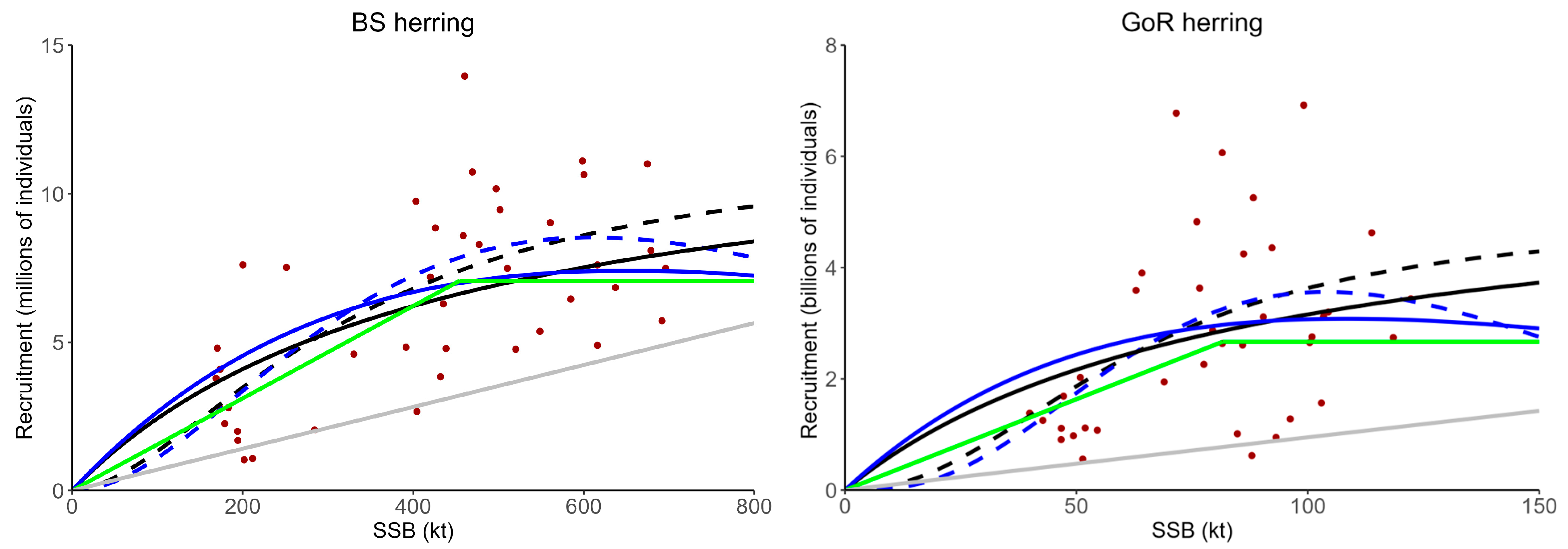
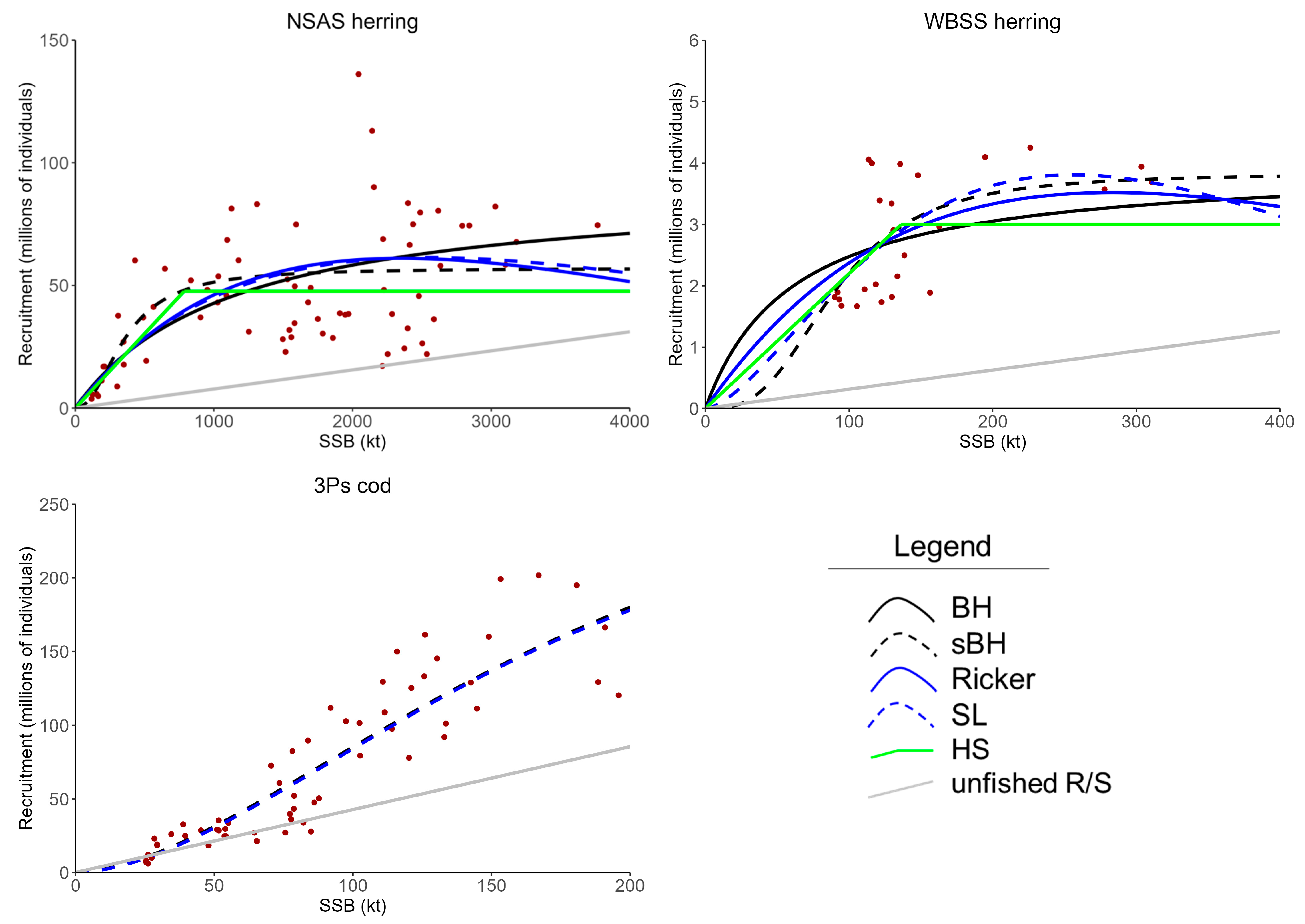
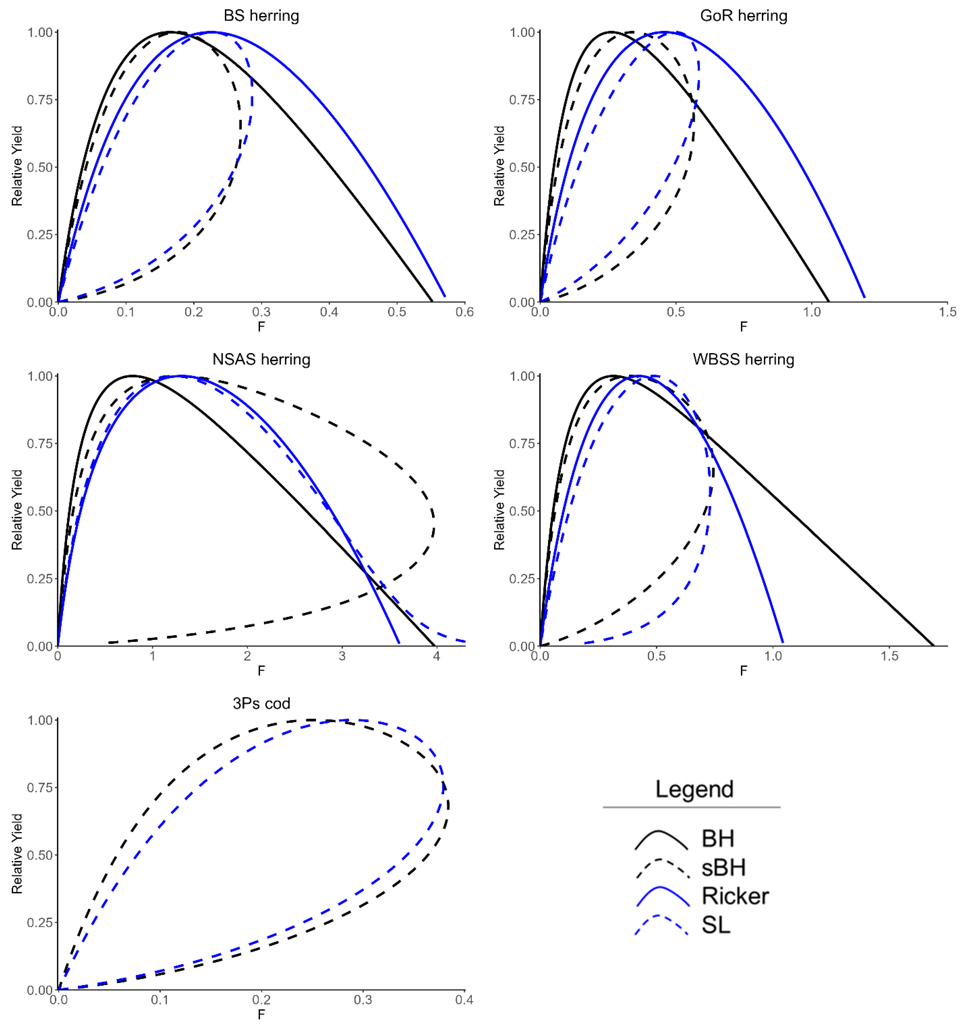
3.1. Model Fits and Comparison of Candidate LRPs

The five stock–recruit models were fit for each stock (Figure 1, Table S1, uncertainty in sBH and SL models shown in Figure S1) with the exception of 3Ps cod, for which the BH, Ricker, and HS models did not fit the data, which is clear from the pattern of the stock–recruit data in Figure 1. The depensation models were the best fit for each herring stock based on LOOIC, with the exception of the Ricker being better than SL for NSAS herring (Table S2). The sBH model was a better fit than SL for all herring stocks except GoR herring (Table S2). The posterior probabilities of $c$ > 1 (i.e., evidence of depensation) were greater than 0.8 for the sBH and SL models for all stocks, with the exception of the SL model for NSAS herring (Table S1; similar results previously reported in [21,22] and consistent with the model selection based on LOOIC). A ‘strong’ Allee effect (i.e., B_AT > 0; [13]) was detected for all sBH and SL models with the exception of the sBH model for NSAS herring and the SL model for WBSS herring (Table 1). The maximum depletion (B_AT/B₀) of the B_AT estimates was 0.10 for the SL model for GoR herring (Table 1). B_AET estimates occurred at a depletion (B_AET/B₀) of 0.053 to 0.21 for the BH and sBH models and 0.15 to 0.39 for the Ricker and SL models (Table 1 and Table 2; note that the B_AET estimates from the sBH and SL models were used to compare to 0.2 B₀ for the BH and Ricker models, respectively, in Table 2). This difference in depletion between models is more strongly influenced by differences in the magnitude of B₀ rather than in the magnitude of B_AET. The B_AET estimates from the sBH and SL models were similar in magnitude (within 17% relative difference; Table 1, Figure S2). The B_AET estimates from the sBH model exceeded 0.4 B_MSY for BS herring, GoR herring, and 3Ps cod (Table 1). For these three stocks, the B_AET estimates from the SL model also exceeded the traditional LRPs of 0.2 B₀ and 0.4 B_MSY (Table 1). The B_AET estimates from the sBH and SL models were also compared to B₀ and B_MSY estimates from the BH and Ricker models, respectively (Table 2). The addition of the depensation parameter did not have a strong influence on the level of depletion of the B_AET estimates but had some influence on the ratio of B_AET to B_MSY, where B_AET reached as high as 0.8 B_MSY for the Ricker model for GoR herring (Table 1 and Table 2). The B_AET estimates from the sBH and SL models ranged from 0.49 to 0.89 B_CP for each of the case study stocks (Table 1, Figure S2).

The SRRs with overcompensation at high biomass (i.e., Ricker and SL) result in much lower estimates of B₀ and B_MSY compared to the SRRs with asymptotic recruitment (i.e., BH and sBH) (Table 1, Figure S2). The overcompensation assumption (i.e., choosing Ricker over BH or choosing SL over sBH) results in a B_MSY estimate at a higher depletion level (Figure S3).

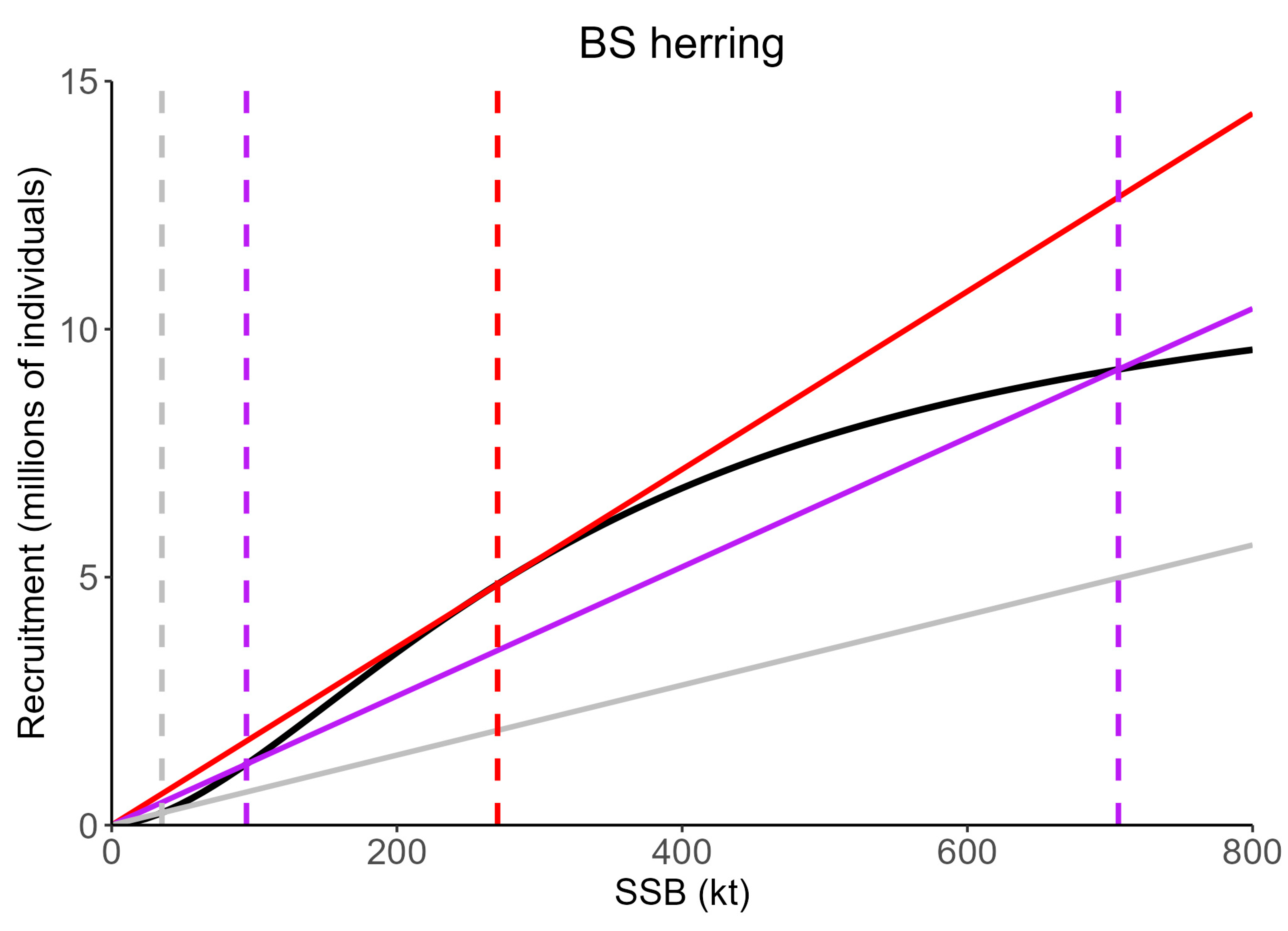
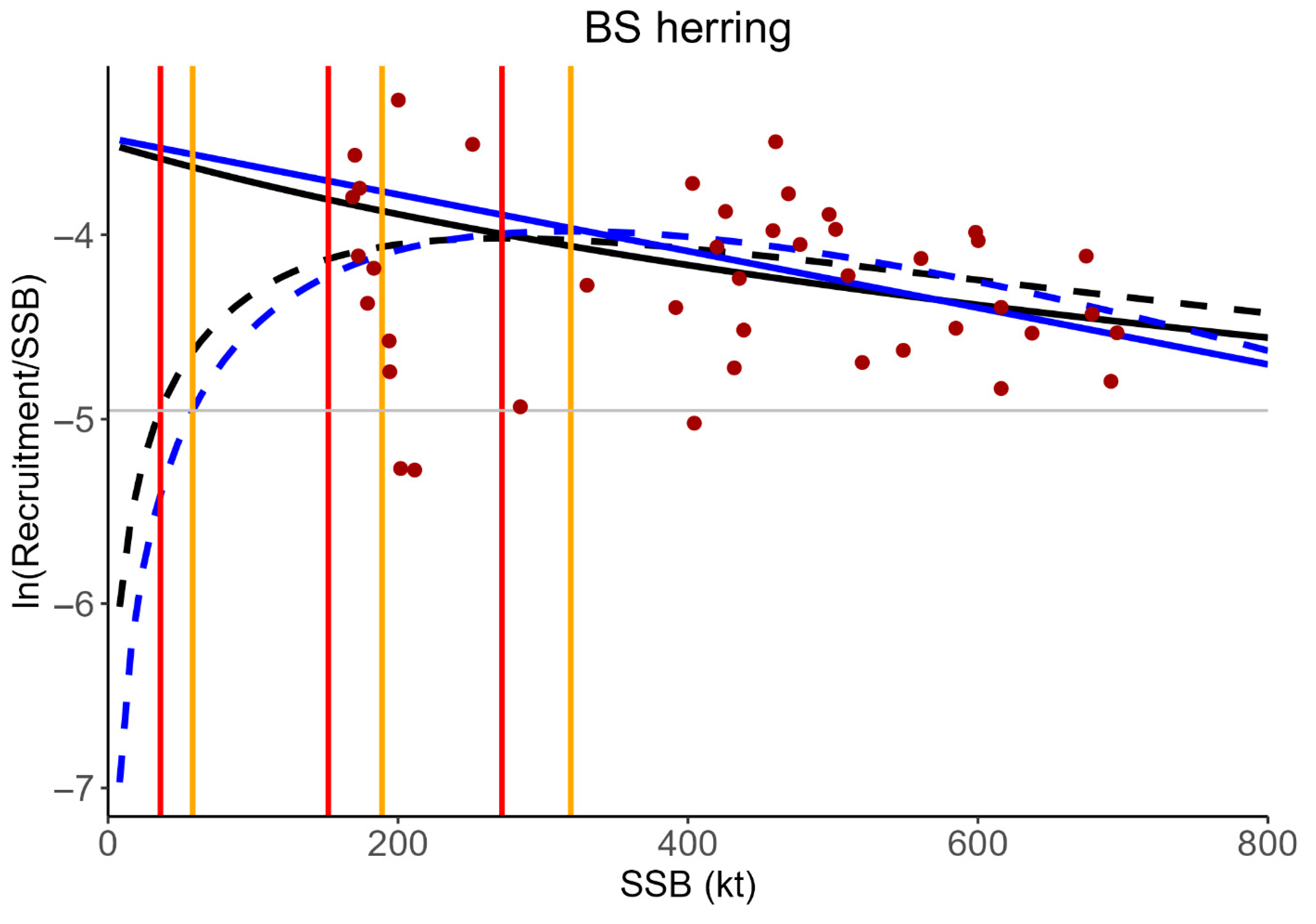
3.2. Stock Dynamics with Multiple Equilibrium States and F Reference Points

The potential for an inflection point in the depensatory models can lead to multiple intersection points of the SRR and the replacement line at a given F (Figure 2), implying multiple equilibrium states from fishing at a constant long-term F. This is illustrated in Figure 4 where the relative yield vs. F curves resemble a flower petal, with two solutions at the same F where the replacement line intersects the SRR (Figure 2). The interpretation of these curves is further supplemented by plotting SSB vs. F with the corresponding yield (Figure S4). When there are multiple intersections, the equilibrium yield and SSB depend on the initial biomass. If there is excess recruitment (i.e., the predicted recruitment is above the replacement line) at the initial biomass, then the stock will approach the upper equilibrium value. If there is no excess recruitment (i.e., predicted recruitment below the replacement line) at the initial biomass, then the stock will approach the lower equilibrium value, keeping in mind that the origin is another intersection point. For example, for F = 0.15 in Figure 2 and Figure S4, if the initial biomass is between 94.5 and 706 kt, the equilibrium SSB from fishing at F = 0.15 is 706 kt. If the initial projection biomass is less than 94.5 kt then the equilibrium SSB is 0 kt (lower intersection point), and if the initial biomass is greater than 706 kt then the equilibrium SSB is 706 kt.

Inclusion of the depensation term in the SRR had a significant influence on F_crash (i.e., the maximum F in Figure 4). For BS, GoR, and WBSS herring, F_crash is much lower for the sBH and SL models compared to the BH and Ricker models, and in some cases, not much greater than F_MSY in the non-depensatory models (Table 1, Figure 4). The convex shape of the SRR at low biomass in the sBH and SL models can have a large influence on the relative yield at low biomass. The difference in yield can be less than a third at the same level of depletion for the SL compared to the Ricker model (e.g., GoF herring at 0.2 depletion; Figure S3) and the relative yield can reach zero before the origin. The latter occurs when biomass falls below B_AT (e.g., yield is zero when biomass is below B_AT or 0.10 depletion for GoF herring with the SL model; Figure S3, Table 1). The only model with a depensation parameter $\mathit{c}$ that was estimated below 1 with probability > 0.5 (i.e., evidence to support compensation at all stock sizes) was the SL model for NSAS herring, and the relative yield vs. F curve had a tail at higher F (Figure 4), resulting in a greater F_crash than the Ricker model (Table 1).

4. Discussion and Conclusions

To our knowledge, an LRP (or equivalent threshold for fisheries management) has not been formally adopted for management of a stock based on an Allee effect threshold or depensation threshold estimated from an SRR, even though it is a stock state to be avoided and consistent with the intent of an LRP (e.g., avoid serious harm to the productivity of the stock [1]; avoid recruitment overfishing [9]). This is most likely related to the challenges in detecting depensation in SRRs. The ability to detect depensation in an SRR requires data at low biomass and/or requires passing the depensation threshold. Hilborn et al. [18] suggested that thresholds for depensation are well below commonly adopted LRPs. Allee effect thresholds have been estimated for a limited number of marine fishes in the range of 10–12% of the maximum observed abundance (N_max; [13]), and this threshold is consistent with an impaired-recovery threshold near 10% N_max supported by a meta-analysis of 153 stocks [49]. If an assumption is made that abundance is proportional to biomass and that the N_max is a proxy for B₀, then thresholds of 10–12% N_max would be generally less than traditional policy default reference points commonly applied in some jurisdictions (e.g., 0.4 B_MSY [1]; 0.2 B₀ [4]), suggesting that commonly used LRPs from compensatory SRRs are sufficient to guard against Allee effects. However, the estimates of B_AET in the present study indicated that Allee effect thresholds can exceed these commonly adopted LRPs based on B₀ and B_MSY. The magnitude of the discrepancy depended on the SRR model assumption, where the B_AET estimates from the SL model occurred at a higher depletion and higher proportion of B_MSY compared to the sBH model. This difference between models was primarily influenced by the descending portion of the SRR at high biomass (i.e., the hypothesis of over-compensation) influencing B₀ and not the absolute magnitude of B_AET. These findings suggest that Allee effect thresholds can exceed traditional policy default reference points (e.g., 0.4 B_MSY [1]; 0.2 B₀ [4]); however, for all five case study stocks, B_CP (defined based on the definition of B_lim in ICES [2]) was a conservative LRP and exceeded B_AET. estimated from both the sBH and SL models.

In the present study, we used the definition of an Allee effect threshold (B_AET) that is consistent with [13]; namely, the biomass below which the realized per capita population growth rate declines with declining biomass. This differs from B_inflection, which was defined as an “Allee effect threshold” in [22] and lies approximately at the midpoint of the B_AT and B_AET (Table 1, e.g., Figure 3). Given that the per capita recruitment begins to decline below B_AET (here it is assumed that per capita recruitment is a proxy for per capita growth), we feel that this reference point is more appropriate as a candidate LRP than B_inflection because B_AET is the threshold to depensation. The definition of a demographic Allee effect from [13] is based on the per capita population growth rate. We have assumed in the present study that per capita recruitment is a proxy for per capita population growth. Recruitment is a population level process that contributes to the per capita population growth rate; however, components of individual fitness (e.g., adult survival) could be density dependent and compensate for the reduced recruitment at low biomass [49,50]. Even if this were to occur and a true demographic Allee effect was not manifested at low biomass, depensation in the SRR is still consistent with the objectives of an LRP.

A common approach to selecting statistical models in fisheries science is to identify models with a parsimonious representation of the data using methods such as likelihood ratio tests (e.g., [16]) or AIC (e.g., [18,51]) using models estimated based on maximum likelihood estimation. In the absence of data at low stock sizes (i.e., in the region of an Allee effect threshold), model selection methods may be insufficient to detect depensation. Model selection methods such as AIC apply a penalty to models with additional parameters, so models that account for depensation are at a disadvantage using this approach, especially since many stock–recruit data sets have limited data at low biomass. While model selection methods are useful statistical tools in fisheries science and were able to identify models with depensation as the best model in each of the herring stocks in the present study, capturing uncertainty in stock dynamics at low biomass and considering the biology of the stock are important when selecting biologically plausible models. Two-parameter SRRs such as the traditional BH and Ricker models also restrict the range of B_MSY/B₀ [36] which is determined by the productivity of the stock (e.g., steepness of the SRR). An additional potential advantage of a three-parameter SRR model, in addition to the possibility to account for depensation, is that of no assumed implicit relationship between B₀ and B_MSY [36].

The SRRs explored in the present study assumed a positive relationship between recruitment and SSB with time-invariant SRR parameter estimates. Spurious SRRs can be deduced if recruitment is environmental driven or from a reversed causality of “boom and bust” dynamics for forage fishes such as herring, where changes in recruitment influence changes in SSB [52]. These potential concerns with fitting SRRs and the possibility of time-vary SRR parameters should be considered during the development of stock assessment models.

Liermann and Hilborn [14] suggest that challenges in detecting depensation in the SRR should not lead one to conclude that depensation is rare and/or unimportant. In the absence of data at low stock sizes, the potential for depensation becomes an uncertainty and ignoring this uncertainty can result in selecting management strategies that are not sufficiently robust [53]. For example, uncertainty in the form of the SRR could result in estimates of F_MSY from one model to be approximately F_crash in another model (see BS and GoR herring, Figure 4, Table 1). Management strategy evaluation [54,55] is one approach to deal with this uncertainty and a precautionary approach to providing scientific advice to management would be to evaluate whether harvest strategies are robust to the possibility of depensation [21]). If the difference between F_MSY and F_crash is smaller with depensatory SRRs than compensatory SRRs, then it will be more difficult to thread the needle of maintaining the target with high probability and avoiding the limit with even higher probability. If depensation exists, then management strategies will likely need to be either very responsive, more conservative with regard to long-term harvest rates, or both to reach management objectives.

The choice of SRR has significant implications for biological reference points and the perceived potential yield for the stock (Table 1, Figure S2). When defining LRPs, it can be useful to explore several candidate methods and look for agreements/disagreements among methods [56,57]. Agreement can provide confidence and flexibility in selecting an appropriate LRP while disagreement can identify potential risks (e.g., 0.4 B_MSY could occur below 0.1 B₀, indicating an extreme mismatch in biomass levels for defining serious harm due to high sensitivity to assumptions) [57]. For example, estimates of B_MSY depend strongly on the steepness of the SRR [58,59], and reliable estimation of steepness also depends on stock–recruit data at low biomass. Similarly, when there are few stock–recruit data points at high biomass, estimates of B₀ become more uncertain (e.g., see SRRs for GoR herring in Figure 1 for which B₀ estimates range from 187 to 520 kt; Table 1). LRPs in Canada are now being used in legislation to require a rebuilding plan under the Fish Stocks Provisions in the Fisheries Act [6], and selection of reference points will likely require greater scientific scrutiny than simply selecting the policy default [1]. Our comparison of candidate LRPs in the present study supports the recommendation to explore several candidate methods, including functional forms of the SRR and approaches/assumptions (e.g., proportions of B₀ vs. proportions of B_MSY vs. B_lim or B_CP) and showed that Allee effect thresholds may occur at a level higher than traditional LRPs defined by national policy defaults (e.g., 0.4 B_MSY in Canada and 0.2 B₀ in Australia) but below B_CP defined based on the ICES [2] guidance for setting B_lim.

The present study identifies an approach to define an LRP based on depensatory SRRs and describes population dynamics under depensation with equilibrium assumptions. Future work should focus on estimating the SRR parameters within the objective function of a stock assessment model to overcome the problems with using stock assessment estimates as independent observations in post hoc analyses [30,31]. While Allee effect thresholds may occur at a level higher than traditional LRPs defined by national policy defaults, future work should focus on evaluating the performance of the various candidate LRPs via simulation testing and the influence of time-varying productivity on projection dynamics in the presence of recruitment depensation. Given the difficulty in detecting depensation in SRRs, this structural uncertainty can be addressed with simulation testing of management strategies to identify strategies that are robust to depensatory effects.

References

1. DFO (Fisheries and Oceans Canada). A Fishery Decision-Making Framework Incorporating the Precautionary Approach. Last Updated 2009-03-23. 2009. Available online: https://www.dfo-mpo.gc.ca/reports-rapports/regs/sff-cpd/precaution-eng.htm (accessed on 20 May 2025).
2. ICES (International Council for the Exploration of the Sea). Technical Guidelines. In Report of the ICES Advisory Committee, 2021. ICES Advice 2021, Section 16.4.3.1. 2021. Available online: https://doi.org/10.17895/ices.advice.7891 (accessed on 20 May 2025).
3. eCFR (Electronic Code of Federal Regulations). Title 50: Wildlife and Fisheries, Part 600: Magnuson-Stevens Act Provisions, Subpart D: National Standards. 2021. Available online: https://www.ecfr.gov/cgi-bin/text-idx?SID=71b8c6026001cb90e4b0925328dce685&mc=true&node=se50.12.600_1310&rgn=div8 (accessed on 20 May 2025).
4. DAWR (Department of Agriculture and Water Resources, Australian Government). Guidelines for the Implementation of the Commonwealth Fisheries Harvest Strategy Policy. 2nd Edition. 2018. Available online: https://www.agriculture.gov.au/sites/default/files/sitecollectiondocuments/fisheries/domestic/hsp.pdf (accessed on 20 May 2025).
5. Sainsbury, K. Best Practice Reference Points for Australian Fisheries. Australian Fisheries Management Authority Report R2001/0999. 2008. Available online: https://www.agriculture.gov.au/sites/default/files/sitecollectiondocuments/fisheries/environment/bycatch/best-practice-references-keith-sainsbury.pdf (accessed on 20 May 2025).
6. DFO. Guidelines for Implementing the Fish Stocks Provisions in the Fisheries Act. Last Updated 2022-08-23. 2022. Available online: https://www.dfo-mpo.gc.ca/reports-rapports/regs/sff-cpd/guidelines-lignes-directrices-eng.htm (accessed on 20 May 2025).
7. MF (New Zealand Government, Ministry of Fisheries). Harvest Strategy Standard for New Zealand Fisheries. 2008. Available online: https://www.mpi.govt.nz/dmsdocument/728-Harvest-Strategy-Standard-for-New-Zealand-Fisheries (accessed on 20 May 2025).
8. Restrepo, V.R.; Thompson, G.G.; Mace, P.M.; Gabriel, W.L.; Low, L.L.; MacCall, A.D.; Methot, R.D.; Powers, J.E.; Taylor, B.L.; Wade, P.R.; et al. Technical Guidance on the Use of Precautionary Approaches to Implementing National Standard 1 of the Magnuson-Stevens Fishery Conservation and Management Act. NOAA Technical Memorandum NMFS–F/SPO–31. 1998. Available online: https://www.st.nmfs.noaa.gov/Assets/stock/documents/Tech-Guidelines.pdf (accessed on 20 May 2025).
9. Myers, R.A.; Rosenberg, A.A.; Mace, P.M.; Barrowman, N.; Restrepo, V.R. In search of thresholds for recruitment overfishing. ICES J. Mar. Sci. 1994, 51, 191–205. [Google Scholar] [CrossRef]
10. Hilborn, R.; Walters, C.J. Quantitative Fisheries Stock Assessment: Choice, Dynamics and Uncertainty; Chapman and Hall: New York, NY, USA, 1992; 570p. [Google Scholar]
11. Hutchings, J.A. Renaissance of a caveat: Allee effects in marine fish. ICES J. Mar. Sci. 2014, 71, 2152–2157. [Google Scholar] [CrossRef]
12. Allee, W.H. Animal Aggregations, A Study in General Sociology; University Chicago Press: Chicago, IL, USA, 1931. [Google Scholar]
13. Hutchings, J.A. Thresholds for impaired species recovery. Proc. R. Soc. Ser. B Biol. Sci. 2015, 282, 20150654. [Google Scholar] [CrossRef] [PubMed]
14. Liermann, M.; Hilborn, R. Depensation: Evidence, models and implications. Fish Fish. 2001, 2, 33–58. [Google Scholar] [CrossRef]
15. Kronlund, A.R.; Forrest, R.E.; Cleary, J.S.; Grinnell, M.H. The selection and role of limit reference points for Pacific herring (Clupea pallasii) in British Columbia, Canada. DFO Canadian Science Advisory Secretariat Research Document. 2018/009. 2018. ix + 125 p. Available online: https://waves-vagues.dfo-mpo.gc.ca/library-bibliotheque/40685147.pdf (accessed on 20 May 2025).
16. Myers, R.A.; Barrowman, N.J.; Hutchings, J.A.; Rosenberg, A.A. Population dynamics of exploited fish stocks at low population levels. Science 1995, 269, 1106–1108. [Google Scholar] [CrossRef]
17. Liermann, M.; Hilborn, R. Depensation in fish stocks: A hierarchic Bayesian meta-analysis. Can. J. Fish. Aquat. Sci. 1997, 54, 1976–1984. [Google Scholar] [CrossRef]
18. Hilborn, R.; Hively, D.J.; Jensen, O.P.; Branch, T.A. The dynamics of fish populations at low abundance and prospects for rebuilding and recovery. ICES J. Mar. Sci. 2014, 71, 2141–2151. [Google Scholar] [CrossRef]
19. Ricard, D.; Minto, D.; Jensen, O.P.; Baum, J.K. Examining the knowledge base and status of commercially exploited marine species with the RAM Legacy Stock Assessment Database. Fish Fish. 2012, 13, 380–398. [Google Scholar] [CrossRef]
20. Keith, D.M.; Hutchings, J.A. Population dynamics of marine fishes at low abundance. Can. J. Fish. Aquat. Sci. 2012, 69, 1150–1163. [Google Scholar] [CrossRef]
21. Perälä, T.; Kuparinen, A. Detection of Allee effects in marine fishes: Analytical biases generated by data availability and model selection. Proc. R. Soc. Ser. B Biol. Sci. 2017, 284, 20171284. [Google Scholar] [CrossRef]
22. Perälä, T.; Hutchings, J.A.; Kuparinen, A. Allee effects and the Allee-effect zone in northwest Atlantic cod. Biol. Lett. 2022, 18, 20210439. [Google Scholar] [CrossRef] [PubMed]
23. Marentette, J.R.; Kronlund, A.R.; Cogliati, K.M. Specification of precautionary approach reference points and harvest control rules in domestically managed and assessed key harvested stocks in Canada. DFO Canadian Science Advisory Secretariat Research Document. 2021/057. 2021. vii + 98 p. Available online: https://publications.gc.ca/collections/collection_2021/mpo-dfo/fs70-5/Fs70-5-2021-057-eng.pdf (accessed on 20 May 2025).
24. DFO. Stock Assessment of NAFO subdivision 3Ps cod. DFO Canadian Science Advisory Secretariat Science Advisory Report. 2020/018. Available online: https://publications.gc.ca/collections/collection_2020/mpo-dfo/fs70-6/Fs70-6-2020-018-eng.pdf (accessed on 20 May 2025).
25. ICES. Report of the Herring Assessment Working Group for the Area South of 62ºN (HAWG), 10–19 March 2015; ICES CM 2015/ACOM:06; ICES: Copenhagen, Denmark, 2015. [Google Scholar]
26. ICES. Report of the Baltic Fisheries Assessment Working Group (WGBFAS), 14–21 April 2015; ICES CM 2015/ACOM:10; ICES: Copenhagen, Denmark, 2015. [Google Scholar]
27. Varkey, D.A.; Babyn, J.; Regular, P.; Ings, D.W.; Kumar, R.; Rogers, B.; Champagnat, J.; Morgan, M.J. A state-space model for stock assessment of cod (Gadus morhua) stock in NAFO subdivision 3Ps. DFO Canadian Science Advisory Secretariat Research Document. 2022/022. 2022. v + 78 p. Available online: https://waves-vagues.dfo-mpo.gc.ca/library-bibliotheque/4105829x.pdf (accessed on 20 May 2025).
28. Neilson, A.; Berg, C.W. Estimation of time-varying selectivity in stock assessments using state-space models. Fish. Res. 2014, 158, 96–101. [Google Scholar] [CrossRef]
29. Shepherd, J.G. Extended survivors analysis: An improved method for the analysis of catch-at-age data and abundance indices. ICES J. Mar. Sci. 1999, 56, 584–591. [Google Scholar] [CrossRef]
30. Link, W.A. Modeling pattern in collections of parameters. J. Wildl. Manag. 1999, 63, 1017–1027. [Google Scholar] [CrossRef]
31. Brooks, E.N.; Deroba, J.J. When “data” are not data: The pitfalls of post hoc analyses that use stock assessment model output. Can. J. Fish. Aquat. Sci. 2015, 72, 634–641. [Google Scholar] [CrossRef]
32. Beverton, R.J.H.; Holt, S.J. On the Dynamics of Exploited Fish Populations; Ministry of Agriculture, Fisheries and Food. Fishery Investigations: London, UK, 1957; p. 533. [Google Scholar]
33. Ricker, W.E. Stock and recruitment. J. Fish. Res. Board Can. 1954, 11, 559–623. [Google Scholar] [CrossRef]
34. Saila, S.; Recksiek, C.W.; Prager, M.H. Basic Fishery Science Programs; Elsevier: Amsterdam, The Netherlands, 1988; 230p. [Google Scholar]
35. Iles, T.C. A review of stock-recruitment relationships with reference to flatfish populations. Neth. J. Sea Res. 1994, 32, 399–420. [Google Scholar] [CrossRef]
36. Punt, A.E.; Cope, J.M. Extending integrated stock assessment models to use non-depensatory three-parameter stock-recruitment relationships. Fish. Res. 2019, 217, 46–57. [Google Scholar] [CrossRef]
37. Miller, T.J.; Brooks, E.N. Steepness is a slippery slope. Fish Fish. 2020, 22, 634–645. [Google Scholar] [CrossRef]
38. Guo, J.; Gabry, J.; Goodrich, B.; Johnson, A.; Weber, S.; Badr, H.S.; Lee, D.; Sakrejda, K.; Martin, M.; Trustees of Columbia University; et al. R Interface to Stan. Package ‘rstan’, Version 2.32.7. 2025. Available online: https://cran.r-project.org/web/packages/rstan/rstan.pdf (accessed on 20 May 2025).
39. Gabry, J.; Veen, D.; Stan Development Team; Andreae, M.; Betancourt, M.; Carpenter, B.; Gao, Y.; Gelman, A.; Goodrich, B.; Lee, D.; et al. Interactive Visual and Numerical Diagnostics and Posterior Analysis for Bayesian Models. Package ‘shinystan’. Version 2.6.0. 2022. Available online: https://cran.r-project.org/web/packages/shinystan/shinystan.pdf (accessed on 20 May 2025).
40. Stan Development Team. Stan Reference Manual. 2025. Available online: https://mc-stan.org/ (accessed on 20 May 2025).
41. Vehtari, A.; Gelman, A.; Gabry, J. Practical Bayesian model evaluation using leave-one-out cross-validation and WAIC. Stat. Comput. 2017, 27, 1413–1432. [Google Scholar] [CrossRef]
42. Vehtari, A.; Gabry, J.; Magnusson, M.; Yao, Y.; Bürkner, P.-C.; Paananen, T.; Gelman, A.; Goodrich, B.; Piironen, J.; Nicenboim, B.; et al. Efficient Leave-One-out Cross-Validation and WAIC for Bayesian Models. Package ‘loo’. Version 2.8.0. 2024. Available online: https://cran.r-project.org/web/packages/loo/loo.pdf (accessed on 20 May 2025).
43. Akaike, H. A new look at the statistical model identification. IEEE Trans. Autom. Control. 1974, 19, 716–723. [Google Scholar] [CrossRef]
44. Maunder, M.N. Stock-recruitment models from the viewpoint of density-dependent survival and the onset of strong density-dependence when a carrying capacity limit is reached. Fish. Res. 2022, 249, 106249. [Google Scholar] [CrossRef]
45. Soetaert, K.; Hindmarch, A.C.; Eisenstat, S.C.; Moler, C.; Dongarra, J.; Saad, Y. Nonlinear Root Finding, Equilibrium and Steady-State Analysis of Ordinary Differential Equations. Package ‘rootSolve’. Version 1.8.2.3. 2022. Available online: https://cran.r-project.org/web/packages/rootSolve/rootSolve.pdf (accessed on 20 May 2025).
46. Brooks, E.N.; Powers, J.E. Generalized compensation in stock-recruit functions: Properties and implications for management. ICES J. Mar. Sci. 2007, 64, 413–424. [Google Scholar] [CrossRef]
47. Barrowman, N.J.; Myers, R.A. Still more spawner-recruitment curves: The hockey stick and its generalizations. Can. J. Fish. Aquat. Sci. 2000, 57, 665–676. [Google Scholar] [CrossRef]
48. R Core Team. R: A Language and Environment for Statistical Computing. R Foundation for Statistical Computing, Vienna, Austria. 2025. Available online: https://www.R-project.org/ (accessed on 20 May 2025).
49. Neubauer, P.; Jensen, O.P.; Hutchings, J.A.; Baum, J.K. Resilience and recovery of overexploited marine populations. Science 2013, 340, 347–349. [Google Scholar] [CrossRef]
50. Stephens, P.A.; Sutherland, W.J.; Freckleton, R.P. What is the Allee effect? Oikos 1999, 87, 185–190. [Google Scholar] [CrossRef]
51. Holt, C.A.; Michielsens, C.G.J. Impact of time-varying productivity on estimated stock–recruitment parameters and biological reference points. Can. J. Fish. Aquat. Sci. 2020, 77, 836–847. [Google Scholar] [CrossRef]
52. Szuwalski, C.S.; Britten, G.L.; Licandeo, R.; Amoroso, R.O.; Hilborn, R.; Walters, C. Global forage fish recruitment dynamics: A comparison of methods, time-variation, and reverse causality. Fish. Res. 2019, 214, 56–64. [Google Scholar] [CrossRef]
53. Punt, A.E. Refocusing stock assessment in support of policy evaluation. In Fisheries for Global Welfare and Environment, Proceedings of the 5th World Fisheries Congress 2008, Yokohama, Japan, 20–24 October 2008; Tsukamoto, K., Kawamura, T., Takeuchi, T., Beard, T.D., Kaiser, M.J., Eds.; TERRAPUB: Tokyo, Japan, 2008; pp. 139–152. [Google Scholar]
54. Butterworth, D.S.; Punt, A.E. Experiences in the evaluation and implementation of management procedures. ICES J. Mar. Sci. 1999, 56, 985–998. [Google Scholar] [CrossRef]
55. Punt, A.E.; Butterworth, D.S.; de Moor, C.L.; Oliveira, J.A.A.; Haddon, M. Management strategy evaluation: Best practices. Fish Fish. 2016, 17, 303–334. [Google Scholar] [CrossRef]
56. van Deurs, M.; Brooks, M.E.; Lindengren, M.; Henriksen, O.; Rindorf, A. Biomass limit reference points are sensitive to estimation method, time-series length and stock development. Fish Fish. 2021, 22, 18–30. [Google Scholar] [CrossRef]
57. ICES. Workshop on ICES Reference Points (WKREF1). ICES Scientific Reports. 2022, Volume 4, Issue 2, 70p. Available online: http://doi.org/10.17895/ices.pub.9822 (accessed on 20 May 2025).
58. Haltuch, M.A.; Punt, A.E.; Dorn, M.W. Evaluating alternative estimators of fishery management reference points. Fish. Res. 2008, 94, 290–303. [Google Scholar] [CrossRef]
59. Punt, A.E.; Dorn, M.W.; Haltuch, M.A. Evaluation of threshold management strategies for groundfish off the U.S. West Coast. Fish. Res. 2008, 94, 251–266. [Google Scholar] [CrossRef]
Figure 1. Stock–recruit pairs and estimated stock–recruitment relationships based on the Beverton–Holt (BH), sigmoid BH (sBH), Ricker, Saila–Lorda (SL), and hockey stick (HS) models. The BH, Ricker, and HS models did not fit the data for 3Ps cod. The gray line represents the unfished replacement (R/S) line.
Fishes 10 00342 g001aFishes 10 00342 g001b
Figure 2. The sigmoid Beverton–Holt model for BS herring (black line) with the equilibrium unfished replacement line (gray line) intersecting the stock–recruitment relationship (SRR) at BAT (vertical dashed gray line), a replacement line for Fcrash (red line),the tangent to the SRR at BAET (vertical dashed red line), and a replacement line for F = 0.15 (purple line) intersecting the SRR at two points (the thresholds for excess recruitment at F = 0.15; vertical dashed purple lines).
Fishes 10 00342 g002
Figure 3. Plot of ln(Recruitment/SSB) vs. SSB (points) for BS herring and model fits for the Beverton–Holt (BH; black), sigmoid BH (sBH; dashed black), Ricker (blue), and Saila–Lorda (SL; dashed blue) models. The horizontal gray line is the unfished ln(Recruitment/SSB) and intersects the sBH and SL curves at BAT. The maximum ln(Recruitment/SSB) occurs at BAET. Vertical lines are BAT < Binflection < BAET, for the sBH model (red) and the SL model (orange).
Fishes 10 00342 g003
Figure 4. Relative yield vs. fishing mortality rate (F) by stock and stock–recruitment relationship. The BH and Ricker models did not fit the 3Ps cod data.
Fishes 10 00342 g004