Study on the Flow Velocity Preference of the Four Major Chinese Carps Using Convolutional Neural Networks

Abstract

Flow velocity is a critical factor in determining the suitability of fish habitats. Understanding the preference patterns of the four major Chinese carps (FMCCs) for different flow velocities is crucial for their habitat conservation and restoration. In this study, the preference of individual fish species, approximately 15 cm in length, for flow velocity was investigated at flow velocity gradients of 0.0, 0.4, 0.8, 1.2, 1.6, and 2.0 times their body length. Additionally, a deep learning algorithm based on convolutional neural networks (CNNs) was employed for fish target detection. The results showed that, at this length, black carp (Mylopharyngodon piceus) preferred fast currents when the inlet flow velocity was between 0.4 and 1.6 times their body length, while grass carp (Ctenopharyngodon idella), silver carp (Hypophthalmichthys molitrix), and bighead carp (Hypophthalmichthys nobilis) preferred fast currents when the inlet flow velocity of the test flume was between 0.4 and 2.0 times their body length. However, this preference for fast currents decreased as the overall flow velocity increased to a specific threshold, eventually leading to their avoidance. The highest preference for fast currents among the four species was observed at inlet flow velocities of 1.2, 0.4, 0.8, and 0.8 times their body length, respectively. The findings of this study provide important insights into habitat conservation and restoration for the FMCCs in projects focused on the construction of navigation channels and water conservancy.

1. Introduction

Flow velocity and flow patterns within the aquatic living environment are decisive for the survival and growth of fish. Variations in fish morphology are significantly influenced by the flow velocity in their habitats, with fish body shapes similarly responding to flow velocity across diverse watersheds [1]. Fluctuations in water flow velocity significantly affect not only fish behavioral patterns, such as tail flicking and schooling [2], but also their feeding behavior [3], growth [4], material metabolism [5], muscle quality [6], and even survival and reproduction [7,8]. Consequently, flow velocity and flow patterns are considered crucial determinants of the suitability of fish habitats.

The four major Chinese carps (FMCCs)—black carp (Mylopharyngodon piceus), grass carp (Ctenopharyngodon idella), silver carp (Hypophthalmichthys molitrix), and bighead carp (Hypophthalmichthys nobilis)—are significant economic fish species in China [9]. The ecological habits of these species and the impacts of water engineering projects on them [9,10], as well as methods for the conservation and restoration of their habitats [11], have been popular topics in fish ecology research in China. Determining the optimal and preferred flow velocities of the FMCCs can offer crucial data and theoretical support for the conservation and restoration of their wild habitats. Previous studies have explored the flow velocity preferences of FMCCs at the larval stage [7]. However, in-depth comparative studies involving laboratory-controlled experiments at different life history stages can contribute to a better understanding of their preference patterns and adaptation strategies regarding flow velocity during these distinct periods.

With the development of numerous deep learning models such as Image Net [12], VGGNet (Visual Geometry Group Net) [13], Residual Net [14], Dense Net [15], and Mobile Net [16], deep learning-based object detection methods have been widely applied for image classification. Some researchers have employed convolutional neural network models for the object detection of aquatic organisms such as fish and have achieved some results [17,18]. However, most of these studies are limited to the automatic identification of fish species in natural or aquaculture waters, and few attempts have involved the application of these models for fish location identification in behavioral experiments. Deep learning models detect objects by learning their features using a large volume of training data and extracting them from images with noisy and complex backgrounds. Moreover, their detection accuracy is less affected by environmental changes than commonly used image threshold segmentation methods in fish behavior research, and they have relatively high efficiency and accuracy [19]. Therefore, in fish ethology research, the application of deep learning-based image classification and object detection technologies to the detection and location identification of experimental fish could significantly improve the efficiency and accuracy of behavioral data analysis.

In this study, we introduced a deep learning object detection algorithm based on convolutional neural networks (CNNs) to investigate the preference behavior of FMCCs (with a body length of approximately 15 cm) across different flow velocities. This research not only provides a reference for optimal flow velocities in the artificial breeding of the four major Chinese carps but also offers theoretical insights for the restoration and reconstruction of their habitats in water engineering projects.

2. Materials and Methods

2.1. Animals and Housing

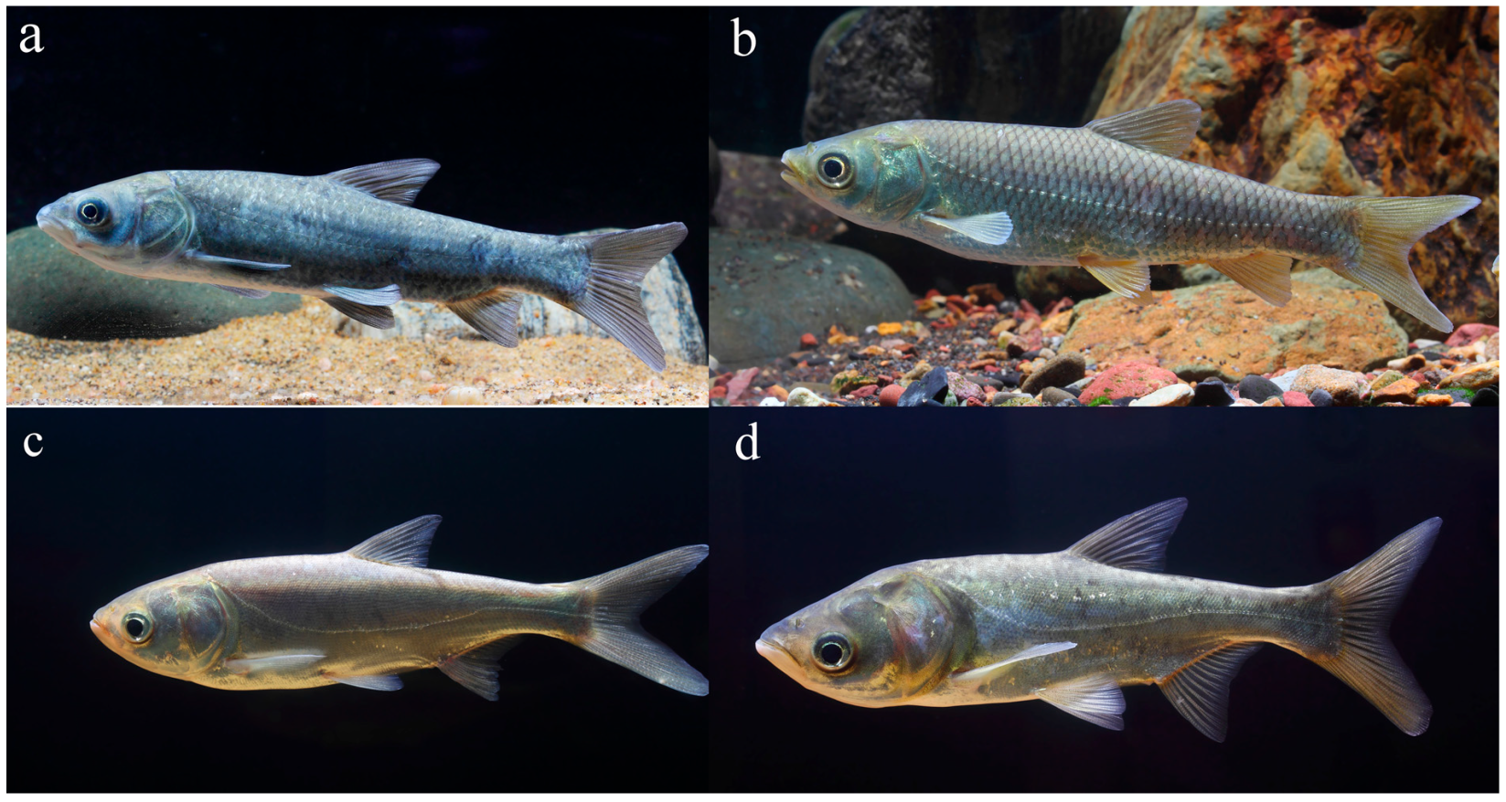
For this study, black carp (body length: 14.90 ± 0.36 cm), grass carp (body length: 15.13 ± 0.40 cm), silver carp (body length: 15.02 ± 0.39 cm), and bighead carp (body length: 15.09 ± 0.40 cm) were sourced from, Yuzhenduo Aquaculture Co., Ltd., Meishan, China. The appearance of four kinds of fish was shown in Figure 1. The experimental fish were reared in a recirculating aquaculture system similar to the experimental environment. During the experiment, from 08:00 to 22:00 every day, this aquaculture system was illuminated using fluorescent tubes placed at the top, with 80–100 lux of light intensity. Water temperature, pH, and dissolved oxygen were monitored daily (with an HQ30d device; Hach, Loveland, CO, USA) and maintained at 25 to 27 °C, 7.32 to 8.75, and 7.22 to 8.54 mg/L, respectively. All fish were fed to satiation twice daily with ozone-disinfected frozen red worms (Chironomidae flaviplumus larva; Yuerle, Tianjin, China).

2.2. Test Procedures and Apparatus

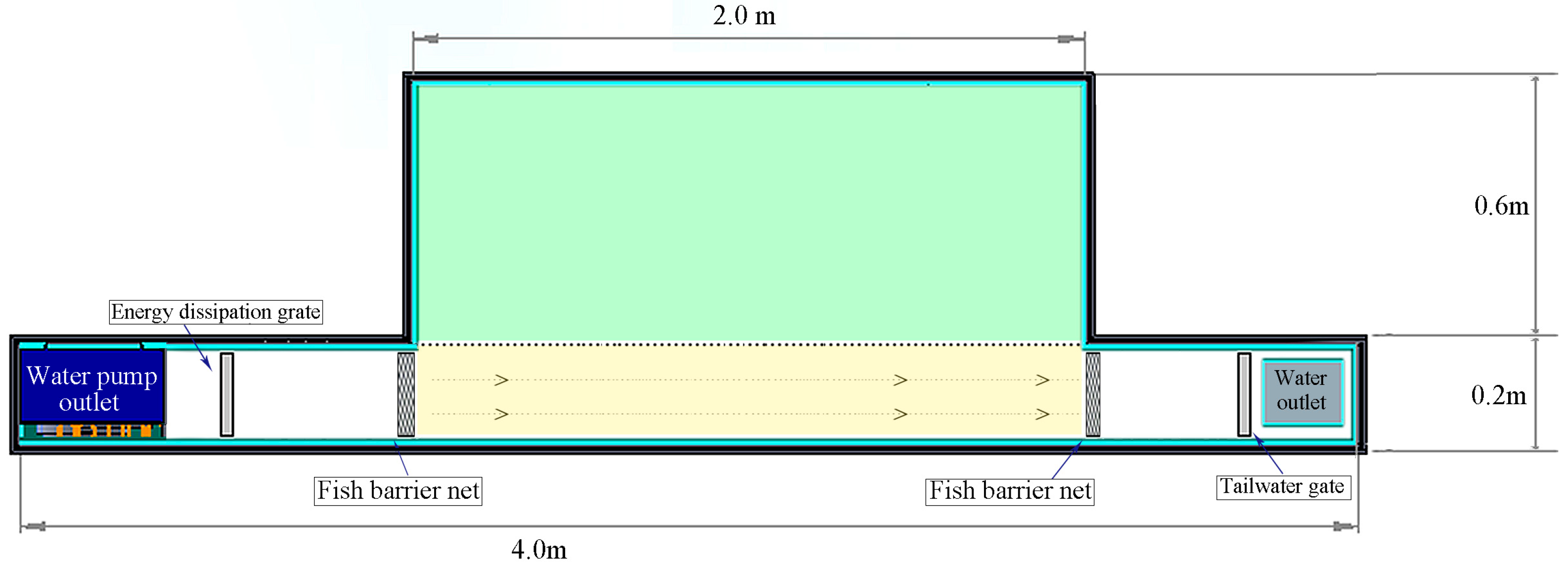
The experimental apparatus consisted of a T-shaped flume with a unilateral sudden expansion, the main body of which was 4.0 m in length, 0.8 m in width, and 0.6 m in height (Figure 2). The lower part of the flume featured a reservoir for water storage. In the experiments, water was pumped from the reservoir at the front of the flume, passing through a grate for energy dissipation and rectification, and entering the test section of the flume. Then, it flew through a straight channel into the rear part of the flume and returned to the reservoir via a drainage outlet. A tailgate was installed in front of the drainage outlet to control the water depth within the flume. When water passed through the test section, a rapid flow area (2.0 m in length and 0.2 m in width) was formed in the straight channel, while a slow flow area was formed in the adjacent space with dimensions of 2.0 m in length and 0.6 m in width, resulting in the spatial differentiation of flow velocities. Fish nets were installed at both the front and rear of the test section to prevent the experimental fish from leaving the test area. A high-definition CCD camera with a field of view covering the entire test section was installed at the top of the test section of the flume.

The experiment was conducted with five inlet flow velocity gradients for each fish species (i.e., the flow velocities when the water entered the test section). These gradients were set at 0, 0.4, 0.8, 1.2, 1.6, and 2.0 times the average body length (BL) of the experimental fish (0.15 m), corresponding to velocities of 0.06 m/s, 0.12 m/s, 0.18 m/s, 0.24 m/s, and 0.30 m/s, respectively. For each velocity tested, the flow velocities of the rapid and slow flow areas were measured by the multi-point velocity measurement method before the experiments started. Specifically, the rapid flow area and slow flow area were all divided into several 10 cm×10 cm grids, and a flow velocity meter (LS1206B, BAIFENG, Qingdao, China) was used to measure the velocity at the center point of each grid. For the center point of each grid, the flow velocity of the upper part (0.05 m below the water surface), the middle part (0.25 m below the water surface), and the bottom part of the water layer were measured. The measurement probe stayed in the water for 30 s during each measurement, and the value of flow velocity was recorded after the numerical display of the instrument stabilized. The flow velocity of each grid was defined as the average of the surface flow velocity, the middle flow velocity, and the bottom flow velocity at the central point of this grid. The flow velocity of the rapid flow area was determined as the average of the flow velocities of all the grids it contains, and the flow velocity of the slow flow area was calculated in the same way. The flow velocities in each area of different experimental groups were shown in

Table 1. Average flow velocities at various locations within the experimental area.

Groups	Inlet Flow Velocity (m/s)	Rapid Flow Area (m/s)	Slow Flow Area (m/s)
0 BL	0.000	0.000 ± 0.000	0.000 ± 0.000
0.4 BL	0.062	0.051 ± 0.006	0.012 ± 0.005
0.8 BL	0.123	0.100 ± 0.022	0.023 ± 0.005
1.2 BL	0.178	0.133 ± 0.023	0.042 ± 0.013
1.6 BL	0.239	0.193 ± 0.017	0.051 ± 0.016
2.0 BL	0.301	0.227 ± 0.031	0.076 ± 0.023

.

The flume was filled with water before the experiment, and the water depth was controlled at 0.5 m using the tailgate. Then, the water pump was stopped to allow the water in the flume to reach a static state. In each experiment, a single fish was carefully moved to the test section and allowed to freely swim within it. After a 10 min adaptation period, the CCD camera at the top of the flume began to continuously record the behavior of the experimental fish for 5 min when the water was still. Subsequently, the water pump was turned on, and its operating power was adjusted according to the velocity gradient settings. The inlet flow velocity was gradually increased in increments, and fish behavior was recorded for 5 min at each velocity until reaching the maximum velocity in the experiment. Then, the water pump was turned off, and the experimental fish were removed from the flume. Five specimens of each species were individually tested (five replicates), and no fish were reused. The fish behavior data were stored in mp4 video file format.

2.3. Detection of the Positions of Fish

2.3.1. Training of the Deep Learning Model

A total of 800 representative images were extracted from the recorded behavior videos. The extracted representative images encompassed the behavior states of the FMCCs at various flow velocities and were used to create the dataset required for model training. The experimental fish in the representative frames were labeled using labelimg 2.0 to generate corresponding label information for each image. The 800 data labels were divided into training and validation sets in a 7:1 ratio, with the training set comprising 700 data labels and the validation set containing 100 data labels. Then, transfer training was carried out on the dataset using the pretrained YOLOv5.pt weight file and the YOLOv5s model. The training results indicate that the mean average precision (mAP, an important metric for evaluating model performance) reached 0.95, and the target prediction results in the validation set were consistent with the manual annotation information in the training set. After training, the weight file used for individual fish detection was obtained.

2.3.2. Testing of the Deep Learning Model

Six images were randomly selected from the behavior videos of each fish species at each velocity group, resulting in a test set comprising 120 images, which was used to assess the performance of the above-trained YOLOv5 model in detecting individual fish in this study. The detection results of part of the test set are shown in Figure 3. It can be observed that the mean average precision (mAP) values for the detection of the four species were all around 0.9. The contours of the experimental fish can be clearly distinguished from the experimental background, and the visual effects are within an acceptable range for human eyes. No false detections or misdetections occurred, highlighting the superior performance of the proposed model for the identification of individual fish.

2.3.3. Detection of the Positions of Fish Using the Deep Learning Model

The weight file generated by the deep learning model was employed to perform object detection on all video data obtained in this study. The position information of the detected experimental fish targets in each frame was acquired and stored. Figure 4 shows the fish-identification process of the YOLOv5 model using the behavior videos. First, the above-mentioned trained weight file was loaded into the model, and then the recorded behavior video was read frame by frame and translated into images, which were used as input. Then, slicing was carried out using the Focus module to initially transform the feature size, converting the original images to 640 × 480 samples, which were more convenient for the model to operate. The transformed images were inputted into the backbone network composed of multiple convolutional layers, C3 modules, etc. and object features were extracted layer by layer. Then, in the neck network, using convolution and concat, the features at different scales were combined to enhance feature representation. Finally, the head detection network was used for the classification and identification of the experimental fish in the images at multiple scales, outputting the detection results using the position data of each fish species.

2.4. Data Analysis

According to the position coordinates of the experimental fish, the number of entries per square centimeter into each area during the experiment was counted. All data were analyzed for normal distribution and homogeneity of variance using the Kolmogorov–Smirnov and Levene methods, respectively. An independent-samples t-test was employed to analyze the differences in the total frequency of entries into the rapid and slow flow areas for the four species within each experimental group. Additionally, based on the total frequency data of experimental fish entering the rapid flow area across different flow velocity groups, inter-group differences in rheotaxis behavior were analyzed using the LSD (least significant difference) and Tamhane’s T2 multiple comparison methods.

3. Results

Figure 5a displays the number of black carp per square centimeter in rapid and slow flow areas across different velocities. No significant differences were found between entries into rapid and slow flow areas under static water (0.0 BL) or at an inlet velocity of 2.0 BL (p > 0.05), indicating no directional preference. Occupancy in the rapid flow area was significantly higher than that in the slow flow area when inlet velocities were 0.4 BL, 0.8 BL, 1.2 BL, and 1.6 BL (p < 0.05), demonstrating positive rheotaxis. The rheotaxis response progressively decreased as velocity increased beyond 1.2 BL, ultimately resulting in the avoidance of the rapid flow area at the maximum velocity (2.0 BL).

Figure 5b demonstrates grass carp’s distribution patterns. No zonal preference was detected under static water (p = 0.144). When the inlet flow velocity increased to 0.4 BL, the number of grass carp entering the rapid flow area was significantly higher than that in the slow flow area (p < 0.001). However, after the inlet flow velocity increased to 0.4 BL, the number of grass carp entering the rapid flow area gradually decreased with the increase in flow velocity, and they exhibited no obvious preference for either of the two areas at the highest flow velocity of 2.0 BL (p > 0.05).

Figure 5c reveals the behavioral responses of silver carp. No significant differences were observed in the number of silver carp entering the two areas (p = 0.150) in static water. When the inlet flow velocity increased to 0.4 BL, the number of fish entering the rapid flow area was significantly higher than that in the slow flow area (p < 0.001), and the fish consistently preferred the rapid flow area as the inlet flow velocity gradually increased; that is, the number of silver carp entering the rapid flow area was always higher than that in the slow flow area (p < 0.05). Nevertheless, when the inlet flow velocity increased to 2.0 BL, the preference of silver carp for the rapid flow area began to exhibit a downward trend.

Figure 5d shows the number of bighead carp per square centimeter in the rapid and slow flow areas at each velocity. All six velocities were associated with significantly higher rapid flow entries (p < 0.05). Notably, the number of bighead carp entering the rapid flow area began to decrease with the increase in flow velocity after the inlet flow velocity reached 1.2 BL.

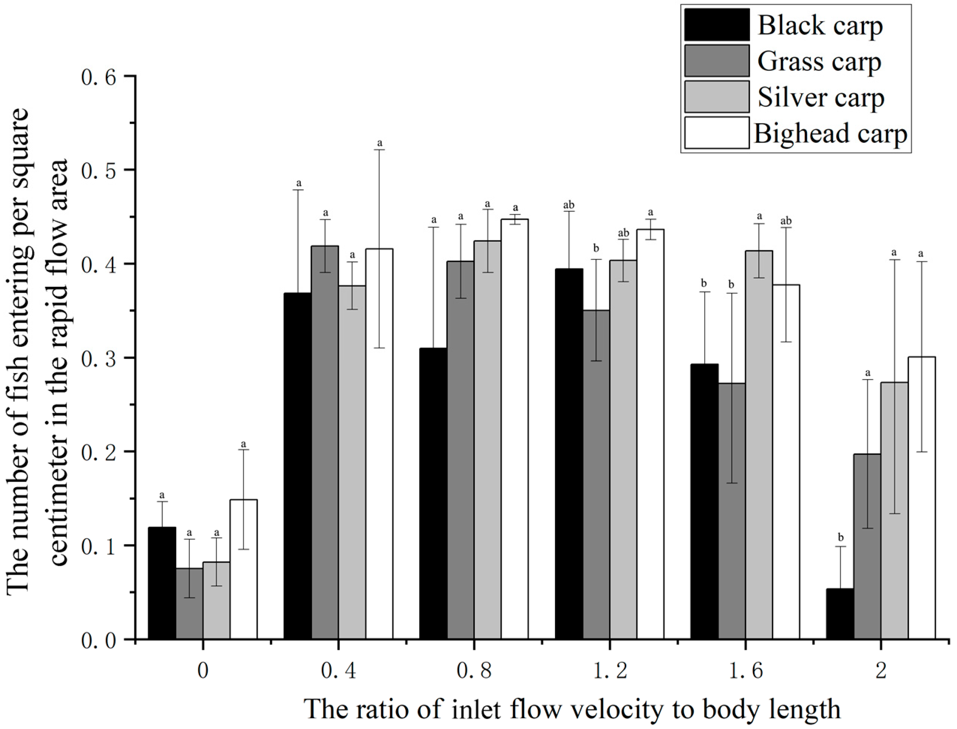
Figure 6 illustrates the fish distribution in the rapid flow area as an indicator of the degree of rheotaxis, which was used for interspecies comparison. At inlet flow velocities of 0 BL, 0.4 BL, and 0.8 BL, no obvious differences were observed in the distribution of the four fish species in the rapid flow area (p > 0.05). When the inlet flow velocity was 1.2 BL, the number of grass carp entering the rapid flow area was significantly lower than that of bighead carp (p = 0.014). At an inlet flow velocity of 1.6 BL, the total frequency of black carp and grass carp entering the rapid flow area was significantly lower than that of silver carp (p < 0.05). At an inlet flow velocity of 2.0 BL, the number of grass carp entering the rapid flow area was significantly lower than that of black carp (p = 0.048), silver carp (p = 0.038), and bighead carp (p = 0.027).

4. Discussion

According to the experimental results, the four fish species—grass carp, black carp, silver carp, and bighead carp—all exhibited significant rheotaxis. Variations in flow velocity in the environment lead to their preference for faster-flowing waters. Specific differences were observed in the rheotactic behavioral patterns among the four fish species. Overall, their behavioral patterns were relatively similar at low flow velocities below 1.6 body length (BL), but at high flow velocities above 1.6 BL, the rheotaxis of black carp and grass carp was relatively less than that of silver carp and bighead carp. All four fish species preferred rapid flow areas when the overall flow velocity was low but avoided them when the overall flow velocity was high. They exhibited the strongest avoidance of rapid flow areas when the inlet flow velocity was approximately 2.0 BL, with this pattern more evident in black carp and grass carp than in silver carp and bighead carp. The different flow velocity preferences directly affect the efficiency of food acquisition among these four major Chinese carp species. For instance, appropriate flow velocities can facilitate feeding and enhance foraging efficiency, with plankton directly flowing into the mouths of filter-feeding fish when they open their mouths against the current. For herbivorous fish such as grass carp, flowing water may bring aquatic plants to areas where they are more easily accessible. Omnivorous fish may search for various food resources in different flow velocity zones, with relatively flexible flow velocity preferences to adapt to different food source distributions.

Furthermore, compared to black carp and grass carp, silver carp and bighead carp prefer to swim more frequently in still water, resulting in more diverse and dispersed behavioral trajectories. Based on the research team’s observations of swimming behavior among various freshwater fish in China, compared to bottom-dwelling fish such as Gobioninae, Cyprinus sp. and Cobitidae, surface-dwelling fish such as Hemiculter leucisculus, Culter sp. and Hyporhamphus sp. markedly prefer to swim more frequently. Additionally, the swimming frequency of silver carp and bighead carp may also be related to their feeding habits. Silver carp and bighead carp are filter-feeding fish and thus need to constantly swim in natural waters to better filter out plankton in the water. Previous studies have reported that, among the four major Chinese carp species, silver carp and bighead carp exhibit flow velocity preferences that are closely associated with their feeding habits [20]. However, it has been established that filter-feeding fish have a significantly greater preference for still or slow-moving water than omnivorous and herbivorous fish, which relatively differs from our findings, potentially due to differences in experimental environments and methods. In addition, bighead carp individuals consistently showed a preference for staying upstream near the inlet against the current throughout the experiment. The authors currently cannot provide a reasonable explanation for the specific mechanism of this behavior, and the team will continue to investigate this issue.

In this study, we observed one fish at a time when studying the rheotactic behavior of the four major Chinese carp species. Significant individual behavioral differences were observed among the four fish species, resulting in high standard deviations in experimental data when using individual fish for research. The four major Chinese carp species are schooling fish in both natural and artificial breeding environments, and therefore, due to the presence of the “leader fish effect”, behavioral differences among individuals within schools may be masked, resulting in a more consistent behavioral pattern. Studies have shown that when schooling fish are isolated, they may exhibit abnormal and stereotypical behaviors [21]. We estimate that if fish schools were used in this study, the results might differ from those based on individual fish. Therefore, our research team plans to conduct similar rheotactic behavior studies using schools of the four major Chinese carp species to further explore the mechanisms of their rheotactic behavior.

Apart from rheotactic behavior, the results of this study also revealed another behavioral pattern of these species: thigmotaxis. Also known as wall-hugging behavior, thigmotaxis refers to animals’ tendency to move around the peripheral areas of their environment and rarely enter the central zone [22,23]. In this study, according to the trajectory distribution of the experimental fish freely swimming in still water, all four fish species exhibited a preference for the edge areas of the tank. As the environmental illuminance and temperature settings used in this experiment are consistent with the conditions during fish acclimation, it is unlikely that they caused a stress response in the fish. Therefore, this behavior is likely inherent to the experimental fish. Although this behavior has been studied in other fish species such as zebrafish (Danio rerio) [24] and medaka (Oryzias latipes) [12], it has not been reported in the four major Chinese carp species and warrants further investigation.

5. Conclusions

This study revealed the excellent performance of the YOLOv5 convolutional neural network in the detection of experimental fish in behavior experiments. It provides a superior quantitative method for the location identification and data statistics of experimental fish. Sub-adult black carp preferred rapid flow areas within a flow velocity range of 0.4–1.6 BL (rapid flow velocities of 0.051–0.193 m/s), while grass carp, silver carp, and bighead carp preferred rapid flow areas within a velocity range of 0.4–2.0 BL (rapid flow velocities of 0.051–0.227 m/s). However, this preference decreased when the overall flow velocity increased to a certain threshold, eventually resulting in the avoidance of rapid flow areas. The four species exhibited the highest preference for rapid flow areas at flow velocities of 1.2 BL, 0.4 BL, 0.8 BL, and 0.8 BL, respectively.