The P–T Probability Framework for Semantic Communication, Falsification, Confirmation, and Bayesian Reasoning


Abstract

1. Introduction
1.1. Are There Different Probabilities or One Probability with Different Interpretations?
“Ever since its birth, probability has been characterized by a peculiar duality of meaning. As described by Hacking: probability is ‘Janus faced. On the one side it is statistical, concerning itself with the stochastic laws of chance processes. On the other side it is epistemological, dedicated to assessing the reasonable degree of belief in propositions quite devoid of statistical background’”.
- A hypothesis or label yj has two probabilities: a logical probability and a statistical or selected probability. If we use P(yj) to represent its statistical probability, we cannot use P(yj) for its logical probability.
- Statistical probabilities are normalized (the sum is 1), whereas logical probabilities are not. The logical probability of a hypothesis is bigger than its statistical probability in general.
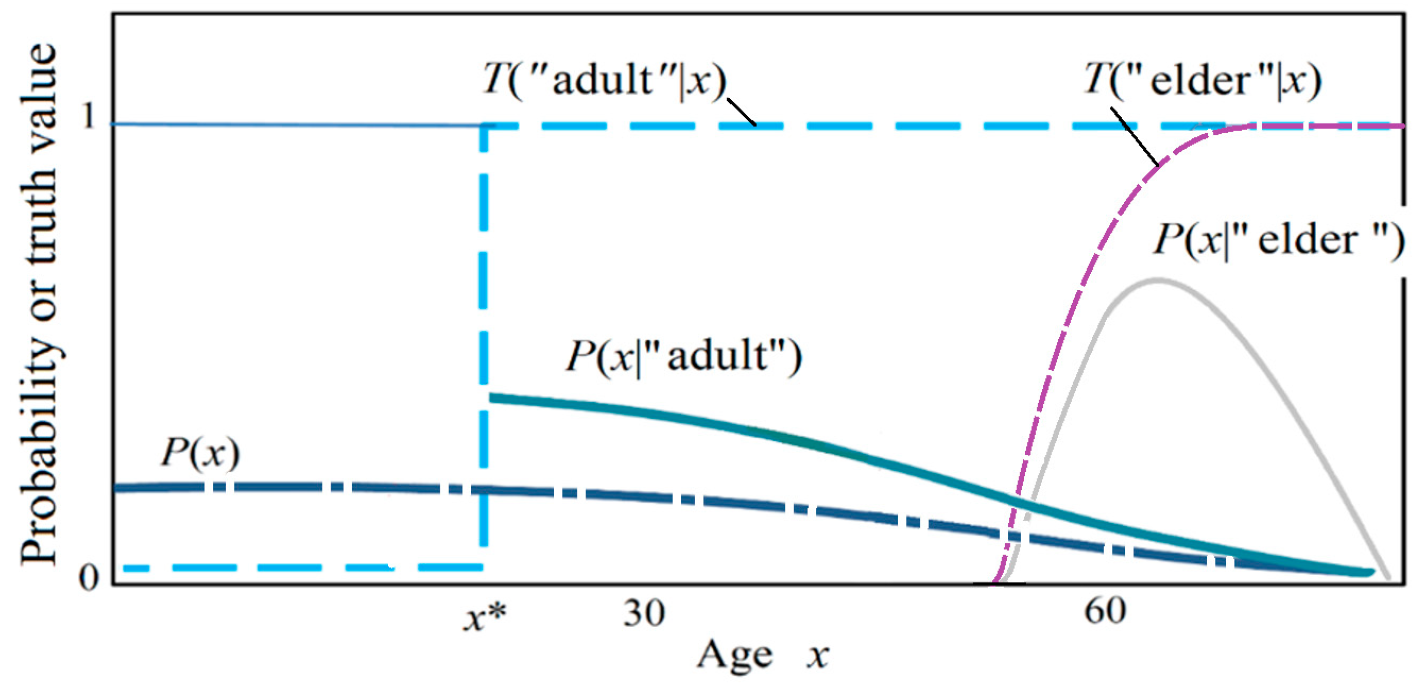
- For given age x, such as x = 30, the sum of the truth values of five labels may be bigger than 1.
- The logical probability of “adult” is related to the population age distribution P(x), which is a statistical probability distribution. Clearly, the logical probabilities of “adult” obtained from the door of a school and the door of a hospital must be different.
1.2. A Problem with the Extension of Logic: Can a Probability Function Be a Truth Function?
- The existing probability theories lack the methods used by the human brain (1) to find the extension of a label (an inductive method) and (2) to use the extension as the condition for reasoning or prediction (a deductive method).
- The TPF and the truth function are different, because a TPF is related to how many labels are used, whereas a truth function is not.
1.3. Distinguishing (Fuzzy) Truth Values and Logical Probabilities—Using Zadeh’s Fuzzy Set Theory
1.4. Can We Use Sampling Distributions to Optimize Truth Functions or Membership Functions?
1.5. Purpose, Methods, and Structure of This Paper
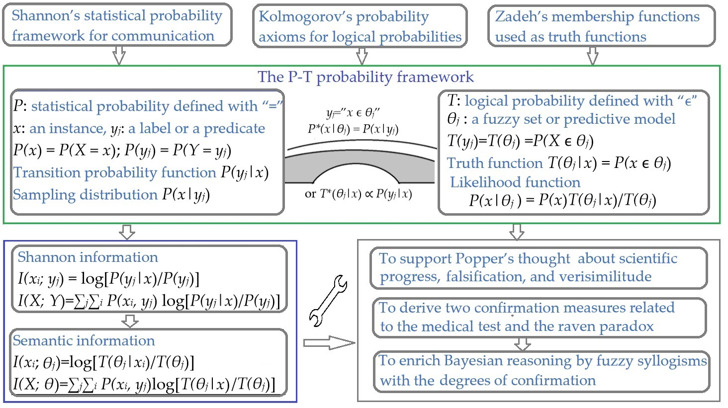
- using the statistical probability framework, e.g., the P probability framework, adopted by Shannon for electrocommunication as the foundation, adding Kolmogorov’s axioms (for logical probability) and Zadeh’s membership functions (as truth functions) to the framework,
- setting up the relationship between truth functions and likelihood functions by a new Bayes Theorem, called Bayes’ Theorem III, so that we can optimize truth functions (in logic) with sampling distributions (in statistics), and
- using the P–T probability framework and the semantic information Formulas (1) to express verisimilitude and testing severity and (2) to derive two practical confirmation measures and several new formulas to enrich Bayesian reasoning (including fuzzy syllogisms).
2. The P–T Probability Framework
2.1. The Probability Framework Adopted by Shannon for Electrocommunication
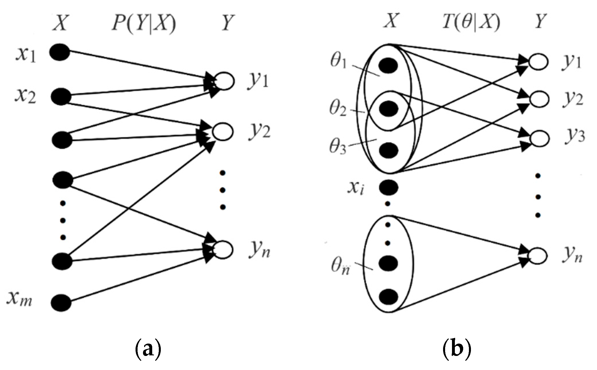
- X is a discrete random variable taking a value xϵU, whereUis the universe {x1, x2, …, xm}; P(xi) =P(X = xi) is the limit of the relative frequency of event X = xi. In the following applications, x represents an instance or a sample point.
- Y is a discrete random variable taking a value yϵV = {y1, y2, …, yn};P(yj) = P(Y = yj). In the following applications, y represents a label, hypothesis, or predicate.
- P(yj|x) = P(Y = yj|X = x) is a Transition Probability Function (TPF) (named by Shannon [3]).
2.2. The P–T Probability Framework for Semantic Communication
- The yj is a label or a hypothesis, yj(xi) is a proposition, and yj(x) is a propositional function. We also call yj or yj(x) a predicate. The θj is a fuzzy subset of universe U, which is used to explain the semantic meaning of a propositional function yj(x) = “x ϵ θj” = “x belongs to θj” = “x is in θj”. The θj is also treated as a model or a set of model parameters.
- A probability that is defined with “=“, such as P(yj) = P(Y = yj), is a statistical probability. A probability that is defined with “ϵ”, such as P(X ϵ θj), is a logical probability. To distinguish P(Y = yj) and P(X ϵ θj), we define T(yj) = T(θj) = P(X ϵ θj) as the logical probability of yj.
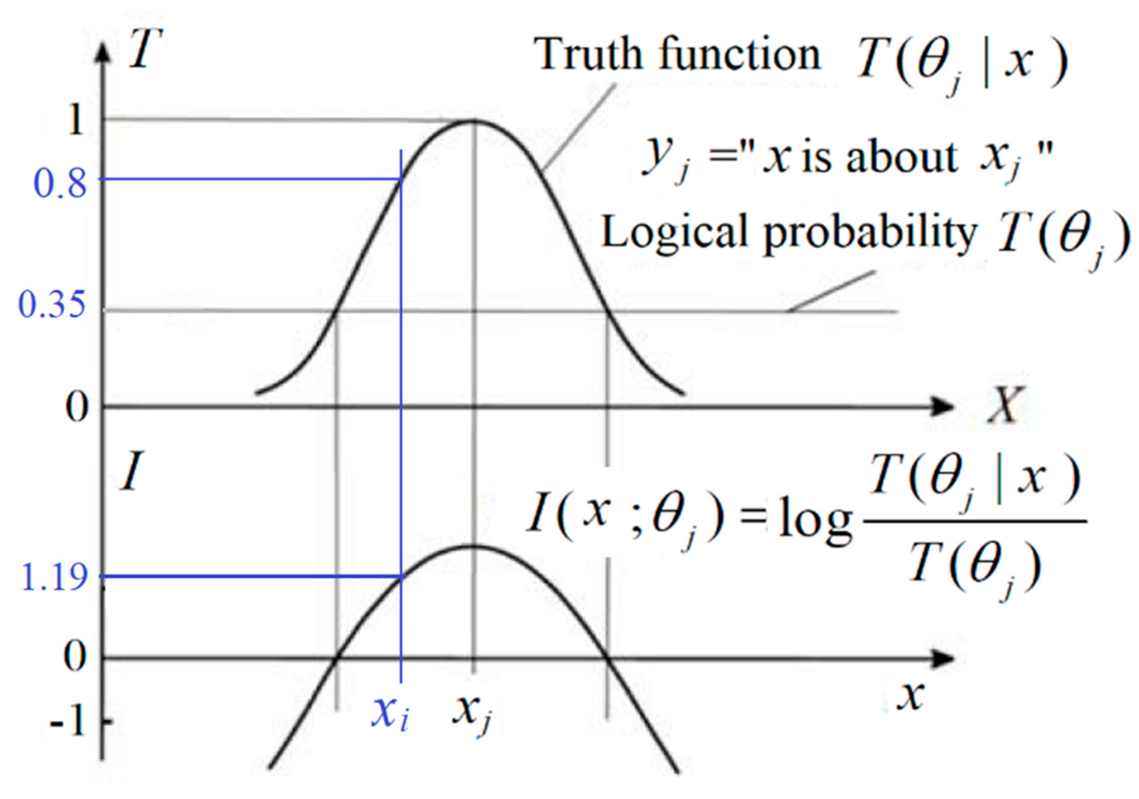
- T(yj|x) = T(θj|x) = P(x ϵ θj) = P(X ϵ θj|X = x) is the truth function of yj and the membership function of θj. It changes between 0 and 1, and its maximum is 1.
- The universe of θ only contains some subsets of 2U that form a partition of U, which means any two subsets in the universe are disjoint.
- The yj is always correctly selected.
2.3. Three Bayes’ Theorems
2.4. The Matching Relation between Statistical Probabilities and Logical Probabilities
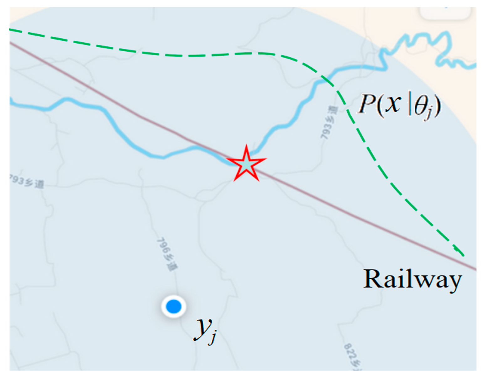
2.5. The Logical Probability and the Truth Function of a GPS Pointer or a Color Sense
3. The P–T Probability Framework for Semantic Communication, Statistical Learning, and Constraint Control
3.1. From Shannon’s Information Measure to the Semantic Information Measure
3.2. Optimizing Truth Functions and Classifications for Natural Language
3.3. Truth Functions Used as Distribution Constraint Functions for Random Events’ Control
- For given DCFs T(θj|x) (j = 1, 2, …, n) and P(x), when P(x|yj) = P(x|θj) = P(x)T(θj|x)/T(θj), the KL divergence I(X; yj) and Shannon’s mutual information I(X; Y) reach their minima; the effective control amount Ic(X; yj) reaches its maximum. If every set θj is crisp, I(X; yj) = −logT(θj) and I(X; Y) = −∑j P(yj)logT(θj).
- A rate-distortion function R(D) is equivalent to a rate-tolerance function R(Θ), and a semantic mutual information formula can express it with truth functions or DCFs (see Appendix B for details). However, an R(Θ) function may not be equivalent to an R(D) function, and hence, R(D) is a special case of R(Θ).
4. How the P–T probability Framework and the G Theory Support Popper’s Thought
4.1. How Popper’s Thought about Scientific Progresses is Supported by the Semantic Information Measure
“The amount of empirical information conveyed by a theory, or its empirical content, increases with its degree of falsifiability.”(p. 96)
“The logical probability of a statement is complementary to its degree of falsifiability: it increases with decreasing degree of falsifiability.”(p. 102)
“It characterizes as preferable the theory which tells us more; that is to say, the theory which contains the greater amount of experimental information or content; which is logically stronger; which has greater explanatory and predictive power; and which can therefore be more severely tested by comparing predicted facts with observations. In short, we prefer an interesting, daring, and highly informative theory to a trivial one.”.([45], p. 294)
4.2. How the Semantic Information Measure Supports Popper’s Falsification Thought
- Popper claims that scientific knowledge grows by repeating conjectures and refutations. Repeating conjectures should include adding auxiliary hypotheses.
- Falsification is not the aim. Falsifiability is only the demarcation criterion of scientific and non-scientific theories. The aim of science is to predict empirical facts with more information. Scientists hold a scientific theory depending on if it can convey more information than other theories. Therefore, being falsified does not means being given up.
- increasing the fuzziness or decreasing the predictive precision of the hypothesis to a proper level and
- reducing the degree of belief in a rule or a major premise.
4.3. For Verisimilitude: To Reconcile the Content Approach and the Likeness Approach
5. The P–T Probability Framework and the G Theory Are Used for Confirmation
5.1. The Purpose of Confirmation: Optimizing the Degrees of Belief in Major Premises for Uncertain Syllogisms
- The task of confirmation:
- Only major premises, such as “if the medical test is positive, then the tested person is infected” and “if x is a raven, then x is black”, need confirmation. The degrees of confirmation are between −1 and 1. A proposition, such as “Tom is elderly”, or a predicate, such as “x is elderly” (x is one of the given people), needs no confirmation. The truth function of the predicate reflects the semantic meaning of “elderly” and is determined by the definition or the idiomatic usage of “elderly”. The degree of belief in a proposition is a truth value, and that in a predicate is a logical probability. The truth value and the logical probability are between 0 and 1 instead of −1 and 1.
- The purpose of confirmation:
- The purpose of confirmation is not only for assessing hypotheses (major premises), but also for probability predictions or uncertain syllogisms. A syllogism needs a major premise. However, as pointed out by Hume and Popper, it is impossible to obtain an absolutely right major premise for an infinite universe by induction. However, it is possible to optimize the degree of belief in the major premise by the proportions of positive examples and counterexamples. The optimized degree of belief is the degree of confirmation. Using a degree of confirmation, we can make an uncertain or fuzzy syllogism. Therefore, confirmation is an important link in scientific reasoning according to experience.
- The method of confirmation:
- I do not directly define a confirmation measure, as most researchers do. I derive the confirmation measures by optimizing the degree of belief in a major premise with the maximum semantic information criterion or the maximum likelihood criterion. This method is also the method of statistical learning, where the evidence is a sample.
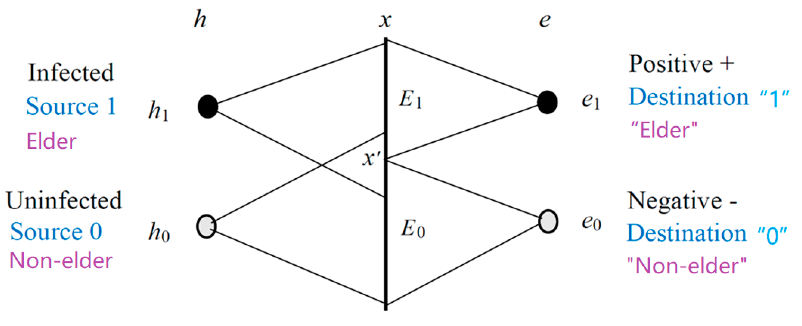
5.2. Channel Confirmation Measure b* for Assessing a Classification as a Channel
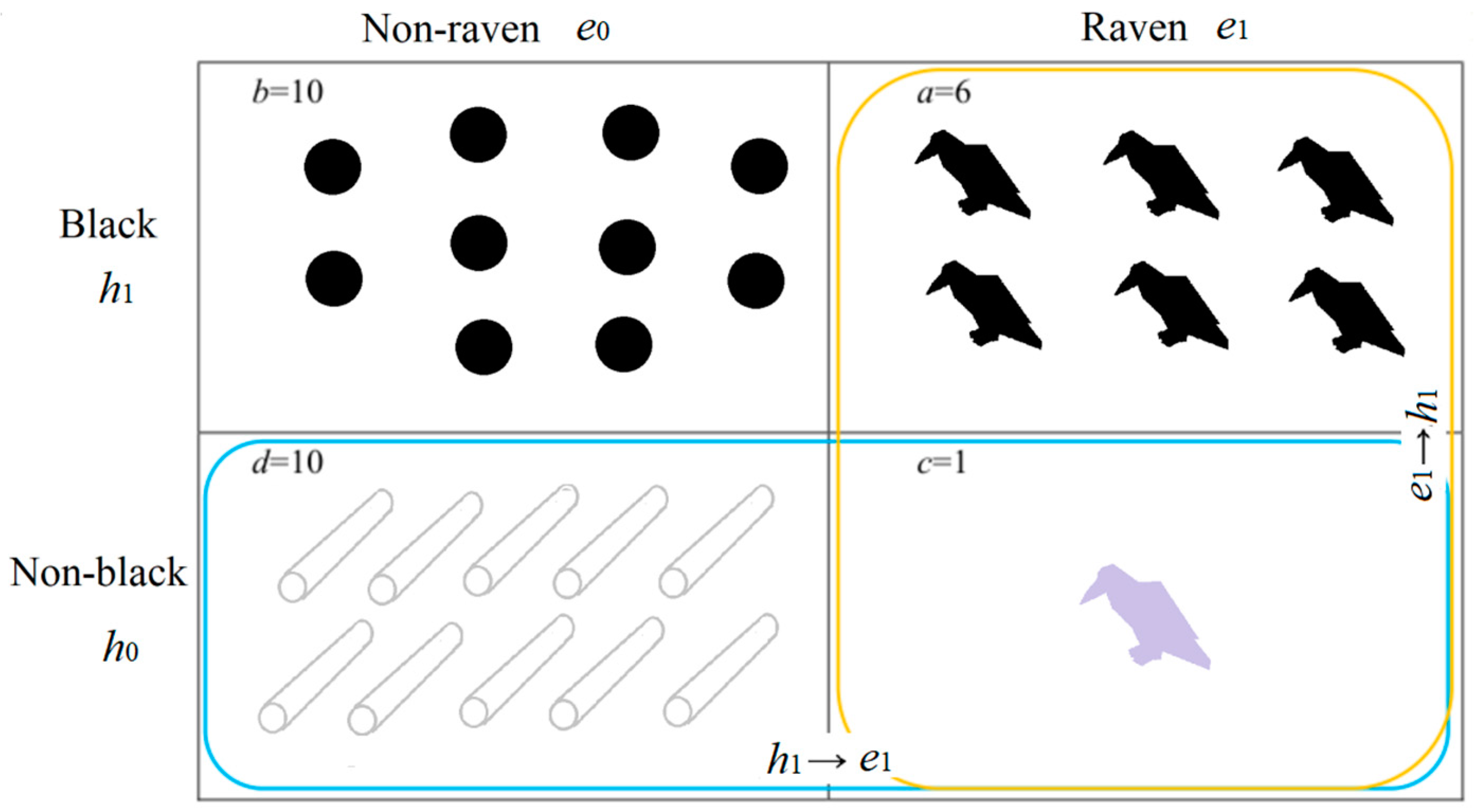
5.3. Prediction Confirmation Measure c* for Clarifying the Raven Paradox
5.4. How Confirmation Measures F, b*, and c* are Compatible with Popper’s Falsification Thought
6. Induction, Reasoning, Fuzzy Syllogisms, and Fuzzy Logic
6.1. Viewing Induction from the New Perspective
- induction for probability predictions: to optimize likelihood functions with sampling distributions,
- induction for the semantic meanings or the extensions of labels: to optimize truth functions with sampling distributions, and
- induction for the degrees of confirmation of major premises: to optimize the degrees of belief in major premises with the proportions of positive examples and counterexamples after classifications.
6.2. The Different Forms of Bayesian Reasoning as Syllogisms
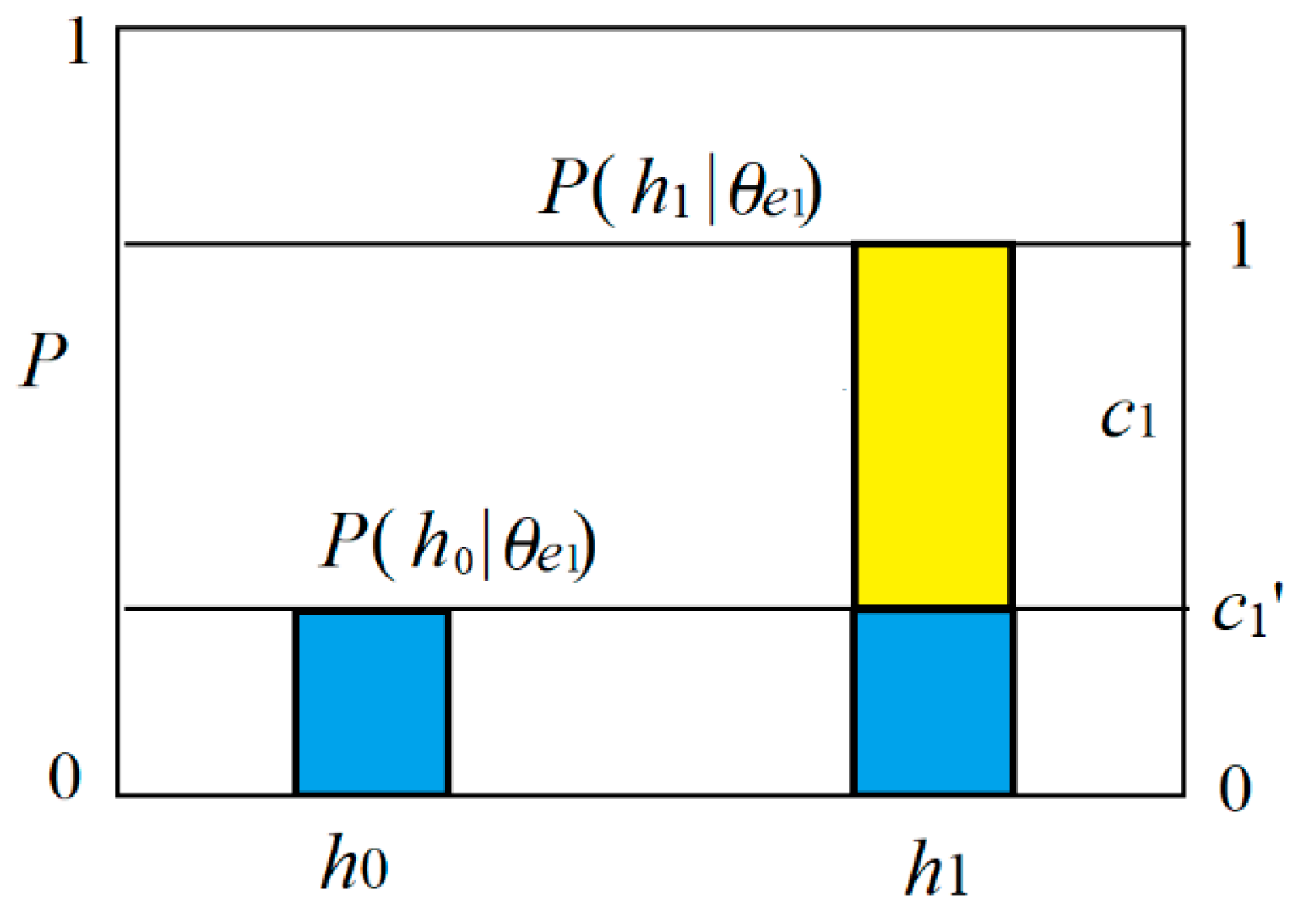
- The major premise is b*(e1→h1) = b1*
- The minor premise is e1 with P(h),
- The consequence is P(h|θe1) = P(h1)/[P(h1) + (1 − b1*)P(h0)] = P(h1)/[1 − b1*P(h0)].
6.3. Fuzzy Logic: Expectations and Problems
7. Discussions
7.1. How the P–T Probability Framework has Been Tested by Its Applications to Theories
- two types of reasoning with Bayes’ Theorem III,
- Logical Bayesian Inference from sampling distributions to optimized truth functions, and
- fuzzy syllogisms with the degrees of confirmation of major premises.
7.2. How to Extend Logic to the Probability Theory?
7.3. Comparing the Truth Function with Fisher’s Inverse Probability Function
- We can use an optimized truth function T*(θj|x) to make probability prediction for different P(x) as well as we use P(yj|x) or P(θj|x).
- We can train a truth function with parameters by a sample with a small size as well as we train a likelihood function.
- The truth function can indicate the semantic meaning of a hypothesis or the extension of a label.It is also the membership function, which is suitable for classification.
- To train a truth function T(θj|x), we only need P(x) and P(x|yj), without needing P(yj) or P(θj).
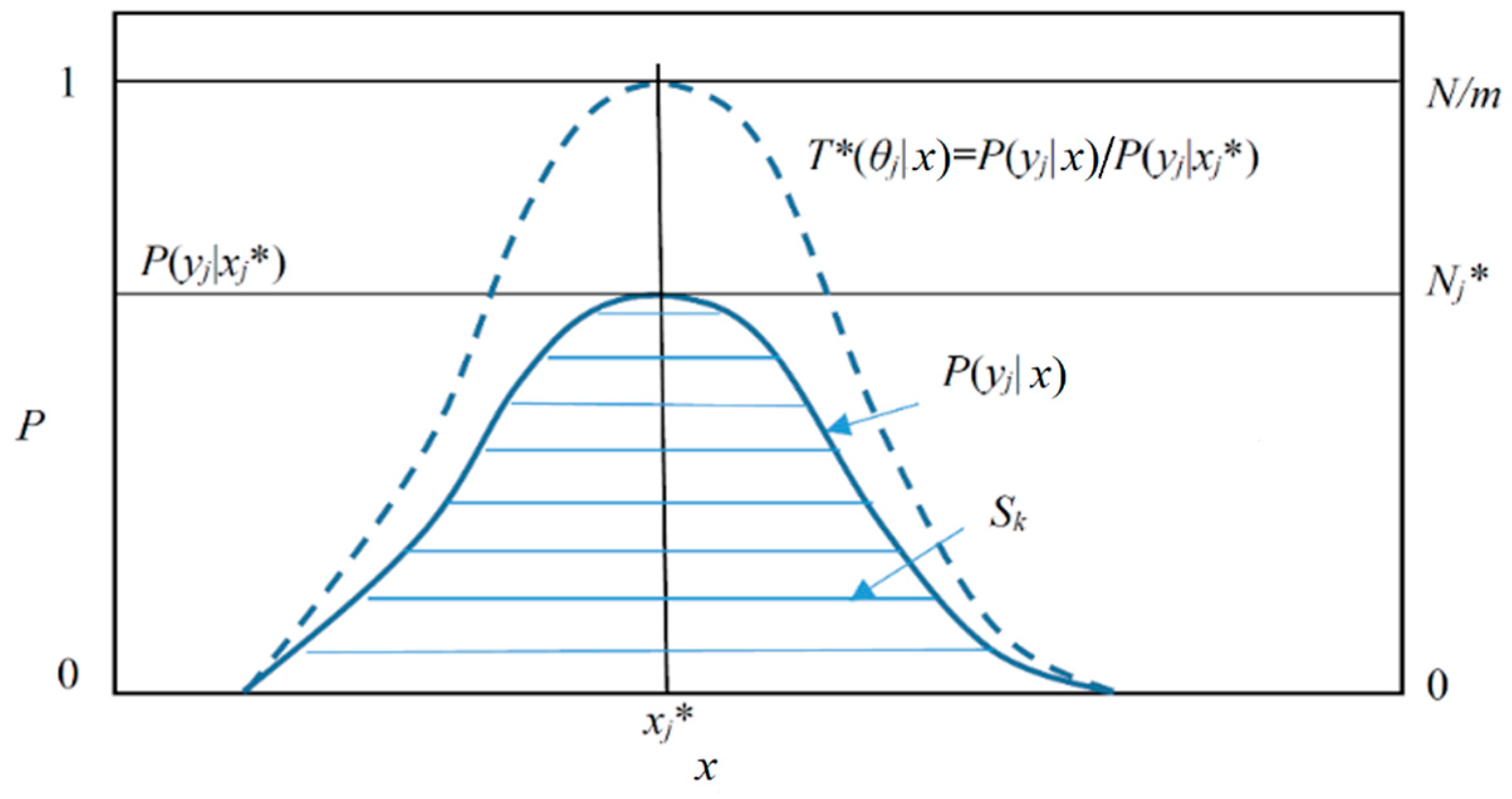
- Letting T*(θj|x)∝P(yj|x), we can bridge statistics and logic.
7.4. Answers to Some Questions
7.5. Some Issues That Need Further Studies
- The human brain thinks using the extensions (or denotations) of concepts more than interdependencies. A truth function indicates the (fuzzy) extension of a label and reflects the semantic meaning of the label; Bayes’ Theorem III expresses the reasoning with the extension.
- The new confirmation methods and the fuzzy syllogisms can express the induction and the reasoning with degrees of belief that the human brain uses, and the reasoning is compatible with statistical reasoning.
- The Boltzmann distribution has been applied to the Boltzmann machine [71] for machine learning. With the help of the semantic Bayes formula and the semantic information methods, we can better understand this distribution and the Regularized Least Square criterion related to information.
8. Conclusions
Funding
Acknowledgments
Conflicts of Interest
Appendix A. The Proof of Bayes’ Theorem III
Appendix B. A R(D) Function is Equal to a R(Θ) Function with Truth Functions
Appendix C. The Relationship between Information and Thermodynamic Entropy [14]
Appendix D. The Derivation for b1*
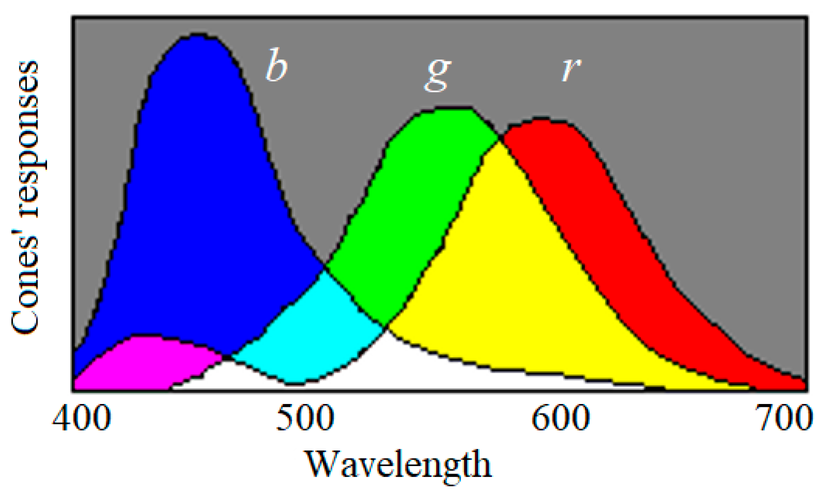
Appendix E. Illustrating the Fuzzy Logic in the Decoding Model of Color Vision

Appendix F. To Prove P(q|p) ≤ P(p => q)
References
- Galavotti, M.C. The Interpretation of Probability: Still an Open Issue? Philosophies 2017, 2, 20. [Google Scholar] [CrossRef]
- Hájek, A. Interpretations of probability. In the Stanford Encyclopedia of Philosophy (Fall 2019 Edition); Zalta, E.N., Ed.; Available online: https://plato.stanford.edu/archives/fall2019/entries/probability-interpret/ (accessed on 17 June 2020).
- Shannon, C.E. A mathematical theory of communication. Bell Syst. Tech. J. 1948, 27, 379–423. [Google Scholar] [CrossRef]
- Fisher, R.A. On the mathematical foundations of theoretical statistics. Philos. Trans. R. Soc. 1922, 222, 309–368. [Google Scholar]
- Fienberg, S.E. When did Bayesian Inference become “Bayesian”? Bayesian Anal. 2006, 1, 1–40. [Google Scholar] [CrossRef]
- Popper, K.R. The propensity interpretation of the calculus of probability and the quantum theory. In the Colston Papers No 9; Körner, S., Ed.; Butterworth Scientific Publications: London, UK, 1957; pp. 65–70. [Google Scholar]
- Popper, K. Logik Der Forschung: Zur Erkenntnistheorie Der Modernen Naturwissenschaft; Springer: Vienna, Austria, 1935; English translation: The Logic of Scientific Discovery; Routledge Classic: London, UK; New York, NY, USA, 2002. [Google Scholar]
- Carnap, R. The two concepts of Probability: The problem of probability. Philos. Phenomenol. Res. 1945, 5, 513–532. [Google Scholar] [CrossRef]
- Reichenbach, H. The Theory of Probability; University of California Press: Berkeley, CA, USA, 1949. [Google Scholar]
- Kolmogorov, A.N. Grundbegriffe der Wahrscheinlichkeitrechnung; Ergebnisse Der Mathematik (1933); Translated as Foundations of Probability; Chelsea Publishing Company: New York, NY, USA, 1950. [Google Scholar]
- Greco, S.; Slowiński, R.; Szczech, I. Measures of rule interestingness in various perspectives of confirmation. Inf. Sci. 2016, 346, 216–235. [Google Scholar] [CrossRef]
- Lu, C. Semantic Information G Theory and Logical Bayesian Inference for Machine Learning. Information 2019, 10, 261. Available online: https://www.mdpi.com/2078-2489/10/8/261 (accessed on 10 September 2020). [CrossRef]
- Lu, C. Shannon equations’ reform and applications. BUSEFAL 1990, 44, 45–52. Available online: https://www.listic.univ-smb.fr/production-scientifique/revue-busefal/version-electronique/ebusefal-44/ (accessed on 5 March 2019).
- Lu, C. A Generalized Information Theory; China Science and Technology University Press: Hefei, China, 1993; ISBN 7-312-00501-2. (In Chinese) [Google Scholar]
- Lu, C. A generalization of Shannon’s information theory. Int. J. Gen. Syst. 1999, 28, 453–490. [Google Scholar] [CrossRef]
- Jaynes, E.T. Probability Theory: The Logic of Science; Bretthorst, G.L., Ed.; Cambridge University Press: Cambridge, UK, 2003. [Google Scholar]
- Dubois, D.; Prade, H. Possibility theory, probability theory and multiple-valued logics: A clarification. Ann. Math. Artif. Intell. 2001, 32, 35–66. [Google Scholar] [CrossRef]
- Carnap, R. Logical Foundations of Probability, 2nd ed.; University of Chicago Press: Chicago, IL, USA, 1962. [Google Scholar]
- Zadeh, L.A. Fuzzy sets. Inf. Control 1965, 8, 338–353. [Google Scholar] [CrossRef]
- Zadeh, L.A. Probability measures of fuzzy events. J. Math. Anal. Appl. 1986, 23, 421–427. [Google Scholar]
- Zadeh, L.A. Fuzzy set theory and probability theory: What is the relationship? In International Encyclopedia of Statistical Science; Lovric, M., Ed.; Springer: Berlin/Heidelberg, Germany, 2011. [Google Scholar]
- Wang, P.Z. From the fuzzy statistics to the falling random subsets. In Advances in Fuzzy Sets, Possibility Theory and Applications; Wang, P.P., Ed.; Plenum Press: New York, NY, USA, 1983; pp. 81–96. [Google Scholar]
- Wang, P.Z. Fuzzy Sets and Falling Shadows of Random Set; Beijing Normal University Press: Beijing, China, 1985. (In Chinese) [Google Scholar]
- Keynes, J.M. A Treatise on Probability; Macmillan and Co.: London, UK, 1921. [Google Scholar]
- Demey, L.; Kooi, B.; Sack, J. Logic and probability. In The Stanford Encyclopedia of Philosophy (Summer 2019 Edition); Edward, N.Z., Ed.; Available online: https://plato.stanford.edu/archives/sum2019/entries/logic-probability/ (accessed on 17 June 2020).
- Adams, E.W. A Primer of Probability Logic; CSLI Publications: Stanford, CA, USA, 1998. [Google Scholar]
- Dubois, D.; Prade, H. Fuzzy sets and probability: Misunderstandings, bridges and gaps. In Proceedings of the 1993 Second IEEE International Conference on Fuzzy Systems, San Francisco, CA, USA, 28 March–1 April 1993; Volume 2, pp. 1059–1068. [Google Scholar] [CrossRef]
- Coletti, G.; Scozzafava, R. Conditional probability, fuzzy sets, and possibility: A unifying view. Fuzzy Sets Syst. 2004, 144, 227–249. [Google Scholar]
- Gao, Q.; Gao, X.; Hu, Y. A uniform definition of fuzzy set theory and the fundamentals of probability theory. J. Dalian Univ. Technol. 2006, 46, 141–150. (In Chinese) [Google Scholar]
- von Mises, R. Probability, Statistics and Truth, 2nd ed.; George Allen and Unwin Ltd.: London, UK, 1957. [Google Scholar]
- Tarski, A. The semantic conception of truth: And the foundations of semantics. Philos. Phenomenol. Res. 1994, 4, 341–376. [Google Scholar] [CrossRef]
- Davidson, D. Truth and meaning. Synthese 1967, 17, 304–323. [Google Scholar] [CrossRef]
- Carnap, R.; Bar-Hillel, Y. An Outline of a Theory of Semantic Information; Technical Report No. 247; Research Lab. of Electronics, MIT: Cambridge, MA, USA, 1952. [Google Scholar]
- Bayes, T.; Price, R. An essay towards solving a problem in the doctrine of chance. Philos. Trans. R. Soc. Lond. 1763, 53, 370–418. [Google Scholar]
- Wittgenstein, L. Philosophical Investigations; Basil Blackwell Ltd.: Oxford, UK, 1958. [Google Scholar]
- Wikipedia contributors, Dempster–Shafer theory. In Wikipedia, the Free Encyclopedia; 29 May 2020; Available online: https://en.wikipedia.org/wiki/Dempster%E2%80%93Shafer_theory (accessed on 18 June 2020).
- Lu, C. The third kind of Bayes’ Theorem links membership functions to likelihood functions and sampling distributions. In Cognitive Systems and Signal Processing; Sun, F., Liu, H., Hu, D., Eds.; ICCSIP 2018, Communications in Computer and Information Science, vol 1006; Springer: Singapore, 2019; pp. 268–280. [Google Scholar]
- Floridi, L. Semantic conceptions of information. In Stanford Encyclopedia of Philosophy; Stanford University: Stanford, CA, USA, 2005; Available online: http://seop.illc.uva.nl/entries/information-semantic/ (accessed on 17 June 2020).
- Shannon, C.E. Coding theorems for a discrete source with a fidelity criterion. IRE Nat. Conv. Rec. 1959, 4, 142–163. [Google Scholar]
- Zhang, M.L.; Li, Y.K.; Liu, X.Y.; Geng, X. Binary relevance for multi-label learning: An overview. Front. Comput. Sci. 2018, 12, 191–202. [Google Scholar]
- Lu, C. GPS information and rate-tolerance and its relationships with rate distortion and complexity distortions. J. Chengdu Univ. Inf. Technol. 2012, 6, 27–32. (In Chinese) [Google Scholar]
- Sow, D.M. Complexity Distortion Theory. IEEE Trans. Inf. Theory 2003, 49, 604–609. [Google Scholar] [CrossRef]
- Berger, T. Rate Distortion Theory; Prentice-Hall: Enklewood Cliffs, NJ, USA, 1971. [Google Scholar]
- Wikipedia contributors, Boltzmann distribution. In Wikipedia, the Free Encyclopedia; 5 August 2020; Available online: https://en.wikipedia.org/wiki/Boltzmann_distribution (accessed on 12 August 2020).
- Popper, K. Conjectures and Refutations, 1st ed.; Routledge: London, UK; New York, NY, USA, 2002. [Google Scholar]
- Zhong, Y.X. A theory of semantic information. China Commun. 2017, 14, 1–17. [Google Scholar] [CrossRef]
- Klir, G. Generalized information theory. Fuzzy Sets Syst. 1991, 40, 127–142. [Google Scholar] [CrossRef]
- Lakatos, I. Falsification and the methodology of scientific research programmes. In Can Theories be Refuted? Synthese Library; Harding, S.G., Ed.; Springer: Dordrecht, The Netherlands, 1976; Volume 81. [Google Scholar]
- Popper, K. Realism and the Aim of Science; Bartley, W.W., III, Ed.; Routledge: New York, NY, USA, 1983. [Google Scholar]
- Lakatos, I. Popper on demarcation and induction. In the Philosophy of Karl Popper; Schilpp, P.A., Ed.; Open Court: La Salle, IL, USA, 1974; pp. 241–273. [Google Scholar]
- Tichý, P. On Popper’s definitions of verisimilitude. Br. J. Philos. Sci. 1974, 25, 155–160. [Google Scholar] [CrossRef]
- Oddie, G. Truthlikeness, the Stanford Encyclopedia of Philosophy (Winter 2016 Edition); Zalta, E.N., Ed.; Available online: https://plato.stanford.edu/archives/win2016/entries/truthlikeness/ (accessed on 18 May 2020).
- Zwart, S.D.; Franssen, M. An impossibility theorem for verisimilitude. Synthese 2007, 158, 75–92. Available online: https://doi.org/10.1007/s11229-006-9051-y (accessed on 10 September 2020). [CrossRef][Green Version]
- Eells, E.; Fitelson, B. Symmetries and asymmetries in evidential support. Philos. Stud. 2002, 107, 129–142. [Google Scholar] [CrossRef]
- Kemeny, J.; Oppenheim, P. Degrees of factual support. Philos. Sci. 1952, 19, 307–324. [Google Scholar] [CrossRef]
- Huber, F. What Is the Point of Confirmation? Philos. Sci. 2005, 72, 1146–1159. [Google Scholar] [CrossRef]
- Hawthorne, J. Inductive Logic. In The Stanford Encyclopedia of Philosophy (Spring 2018 Edition); Edward, N.Z., Ed.; Available online: https://plato.stanford.edu/archives/spr2018/entries/logic-inductive/ (accessed on 18 May 2020).
- Lu, C. Channels’ confirmation and predictions’ confirmation: From the medical test to the raven paradox. Entropy 2020, 22, 384. Available online: https://www.mdpi.com/1099-4300/22/4/384 (accessed on 10 September 2020). [CrossRef]
- Hempel, C.G. Studies in the logic of confirmation. Mind 1945, 54, 1–26. [Google Scholar] [CrossRef]
- Nicod, J. Le Problème Logique De L’induction; Alcan: Paris, France, 1924; p. 219, English translation: The logical problem of induction. In Foundations of Geometry and Induction; Routledge: London, UK, 2000. [Google Scholar]
- Scheffler, I.; Goodman, N.J. Selective confirmation and the ravens: A reply to Foster. J. Philos. 1972, 69, 78–83. [Google Scholar] [CrossRef]
- Fitelson, B.; Hawthorne, J. How Bayesian confirmation theory handles the paradox of the ravens. In the Place of Probability in Science; Eells, E., Fetzer, J., Eds.; Springer: Dordrecht, Germany, 2010; pp. 247–276. [Google Scholar]
- Wikipedia Contributors, Syllogism. Wikipedia, the Free Encyclopedia. Available online: https://en.wikipedia.org/w/index.php?title=Syllogism&oldid=958696904 (accessed on 20 May 2020).
- Wang, P.Z.; Zhang, H.M.; Ma, X.W.; Xu, W. Fuzzy set-operations represented by falling shadow theory. In Fuzzy Engineering toward Human Friendly Systems, Proceedings of the International Fuzzy Engineering Symposium’91, Yokohama, Japan, 13–15 November 1991; IOS Press: Amsterdam, The Netherlands, 1991; Volume 1, pp. 82–90. [Google Scholar]
- Lu, C. Decoding model of color vision and verifications. Acta Opt. Sin. 1989, 9, 158–163. (In Chinese) [Google Scholar]
- Lu, C. B-fuzzy quasi-Boolean algebra and a generalize mutual entropy formula. Fuzzy Syst. Math. 1991, 5, 76–80. (In Chinese) [Google Scholar]
- CIELAB. Symmetric Colour Vision Model, CIELAB and Colour Information Technology. 2006. Available online: http://130.149.60.45/~farbmetrik/A/FI06E.PDF (accessed on 10 September 2020).
- Lu, C. Explaining color evolution, color blindness, and color recognition by the decoding model of color vision. In Proceedings of the 11th IFIP TC 12 International Conference, IIP 2020, Hangzhou, China, 3–6 July 2020; Shi, Z., Vadera, S., Chang, E., Eds.; Springer: Cham, Switzerland, 2020; pp. 287–298. Available online: https://www.springer.com/gp/book/9783030469306 (accessed on 10 September 2020).
- Guo, S.Z. Principle of Fuzzy Mathematical Analysis Based on Structured Element; Northeast University Press: Shenyang, Chine, 2004. (In Chinese) [Google Scholar]
- Froese, T.; Taguchi, S. The Problem of Meaning in AI and Robotics: Still with Us after All These Years. Philosophies 2019, 4, 14. [Google Scholar] [CrossRef]
- Wikipedia contributors, Boltzmann machine. Wikipedia, the Free Encyclopedia. Available online: https://en.wikipedia.org/wiki/Boltzmann_machine (accessed on 10 August 2020).


| e0 | e1 | |
|---|---|---|
| h1 | b | a |
| h0 | d | c |
| e0 (Negative) | e1 (Positive) | |
|---|---|---|
| h1 (Infected) | P(e0|h1) = b/(a + b) | P(e1|h1) = a/(a + b) |
| h0 (Uninfected) | P(e0|h0) = d/(c + d) | P(e1|h0) = c/(c + d) |
| e0 (Negative) | e1 (Positive) | |
|---|---|---|
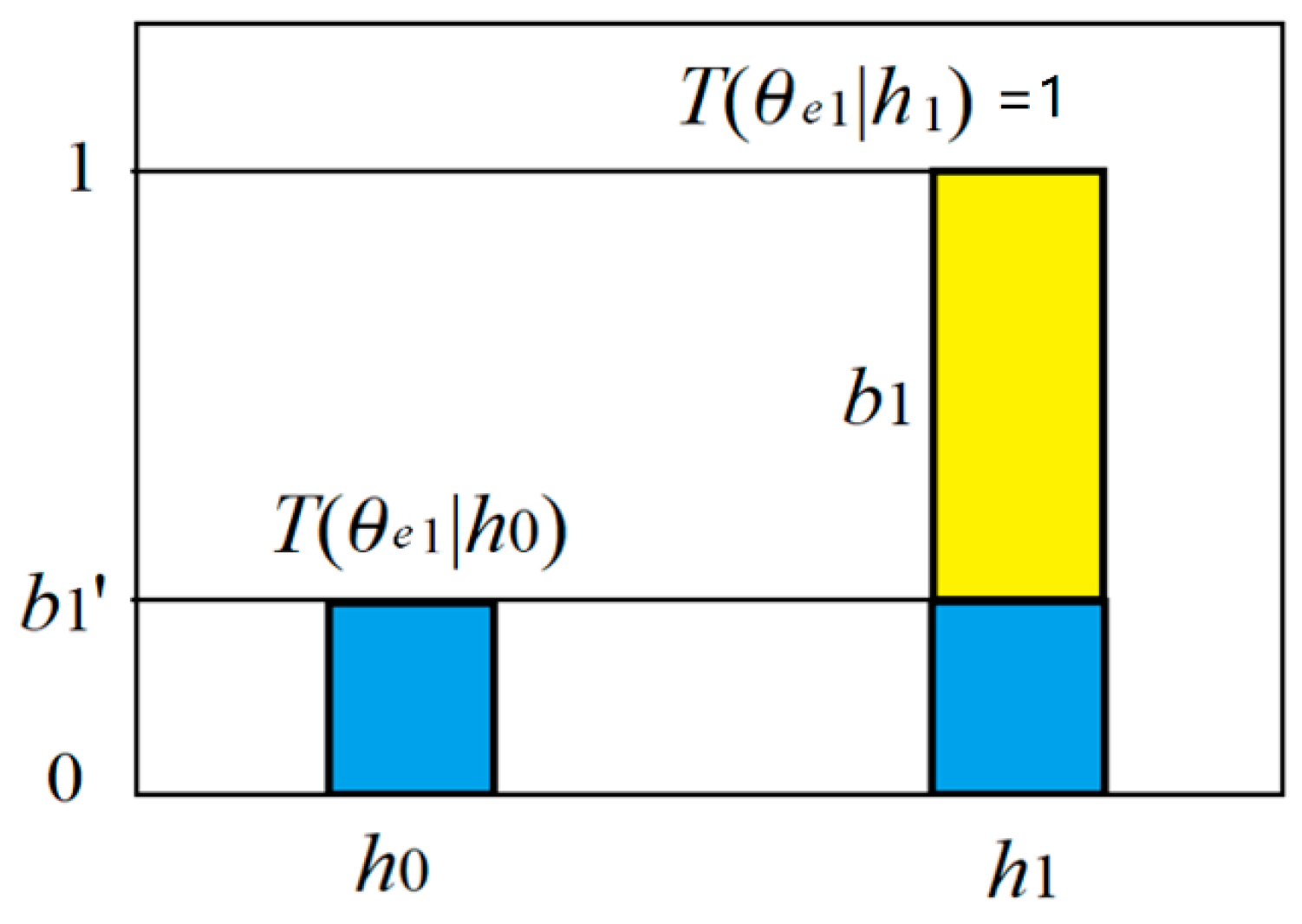
| h1 (infected) | T(θe0|h1) = b0′ | T(θe1|h1) = 1 |
| h0 (uninfected) | T(θe0|h0) = 1 | T(θe1|h0) = b1′ |
| Reasoning between/with | Major Premise or Model | Minor Premise or Evidence | Consequence | Interpretation |
|---|---|---|---|---|
| Between two instances | P(yj|x) | xi (X = xi) | P(yj|xi) | Conditional SP |
| yj, P(x) | P(x|yj) = P(x)P(yj|x)/P(yj) P(yj) = ∑iP(yj|xi) P(xi) | Bayes’ Theorem II (Bayes’ prediction) | ||
| Between two sets | T(θ2|θ) | y1 (is true) | T(θ2|θ1) | Conditional LP |
| y2, T(θ) | T(θ|θ2) = T(θ2|θ)T(θ)/T(θ2), T(θ2) = T(θ2|θ)T(θ) + T(θ2|θ’)T(θ’) | Bayes’ Theorem I (θ’ is the complement of θ) | ||
| Between an instance and a set (or model) | T(θj|x) | X = xi or P(x) | T(θj|xi) or T(θj) = ∑iT(θj|xi)P(xi) | Truth value and logical probability |
| yj is true, P(x) | P(x|θj) = P(x)T(θj|x)/T(θj), T(θj) = ∑iT(θj|xi)P(xi) | The semantic Bayes prediction in Bayes’ Theorem III | ||
| P(x|θj) | xi or Dj | P(xi|θj) or P(Dj|θj) | Likelihood | |
| P(x) | T(θj|x) = [P(x|θj)/P(x)]/max[P(x|θj)/P(x)] | Inference in Bayes’ Theorem III | ||
| Induction: with sampling distributions to train predictive models | P(x|θj) | P(x|yj) | P*(x|θj) (optimized P(x|θj) with P(x|yj)) | Likelihood Inference |
| P(x|θ) and P(θ) | P(x|y) or D | P(θ|D) = P(θ)P(D|θ)/ ∑j P(θj)P(D|θj) | Bayesian Inference | |
| T(θj|xj) | P(x|yj) and P(x) | T*(θj|x) = P(x|yj)/P(x)/max[P(x|yj)/P(x)] = P(yj|x)/max[P(yj|x)] | Logical Bayesian Inference | |
| With degree of channel confirmation | b1* = b*(e1→h1) > 0 | h or P(h) | T(θe1|h1) = 1, T(θe1|h0) = 1 − |b1*|; T(θe1) = P(h1) + (1 − b1*)P(h0) | Truth values and logical probability |
| e1 (e1 is true), P(h) | P(h1|θe1) = P(h1)/T(θe1), P(h0|θe1) = (1 − b1*)P(h0)/T(θe1); | A fuzzy syllogism with b* | ||
| With degree of prediction confirmation | c1* = c*(e1→h1) > 0 | e1 (e1 is true) | P(h1|θe1) = 1/(2 − c1*), P(h0|θe1) = (1 − c1*)/(2 − c1*) | A fuzzy syllogism with c* |
© 2020 by the author. Licensee MDPI, Basel, Switzerland. This article is an open access article distributed under the terms and conditions of the Creative Commons Attribution (CC BY) license (http://creativecommons.org/licenses/by/4.0/).
Share and Cite
Lu, C. The P–T Probability Framework for Semantic Communication, Falsification, Confirmation, and Bayesian Reasoning. Philosophies 2020, 5, 25. https://doi.org/10.3390/philosophies5040025
Lu C. The P–T Probability Framework for Semantic Communication, Falsification, Confirmation, and Bayesian Reasoning. Philosophies. 2020; 5(4):25. https://doi.org/10.3390/philosophies5040025
Chicago/Turabian StyleLu, Chenguang. 2020. "The P–T Probability Framework for Semantic Communication, Falsification, Confirmation, and Bayesian Reasoning" Philosophies 5, no. 4: 25. https://doi.org/10.3390/philosophies5040025
APA StyleLu, C. (2020). The P–T Probability Framework for Semantic Communication, Falsification, Confirmation, and Bayesian Reasoning. Philosophies, 5(4), 25. https://doi.org/10.3390/philosophies5040025