
Binarization of Metaheuristics: Is the Transfer Function Really Important?

 ,
,  , ,
, ,  and
and
Abstract
:1. Introduction
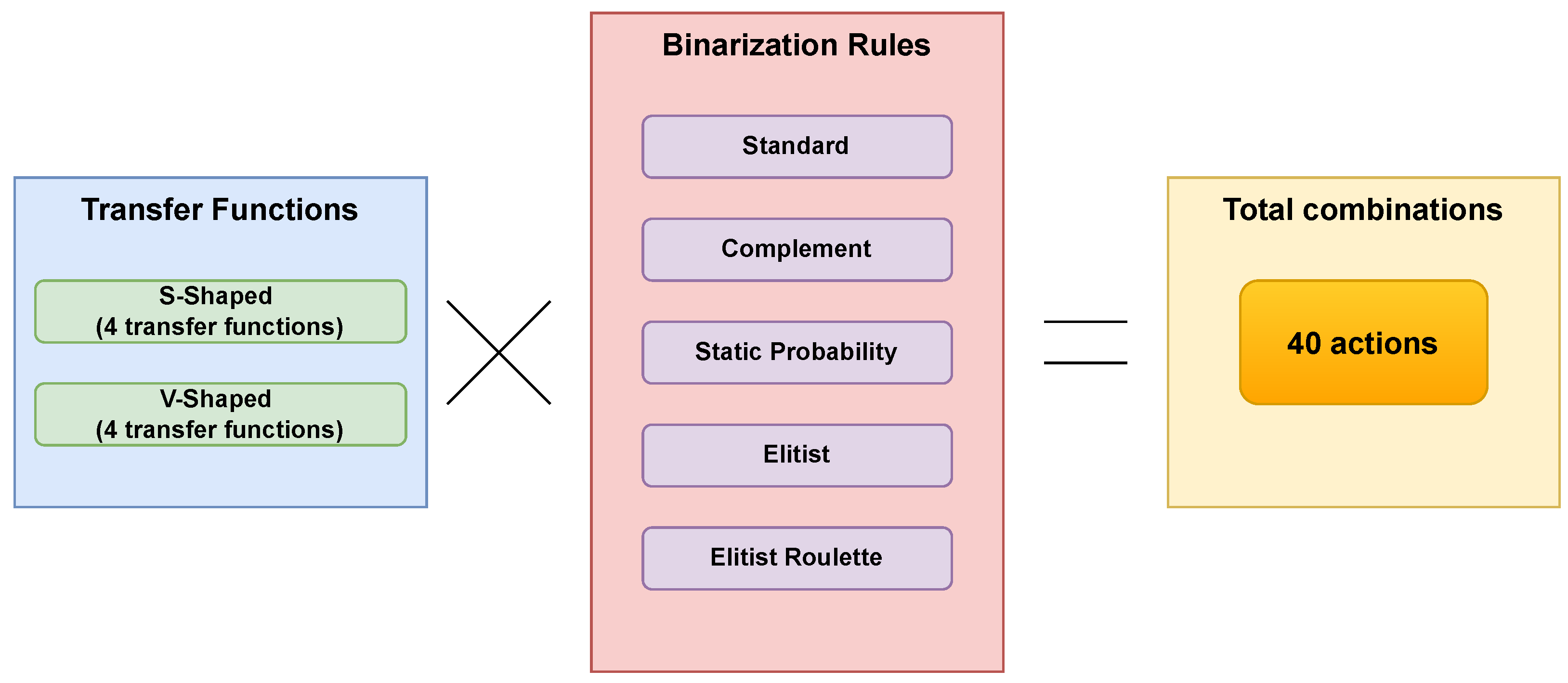
- Evaluate different sets of transfer functions and binarization rules.
- Explore the importance of binarization rules compared to transfer functions.
- Compare the results in three different and complex metaheuristics.
- Conduct a comprehensive comparison of the results obtained by solving the set covering problem.
2. Related Work
2.1. Continuous Metaheuristics to Solve Combinatorial Problems
2.2. Two-Step Techniques
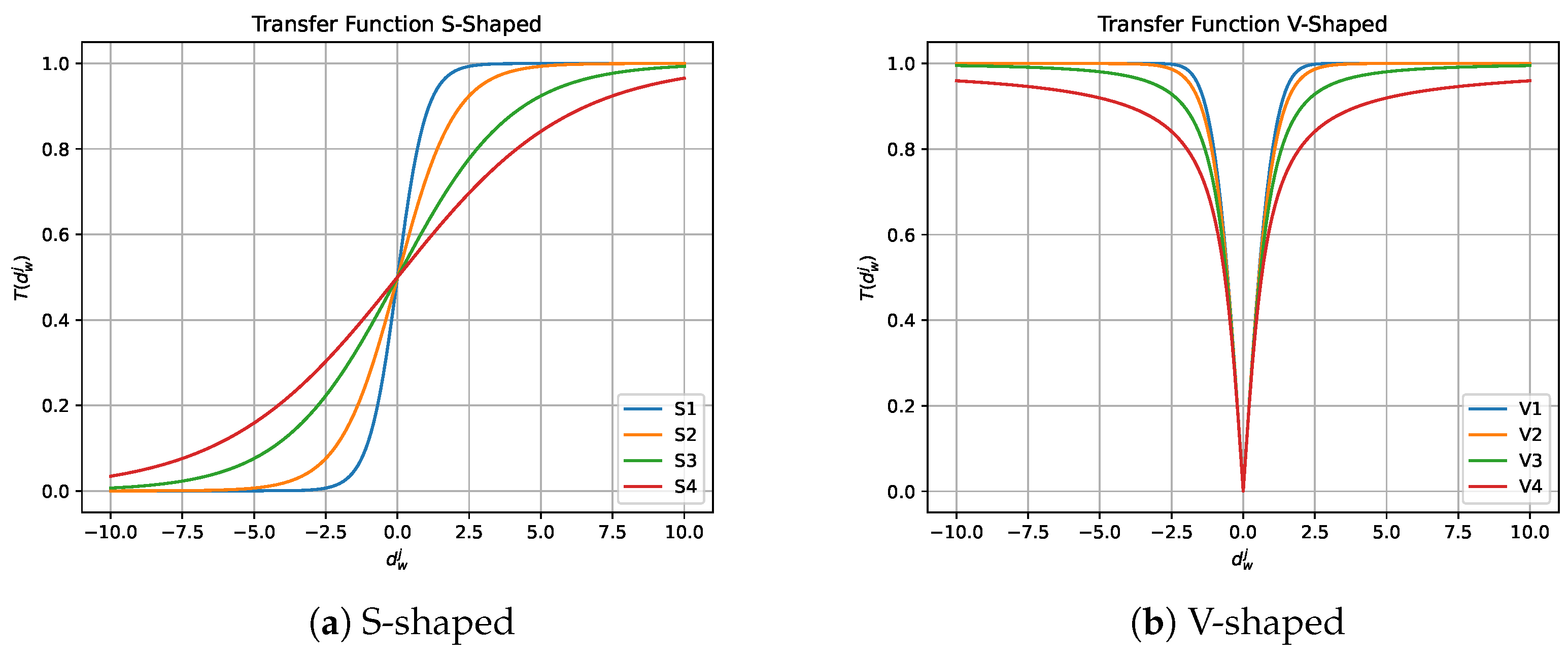
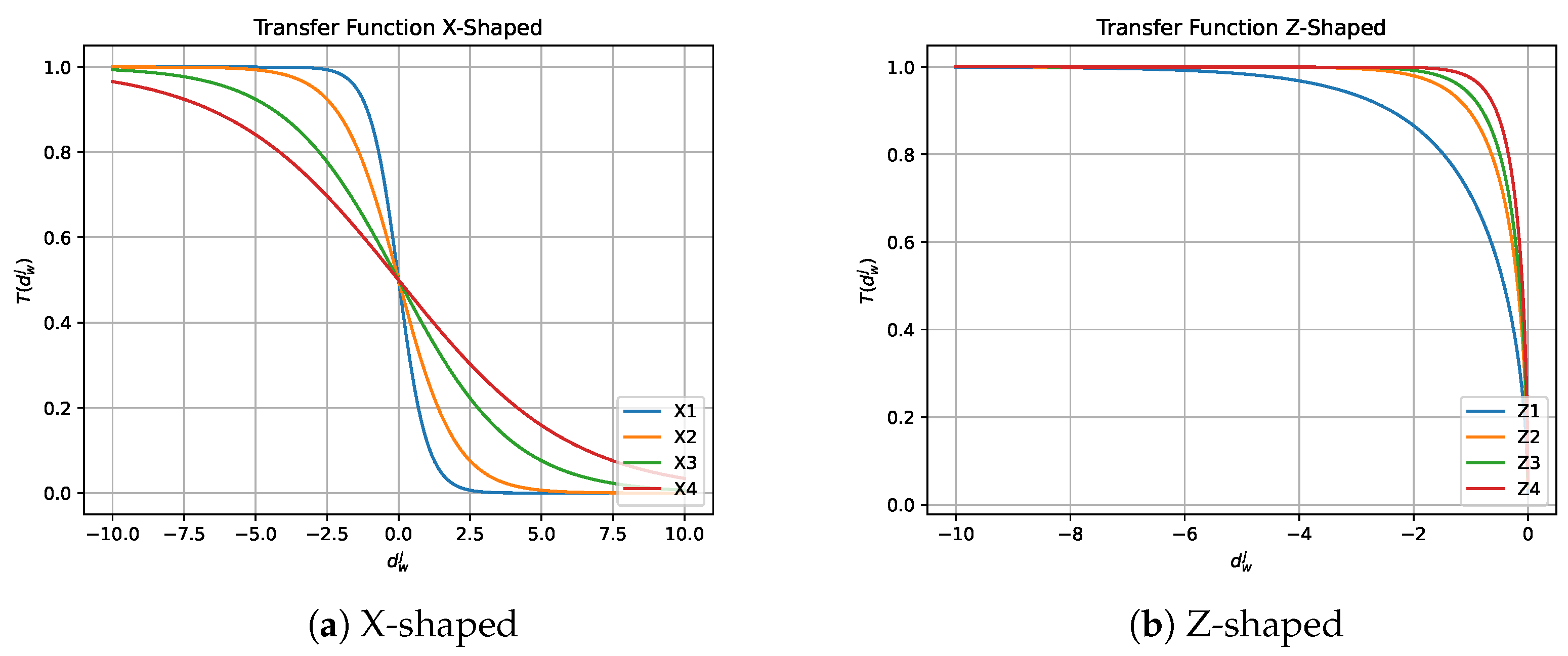
2.2.1. Transfer Function
2.2.2. Binarization Rule
2.3. Metaheuristics
2.3.1. Sine Cosine Algorithm
- is a linearly decreasing parameter and is calculated as follows: , where a is a constant, t is the current iteration, and represents the maximum iterations allowed.This parameter conditions the movement of the solution either towards the best solution () or away from the best solution (). The above equation allows for the balance between exploration and exploitation.
- has values in the range and determines how big the movement of a solution is towards or away from the destination.
- has values in the range and is used to assign a weight to the destination, reinforcing or inhibiting the impact of the destination point on the updating process of the other solutions.
- , with values in the range , is a switch between the sine and cosine functions.
2.3.2. Grey Wolf Optimizer
- Alpha (): these are wolves that are at the top of the hierarchy and lead the pack.
- Beta (): wolves that support the alpha wolves’ decisions.
- Delta (): they are strong but lack leadership skills.
- Omega: they have no power, they are dedicated to follow, help, and protect the younger members of the pack.
2.3.3. Whale Optimization Algorithm
- (1)
- Exploration phase: search for the prey.
- (2)
- Encircling the prey.
- (3)
- Exploitation phase: attacking the prey using a bubble-net method.
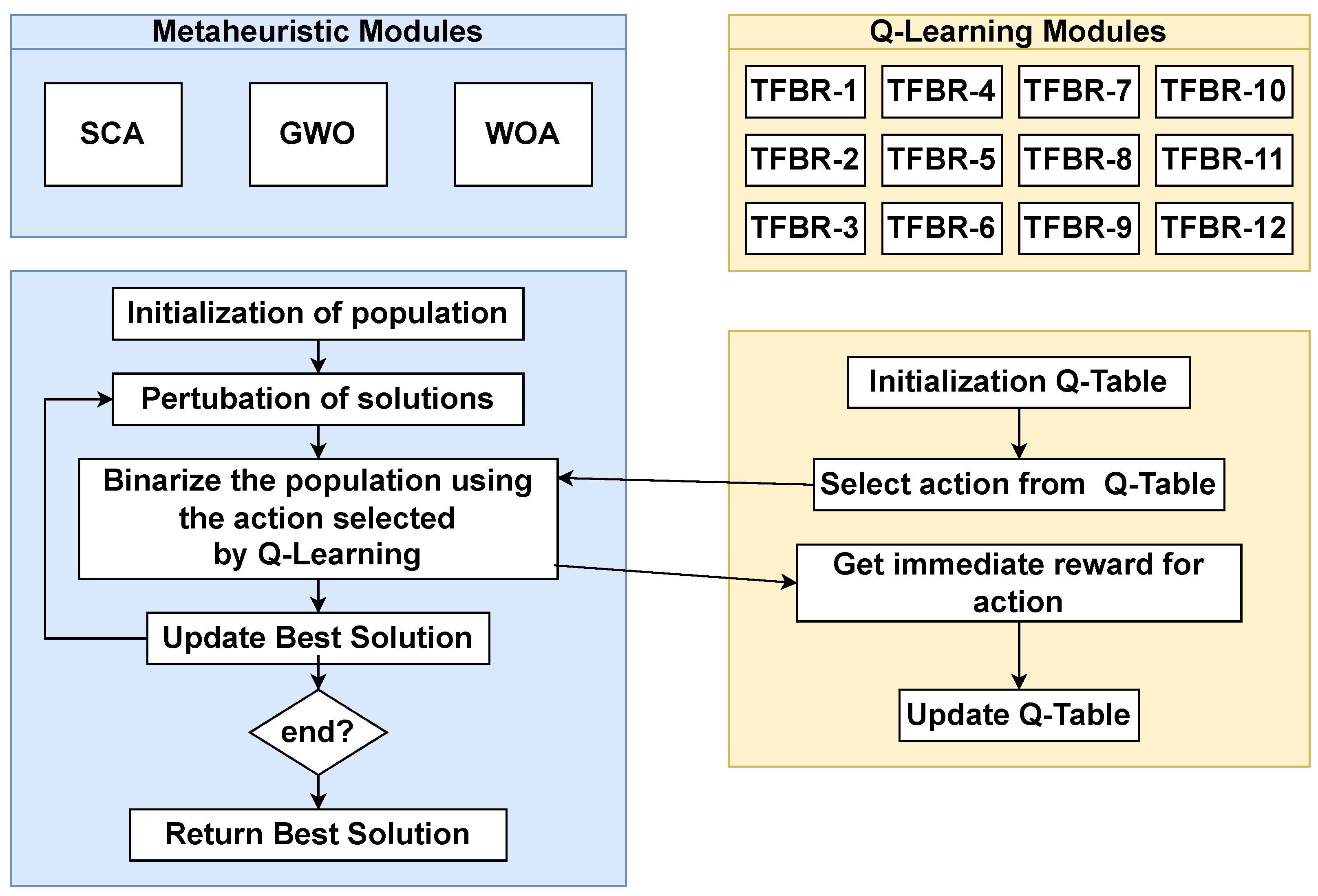
2.4. Hybridization: Binarization Schemes Selector
2.4.1. Actions
2.4.2. States
3. The Proposal: Analysis of Different Sets of Actions
- (1)
- Which will have more impact on binarization, the transfer function or the binarization rule?
- (2)
- Will the binarization schemes selector work better with more actions?
4. Experimental Results
4.1. Set Covering Problem
4.2. Summary of Results
4.2.1. Analysis of the Results Obtained with Grey Wolf Optimizer
4.2.2. Analysis of the Results Obtained with Sine Cosine Algorithm
4.2.3. Analysis of the Results Obtained with Whale Optimization Algorithm
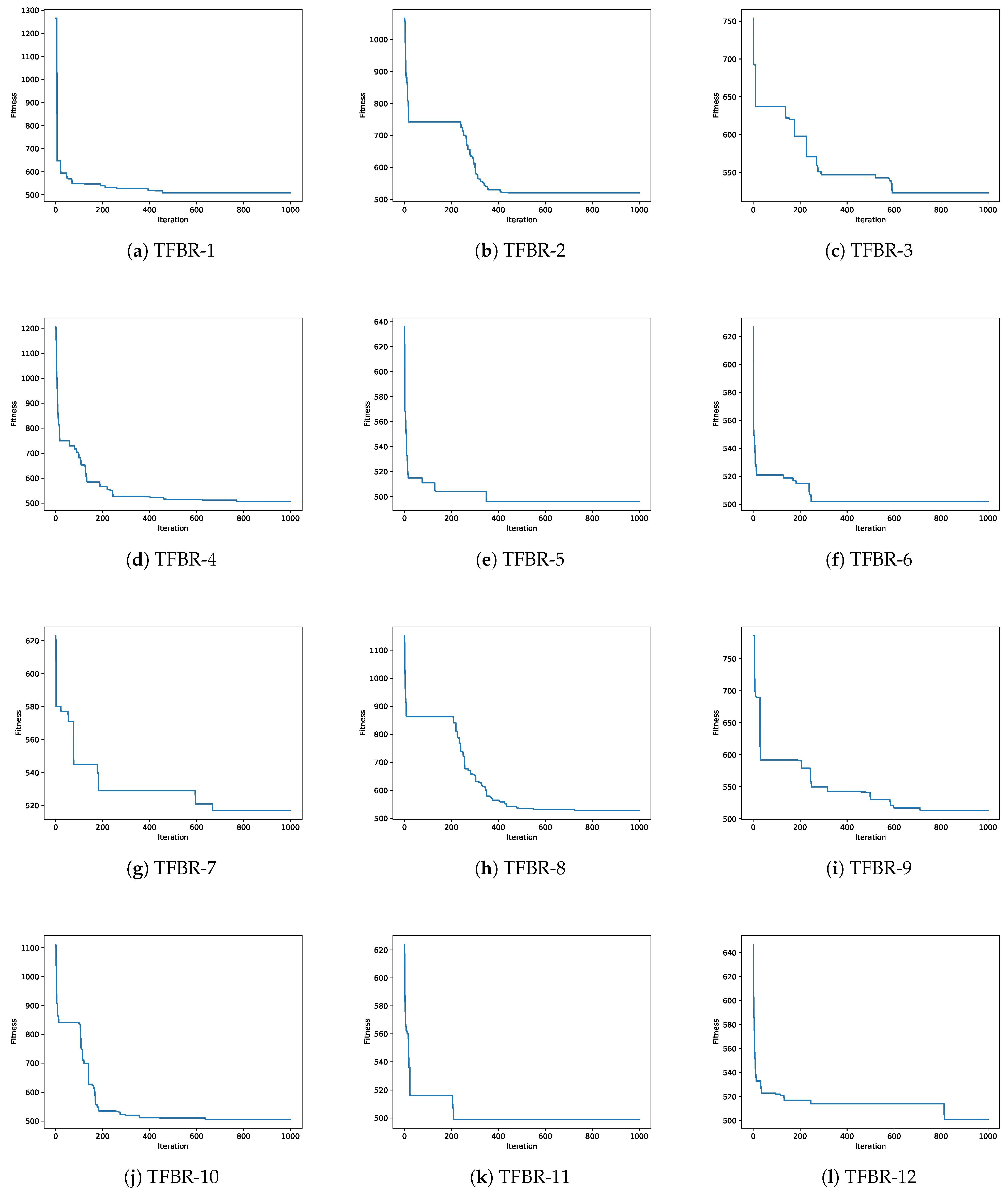
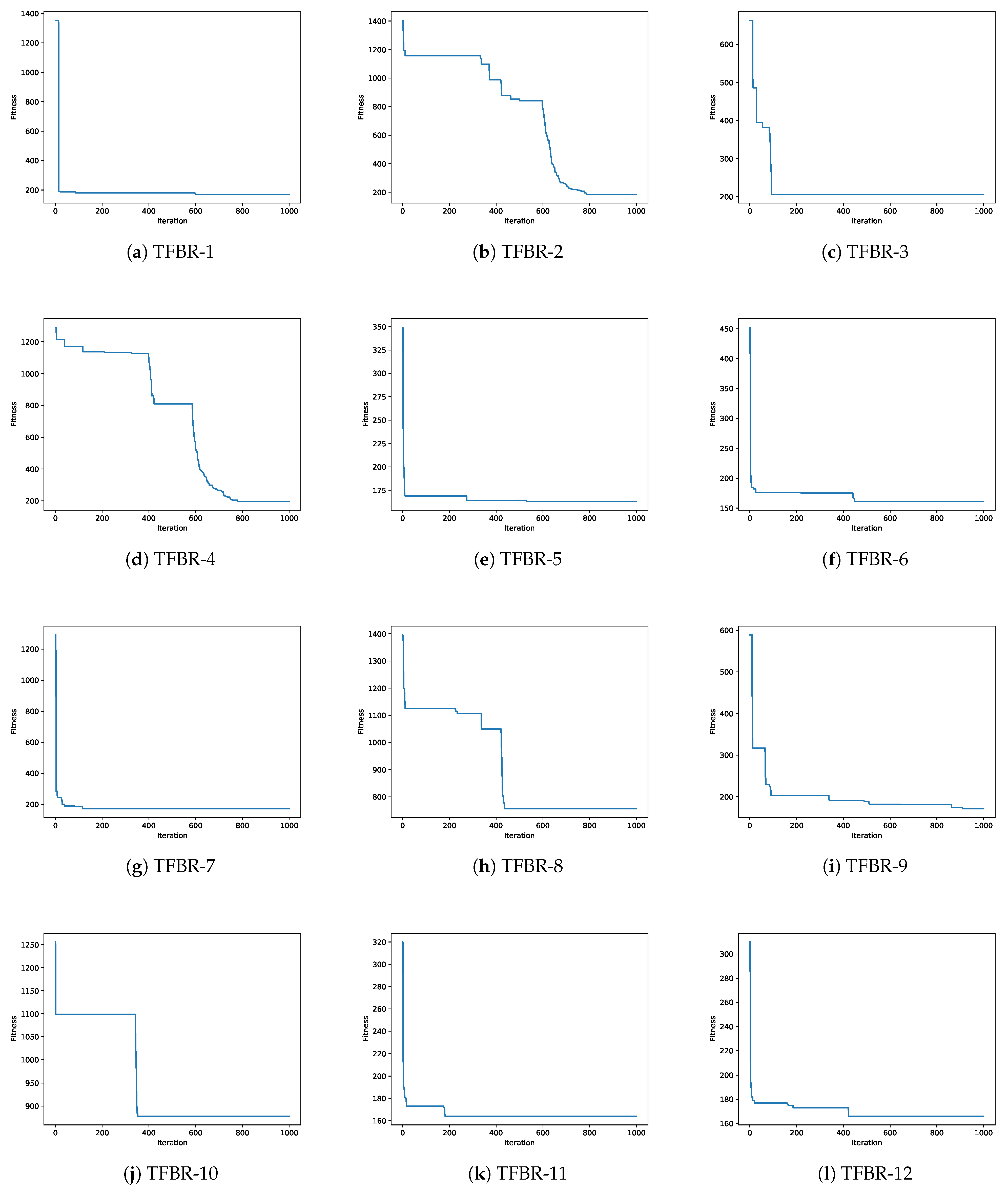
4.3. Convergence Analysis
4.3.1. Analysis of the Convergence Graphs Using Grey Wolf Optimizer

4.3.2. Analysis of the Convergence Graphs Using Sine Cosine Algorithm

4.3.3. Analysis of the Convergence Graphs Using Whale Optimization Algorithm

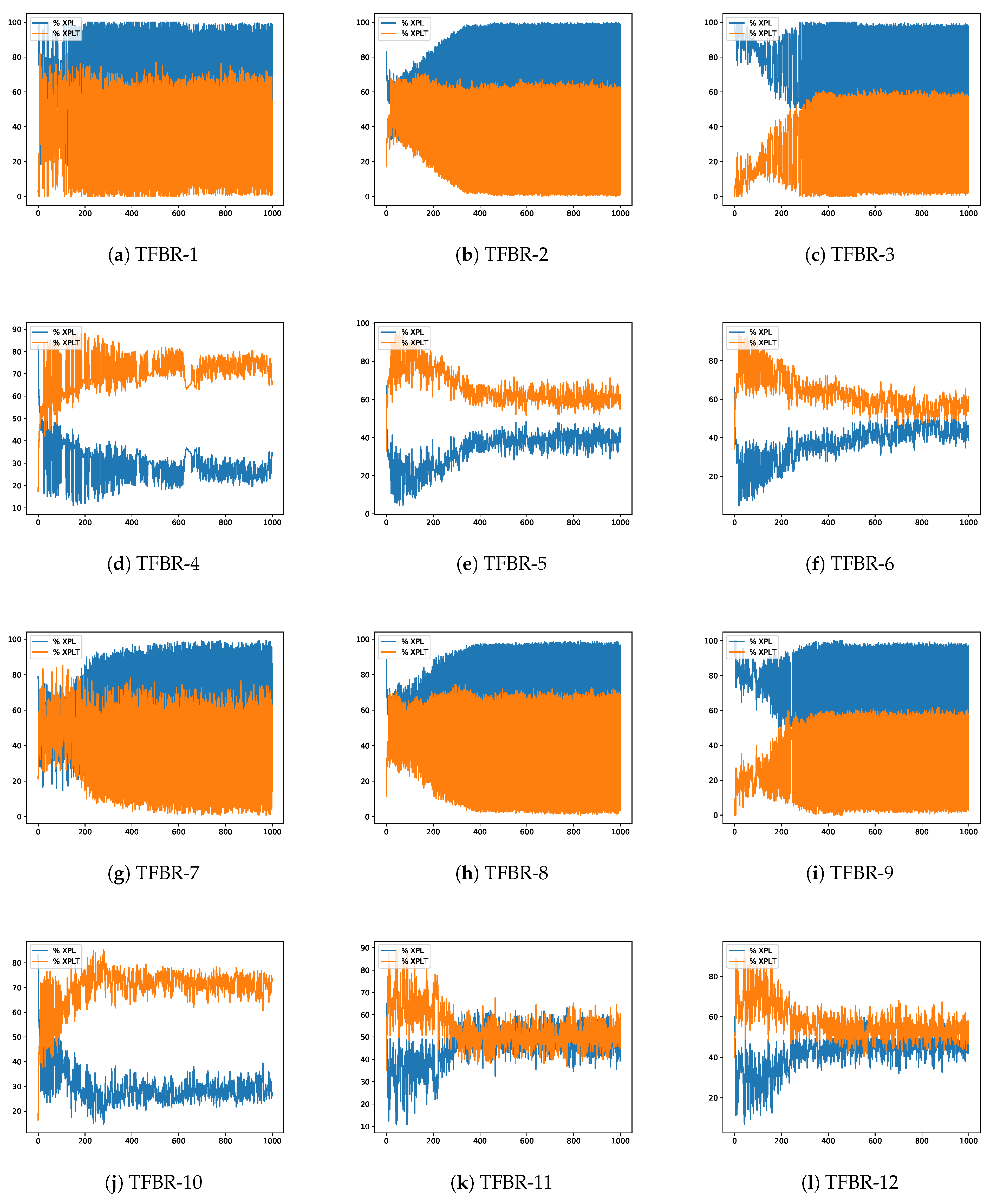
4.4. Exploration and Exploitation Analysis
4.4.1. Analysis of the Percentage Graphs Using Grey Wolf Optimizer
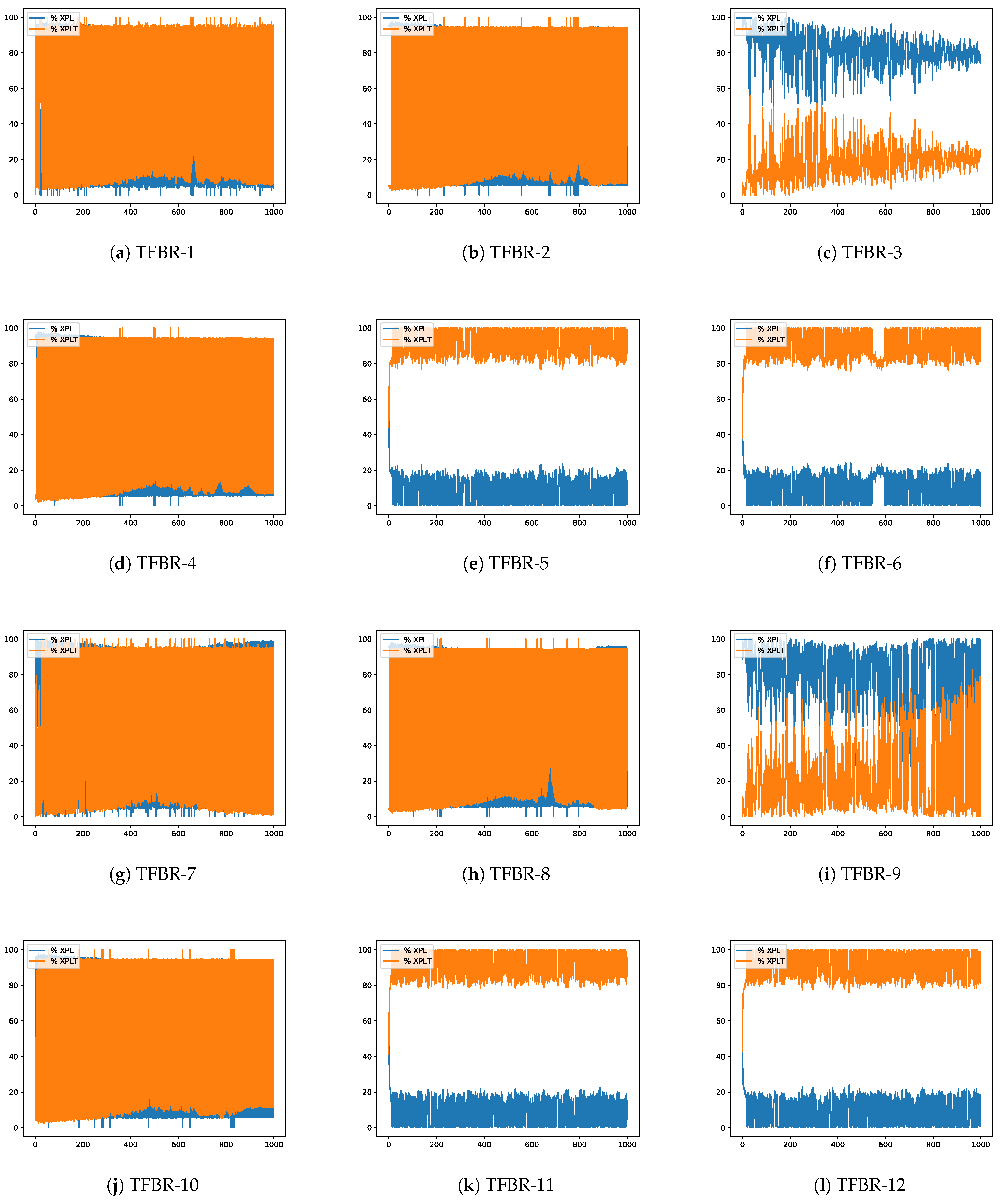
4.4.2. Analysis of the Percentage Graphs Using Sine Cosine Algorithm
4.4.3. Analysis of the Percentage Graphs Using Whale Optimization Algorithm
4.5. Statistical Test
4.6. Summary of the Analysis
- (1)
- Which will have more impact on binarization, the transfer function or the binarization rule?
- (2)
- Will the binarization schemes selector work better with more actions?
5. Conclusions and Outlook
Author Contributions
Funding
Institutional Review Board Statement
Data Availability Statement
Acknowledgments
Conflicts of Interest
References
- Becerra-Rozas, M.; Lemus-Romani, J.; Cisternas-Caneo, F.; Crawford, B.; Soto, R.; Astorga, G.; Castro, C.; García, J. Continuous Metaheuristics for Binary Optimization Problems: An Updated Systematic Literature Review. Mathematics 2022, 11, 129. [Google Scholar]
- Crawford, B.; Soto, R.; Lemus-Romani, J.; Becerra-Rozas, M.; Lanza-Gutiérrez, J.M.; Caballé, N.; Castillo, M.; Tapia, D.; Cisternas-Caneo, F.; García, J.; et al. Q-learnheuristics: Towards data-driven balanced metaheuristics. Mathematics 2021, 9, 1839. [Google Scholar] [CrossRef]
- Ho, Y.; Pepyne, D. Simple explanation of the no-free-lunch theorem and its implications. J. Optim. Theory Appl. 2002, 115, 549–570. [Google Scholar] [CrossRef]
- Mirjalili, S.; Mirjalili, S.M.; Lewis, A. Grey wolf optimizer. Adv. Eng. Softw. 2014, 69, 46–61. [Google Scholar] [CrossRef]
- Mirjalili, S.; Lewis, A. The whale optimization algorithm. Adv. Eng. Softw. 2016, 95, 51–67. [Google Scholar] [CrossRef]
- Mirjalili, S. SCA: A sine cosine algorithm for solving optimization problems. Knowl.-Based Syst. 2016, 96, 120–133. [Google Scholar] [CrossRef]
- Emary, E.; Zawbaa, H.M.; Grosan, C.; Hassenian, A.E. Feature subset selection approach by gray-wolf optimization. In Proceedings of the Afro-European Conference for Industrial Advancement, Villejuif, France, 9–11 September 2015; Springer: Berlin/Heidelberg, Germany, 2015; pp. 1–13. [Google Scholar]
- Kumar, V.; Chhabra, J.K.; Kumar, D. Grey wolf algorithm-based clustering technique. J. Intell. Syst. 2017, 26, 153–168. [Google Scholar] [CrossRef]
- Eswaramoorthy, S.; Sivakumaran, N.; Sekaran, S. Grey wolf optimization based parameter selection for support vector machines. COMPEL-Int. J. Comput. Math. Electr. Electron. Eng. 2016, 35, 1513–1523. [Google Scholar] [CrossRef]
- Li, S.X.; Wang, J.S. Dynamic modeling of steam condenser and design of PI controller based on grey wolf optimizer. Math. Probl. Eng. 2015, 2015, 120975. [Google Scholar] [CrossRef]
- Wong, L.I.; Sulaiman, M.; Mohamed, M.; Hong, M.S. Grey Wolf Optimizer for solving economic dispatch problems. In Proceedings of the 2014 IEEE International Conference on Power and Energy (PECon), Kuching, Malaysia, 1–3 December 2014; pp. 150–154. [Google Scholar]
- Tsai, P.W.; Nguyen, T.-T.; Dao, T.-K. Robot path planning optimization based on multiobjective grey wolf optimizer. In Proceedings of the International Conference on Genetic and Evolutionary Computing, Denver, CO, USA, 20–24 July 2016; Springer: Berlin/Heidelberg, Germany, 2016; pp. 166–173. [Google Scholar]
- Lu, C.; Gao, L.; Li, X.; Xiao, S. A hybrid multi-objective grey wolf optimizer for dynamic scheduling in a real-world welding industry. Eng. Appl. Artif. Intell. 2017, 57, 61–79. [Google Scholar] [CrossRef]
- Mosavi, M.R.; Khishe, M.; Ghamgosar, A. Classification of sonar data set using neural network trained by gray wolf optimization. Neural Netw. World 2016, 26, 393. [Google Scholar] [CrossRef]
- Bentouati, B.; Chaib, L.; Chettih, S. A hybrid whale algorithm and pattern search technique for optimal power flow problem. In Proceedings of the 2016 8th international conference on modelling, identification and control (ICMIC), Algiers, Algeria, 15–17 November 2016; pp. 1048–1053. [Google Scholar]
- Touma, H.J. Study of the economic dispatch problem on IEEE 30-bus system using whale optimization algorithm. Int. J. Eng. Technol. Sci. 2016, 3, 11–18. [Google Scholar] [CrossRef]
- Yin, X.; Cheng, L.; Wang, X.; Lu, J.; Qin, H. Optimization for hydro-photovoltaic-wind power generation system based on modified version of multi-objective whale optimization algorithm. Energy Procedia 2019, 158, 6208–6216. [Google Scholar] [CrossRef]
- Abd El Aziz, M.; Ewees, A.A.; Hassanien, A.E. Whale optimization algorithm and moth-flame optimization for multilevel thresholding image segmentation. Expert Syst. Appl. 2017, 83, 242–256. [Google Scholar] [CrossRef]
- Mafarja, M.M.; Mirjalili, S. Hybrid whale optimization algorithm with simulated annealing for feature selection. Neurocomputing 2017, 260, 302–312. [Google Scholar] [CrossRef]
- Tharwat, A.; Moemen, Y.S.; Hassanien, A.E. Classification of toxicity effects of biotransformed hepatic drugs using whale optimized support vector machines. J. Biomed. Inform. 2017, 68, 132–149. [Google Scholar] [CrossRef]
- Zhao, H.; Guo, S.; Zhao, H. Energy-related CO2 emissions forecasting using an improved LSSVM model optimized by whale optimization algorithm. Energies 2017, 10, 874. [Google Scholar] [CrossRef]
- Banerjee, A.; Nabi, M. Re-entry trajectory optimization for space shuttle using sine-cosine algorithm. In Proceedings of the 2017 8th International Conference on Recent Advances in Space Technologies (RAST), Istanbul, Turkey, 19–22 June 2017; pp. 73–77. [Google Scholar]
- Sindhu, R.; Ngadiran, R.; Yacob, Y.M.; Zahri, N.A.H.; Hariharan, M. Sine–cosine algorithm for feature selection with elitism strategy and new updating mechanism. Neural Comput. Appl. 2017, 28, 2947–2958. [Google Scholar] [CrossRef]
- Mahdad, B.; Srairi, K. A new interactive sine cosine algorithm for loading margin stability improvement under contingency. Electr. Eng. 2018, 100, 913–933. [Google Scholar] [CrossRef]
- Padmanaban, S.; Priyadarshi, N.; Holm-Nielsen, J.B.; Bhaskar, M.S.; Azam, F.; Sharma, A.K.; Hossain, E. A novel modified sine-cosine optimized MPPT algorithm for grid integrated PV system under real operating conditions. IEEE Access 2019, 7, 10467–10477. [Google Scholar] [CrossRef]
- Gonidakis, D.; Vlachos, A. A new sine cosine algorithm for economic and emission dispatch problems with price penalty factors. J. Inf. Optim. Sci. 2019, 40, 679–697. [Google Scholar] [CrossRef]
- Abd Elfattah, M.; Abuelenin, S.; Hassanien, A.E.; Pan, J.S. Handwritten arabic manuscript image binarization using sine cosine optimization algorithm. In Proceedings of the International Conference on Genetic and Evolutionary Computing, Denver, CO, USA, 20–24 July 2016; Springer: Berlin/Heidelberg, Germany, 2016; pp. 273–280. [Google Scholar]
- Mirjalili, S.; Mirjalili, S.M.; Yang, X.S. Binary bat algorithm. Neural Comput. Appl. 2014, 25, 663–681. [Google Scholar] [CrossRef]
- Rodrigues, D.; Pereira, L.A.; Nakamura, R.Y.; Costa, K.A.; Yang, X.S.; Souza, A.N.; Papa, J.P. A wrapper approach for feature selection based on Bat Algorithm and Optimum-Path Forest. Expert Syst. Appl. 2014, 41, 2250–2258. [Google Scholar] [CrossRef]
- Mirjalili, S.; Lewis, A. S-shaped versus V-shaped transfer functions for binary particle swarm optimization. Swarm Evol. Comput. 2013, 9, 1–14. [Google Scholar] [CrossRef]
- Cisternas-Caneo, F.; Crawford, B.; Soto, R.; de la Fuente-Mella, H.; Tapia, D.; Lemus-Romani, J.; Castillo, M.; Becerra-Rozas, M.; Paredes, F.; Misra, S. A Data-Driven Dynamic Discretization Framework to Solve Combinatorial Problems Using Continuous Metaheuristics. In Innovations in Bio-Inspired Computing and Applications; Abraham, A., Sasaki, H., Rios, R., Gandhi, N., Singh, U., Ma, K., Eds.; Springer: Cham, Switzerland, 2021; pp. 76–85. [Google Scholar] [CrossRef]
- Lemus-Romani, J.; Becerra-Rozas, M.; Crawford, B.; Soto, R.; Cisternas-Caneo, F.; Vega, E.; Castillo, M.; Tapia, D.; Astorga, G.; Palma, W.; et al. A Novel Learning-Based Binarization Scheme Selector for Swarm Algorithms Solving Combinatorial Problems. Mathematics 2021, 9, 2887. [Google Scholar] [CrossRef]
- Taghian, S.; Nadimi-Shahraki, M. Binary Sine Cosine Algorithms for Feature Selection from Medical Data. arXiv 2019, arXiv:1911.07805. [Google Scholar] [CrossRef]
- Faris, H.; Mafarja, M.M.; Heidari, A.A.; Aljarah, I.; Ala’M, A.Z.; Mirjalili, S.; Fujita, H. An efficient binary salp swarm algorithm with crossover scheme for feature selection problems. Knowl.-Based Syst. 2018, 154, 43–67. [Google Scholar] [CrossRef]
- Tubishat, M.; Ja’afar, S.; Alswaitti, M.; Mirjalili, S.; Idris, N.; Ismail, M.A.; Omar, M.S. Dynamic Salp swarm algorithm for feature selection. Expert Syst. Appl. 2021, 164, 113873. [Google Scholar] [CrossRef]
- Tapia, D.; Crawford, B.; Soto, R.; Palma, W.; Lemus-Romani, J.; Cisternas-Caneo, F.; Castillo, M.; Becerra-Rozas, M.; Paredes, F.; Misra, S. Embedding Q-Learning in the selection of metaheuristic operators: The enhanced binary grey wolf optimizer case. In Proceedings of the 2021 IEEE International Conference on Automation/XXIV Congress of the Chilean Association of Automatic Control (ICA-ACCA), Valparaiso, Chile, 22–26 March 2021; pp. 1–6. [Google Scholar] [CrossRef]
- Sharma, P.; Sundaram, S.; Sharma, M.; Sharma, A.; Gupta, D. Diagnosis of Parkinson’s disease using modified grey wolf optimization. Cogn. Syst. Res. 2019, 54, 100–115. [Google Scholar] [CrossRef]
- Mafarja, M.; Aljarah, I.; Heidari, A.A.; Faris, H.; Fournier-Viger, P.; Li, X.; Mirjalili, S. Binary dragonfly optimization for feature selection using time-varying transfer functions. Knowl.-Based Syst. 2018, 161, 185–204. [Google Scholar] [CrossRef]
- Eluri, R.K.; Devarakonda, N. Binary Golden Eagle Optimizer with Time-Varying Flight Length for feature selection. Knowl.-Based Syst. 2022, 247, 108771. [Google Scholar] [CrossRef]
- Becerra-Rozas, M.; Lemus-Romani, J.; Crawford, B.; Soto, R.; Cisternas-Caneo, F.; Embry, A.T.; Molina, M.A.; Tapia, D.; Castillo, M.; Misra, S.; et al. Reinforcement Learning Based Whale Optimizer. In Proceedings of the Computational Science and Its Applications—ICCSA 2021, Cagliari, Italy, 13–16 September 2021; Gervasi, O., Murgante, B., Misra, S., Garau, C., Blečić, I., Taniar, D., Apduhan, B.O., Rocha, A.M.A.C., Tarantino, E., Torre, C.M., Eds.; Springer: Cham, Switzerland, 2021; pp. 205–219. [Google Scholar] [CrossRef]
- Mirjalili, S.; Hashim, S.Z.M. BMOA: Binary magnetic optimization algorithm. Int. J. Mach. Learn. Comput. 2012, 2, 204. [Google Scholar] [CrossRef]
- Crawford, B.; Soto, R.; Astorga, G.; García, J.; Castro, C.; Paredes, F. Putting continuous metaheuristics to work in binary search spaces. Complexity 2017, 2017, 8404231. [Google Scholar] [CrossRef]
- Leonard, B.J.; Engelbrecht, A.P.; Cleghorn, C.W. Critical considerations on angle modulated particle swarm optimisers. Swarm Intell. 2015, 9, 291–314. [Google Scholar] [CrossRef]
- Zhang, G. Quantum-inspired evolutionary algorithms: A survey and empirical study. J. Heuristics 2011, 17, 303–351. [Google Scholar] [CrossRef]
- García, J.; Crawford, B.; Soto, R.; Castro, C.; Paredes, F. A k-means binarization framework applied to multidimensional knapsack problem. Appl. Intell. 2018, 48, 357–380. [Google Scholar] [CrossRef]
- García, J.; Moraga, P.; Valenzuela, M.; Crawford, B.; Soto, R.; Pinto, H.; Peña, A.; Altimiras, F.; Astorga, G. A Db-Scan Binarization Algorithm Applied to Matrix Covering Problems. Comput. Intell. Neurosci. 2019, 2019, 3238574. [Google Scholar] [CrossRef]
- Saremi, S.; Mirjalili, S.; Lewis, A. How important is a transfer function in discrete heuristic algorithms. Neural Comput. Appl. 2015, 26, 625–640. [Google Scholar] [CrossRef]
- Kennedy, J.; Eberhart, R.C. A discrete binary version of the particle swarm algorithm. In Proceedings of the 1997 IEEE International Conference on Systems, Man, and Cybernetics. Computational Cybernetics and Simulation, Orlando, FL, USA, 12–15 October 1997; Volume 5, pp. 4104–4108. [Google Scholar] [CrossRef]
- Crawford, B.; Soto, R.; Olivares-Suarez, M.; Palma, W.; Paredes, F.; Olguin, E.; Norero, E. A binary coded firefly algorithm that solves the set covering problem. Rom. J. Inf. Sci. Technol. 2014, 17, 252–264. [Google Scholar]
- Rajalakshmi, N.; Padma Subramanian, D.; Thamizhavel, K. Performance enhancement of radial distributed system with distributed generators by reconfiguration using binary firefly algorithm. J. Inst. Eng. (India) Ser. B 2015, 96, 91–99. [Google Scholar] [CrossRef]
- Ghosh, K.K.; Singh, P.K.; Hong, J.; Geem, Z.W.; Sarkar, R. Binary social mimic optimization algorithm with x-shaped transfer function for feature selection. IEEE Access 2020, 8, 97890–97906. [Google Scholar] [CrossRef]
- Beheshti, Z. A novel x-shaped binary particle swarm optimization. Soft Comput. 2021, 25, 3013–3042. [Google Scholar] [CrossRef]
- Guo, S.s.; Wang, J.s.; Guo, M.w. Z-shaped transfer functions for binary particle swarm optimization algorithm. Comput. Intell. Neurosci. 2020, 2020, 6502807. [Google Scholar] [CrossRef]
- Sun, W.Z.; Zhang, M.; Wang, J.S.; Guo, S.S.; Wang, M.; Hao, W.K. Binary Particle Swarm Optimization Algorithm Based on Z-shaped Probability Transfer Function to Solve 0–1 Knapsack Problem. IAENG Int. J. Comput. Sci. 2021, 48, 2. [Google Scholar]
- Islam, M.J.; Li, X.; Mei, Y. A time-varying transfer function for balancing the exploration and exploitation ability of a binary PSO. Appl. Soft Comput. 2017, 59, 182–196. [Google Scholar] [CrossRef]
- Mohd Yusof, N.; Muda, A.K.; Pratama, S.F.; Carbo-Dorca, R.; Abraham, A. Improved swarm intelligence algorithms with time-varying modified Sigmoid transfer function for Amphetamine-type stimulants drug classification. Chemom. Intell. Lab. Syst. 2022, 226, 104574. [Google Scholar] [CrossRef]
- Mohd Yusof, N.; Muda, A.K.; Pratama, S.F.; Abraham, A. A novel nonlinear time-varying sigmoid transfer function in binary whale optimization algorithm for descriptors selection in drug classification. Mol. Divers. 2022, 27, 71–80. [Google Scholar] [CrossRef]
- Lanza-Gutierrez, J.M.; Crawford, B.; Soto, R.; Berrios, N.; Gomez-Pulido, J.A.; Paredes, F. Analyzing the effects of binarization techniques when solving the set covering problem through swarm optimization. Expert Syst. Appl. 2017, 70, 67–82. [Google Scholar] [CrossRef]
- Talbi, E.G. Metaheuristics: From Design to Implementation; John Wiley & Sons: Hoboken, NJ, USA, 2009. [Google Scholar]
- Becerra-Rozas, M.; Lemus-Romani, J.; Cisternas-Caneo, F.; Crawford, B.; Soto, R.; García, J. Swarm-Inspired Computing to Solve Binary Optimization Problems: A Backward Q-Learning Binarization Scheme Selector. Mathematics 2022, 10, 4776. [Google Scholar] [CrossRef]
- Becerra-Rozas, M.; Cisternas-Caneo, F.; Crawford, B.; Soto, R.; García, J.; Astorga, G.; Palma, W. Embedded Learning Approaches in the Whale Optimizer to Solve Coverage Combinatorial Problems. Mathematics 2022, 10, 4529. [Google Scholar] [CrossRef]
- Hussain, K.; Zhu, W.; Mohd Salleh, M.N. Long-Term Memory Harris’ Hawk Optimization for High Dimensional and Optimal Power Flow Problems. IEEE Access 2019, 7, 147596–147616. [Google Scholar] [CrossRef]
- Morales-Castañeda, B.; Zaldívar, D.; Cuevas, E.; Fausto, F.; Rodríguez, A. A better balance in metaheuristic algorithms: Does it exist? Swarm Evol. Comput. 2020, 54, 100671. [Google Scholar] [CrossRef]
- Beasley, J.; Jørnsten, K. Enhancing an algorithm for set covering problems. Eur. J. Oper. Res. 1992, 58, 293–300. [Google Scholar] [CrossRef]
- Bisong, E. Google Colaboratory. In Building Machine Learning and Deep Learning Models on Google Cloud Platform: A Comprehensive Guide for Beginners; Apress: Berkeley, CA, USA, 2019; pp. 59–64. [Google Scholar] [CrossRef]
- Garey, M.R.; Johnson, D.S. Computers and Intractability: A Guide to the Theory of NP-completeness. J. Symb. Log. 1979, 48, 498–500. [Google Scholar] [CrossRef]
- Lanza-Gutierrez, J.M.; Caballe, N.; Crawford, B.; Soto, R.; Gomez-Pulido, J.A.; Paredes, F. Exploring Further Advantages in an Alternative Formulation for the Set Covering Problem. Math. Probl. Eng. 2020, 2020, 5473501. [Google Scholar] [CrossRef]
- Smith, B.M. IMPACS-a bus crew scheduling system using integer programming. Math. Program. 1988, 42, 181–187. [Google Scholar] [CrossRef]
- Vianna, S.S. The set covering problem applied to optimisation of gas detectors in chemical process plants. Comput. Chem. Eng. 2019, 121, 388–395. [Google Scholar] [CrossRef]
- Liu, Z.; Xu, H.; Liu, P.; Li, L.; Zhao, X. Interval-valued intuitionistic uncertain linguistic multi-attribute decision-making method for plant location selection with partitioned hamy mean. Int. J. Fuzzy Syst. 2020, 22, 1993–2010. [Google Scholar] [CrossRef]
- Bahrami, I.; Ahari, R.M.; Asadpour, M. A maximal covering facility location model for emergency services within an M (t)/M/m/m queuing system. J. Model. Manag. 2020, 16, 963–986. [Google Scholar] [CrossRef]
- Xiang, X.; Qiu, J.; Xiao, J.; Zhang, X. Demand coverage diversity based ant colony optimization for dynamic vehicle routing problems. Eng. Appl. Artif. Intell. 2020, 91, 103582. [Google Scholar] [CrossRef]
- Zhang, L.; Shaffer, B.; Brown, T.; Scott Samuelsen, G. The optimization of DC fast charging deployment in California. Appl. Energy 2015, 157, 111–122. [Google Scholar] [CrossRef]
- Mandal, S.; Patra, N.; Pal, M. Covering problem on fuzzy graphs and its application in disaster management system. Soft Comput. 2021, 25, 2545–2557. [Google Scholar] [CrossRef]
- Alizadeh, R.; Nishi, T. Hybrid Set Covering and Dynamic Modular Covering Location Problem: Application to an Emergency Humanitarian Logistics Problem. Appl. Sci. 2020, 10, 7110. [Google Scholar] [CrossRef]
- Park, Y.; Nielsen, P.; Moon, I. Unmanned aerial vehicle set covering problem considering fixed-radius coverage constraint. Comput. Oper. Res. 2020, 119, 104936. [Google Scholar] [CrossRef]
- Mann, H.B.; Whitney, D.R. On a test of whether one of two random variables is stochastically larger than the other. Ann. Math. Stat. 1947, 18, 50–60. [Google Scholar] [CrossRef]


| Transfer Functions | |||
|---|---|---|---|
| S-shaped [30,49] | V-shaped [30,49,50] | ||
| Name | Equation | Name | Equation |
| S1 | V1 | ||
| S2 | V2 | ||
| S3 | V3 | ||
| S4 | V4 | ||
| Transfer Functions | |||
|---|---|---|---|
| X-shaped [51,52] | Z-shaped [53,54] | ||
| Name | Equation | Name | Equation |
| X1 | Z1 | ||
| X2 | Z2 | ||
| X3 | Z3 | ||
| X4 | Z4 | ||
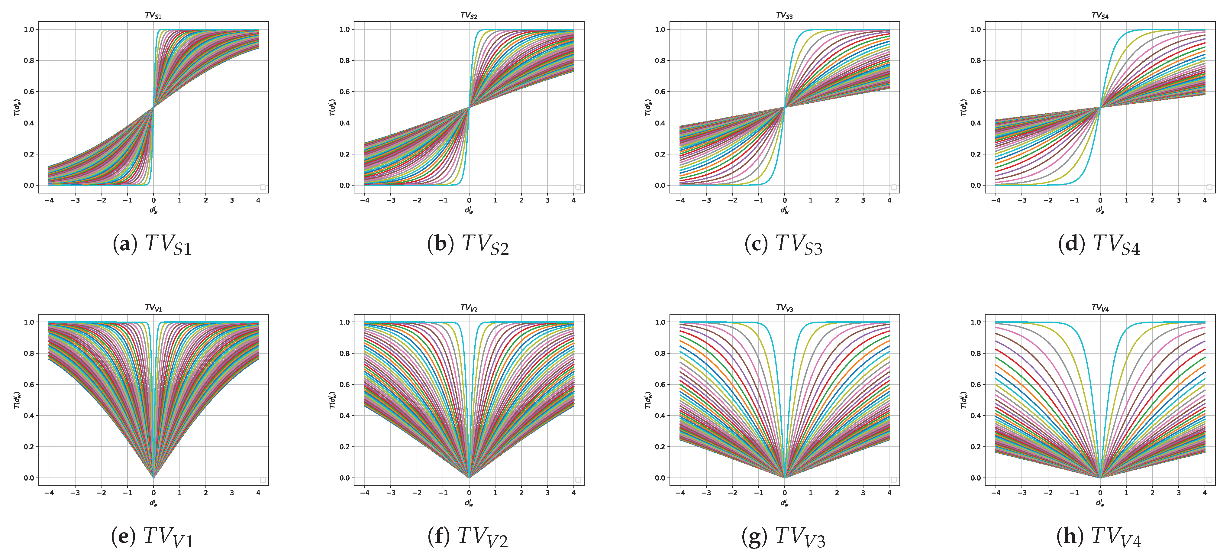
| Time-Varying Transfer Functions [38] | |||
|---|---|---|---|
| S-shaped | V-shaped | ||
| Name | Equation | Name | Equation |
| Type | Binarization Rules |
|---|---|
| Standard | |
| Complement | |
| Static Probability | |
| Elitist | |
| Roulette Elitist |
| Set of Actions | |||
|---|---|---|---|
| Set ID | Transfer Functions | Binarization Rules | Amount of actions |
| TFBR-1 | S-shaped and V-shaped | Standard, Complement, Static Probability, Elitist, and Roulette Elitist | 40 |
| TFBR-2 | S-shaped and V-shaped | Standard | 8 |
| TFBR-3 | S-shaped and V-shaped | Complement | 8 |
| TFBR-4 | S-shaped and V-shaped | Static Probability | 8 |
| TFBR-5 | S-shaped and V-shaped | Elitist | 8 |
| TFBR-6 | S-shaped and V-shaped | Roulette Elitist | 8 |
| TFBR-7 | S-shaped, V-shaped, X-shaped and Z-shaped | Standard, Complement, Static Probability, Elitist, and Roulette Elitist | 80 |
| TFBR-8 | S-shaped, V-shaped, X-shaped, and Z-shaped | Standard | 16 |
| TFBR-9 | S-shaped, V-shaped, X-shaped, and Z-shaped | Complement | 16 |
| TFBR-10 | S-shaped, V-shaped, X-shaped, and Z-shaped | Static Probability | 16 |
| TFBR-11 | S-shaped, V-shaped, X-shaped, and Z-shaped | Elitist | 16 |
| TFBR-12 | S-shaped, V-shaped, X-shaped, and Z-shaped | Roulette Elitist | 16 |
| Parameter | Value |
|---|---|
| Independent runs | 31 |
| Number of populations | 40 |
| Number of iterations | 1000 |
| Parameter a of SCA | 2 |
| Parameter a of GWO | Decreases linearly from 2 to 0 |
| Parameter a of WOA | Decreases linearly from 2 to 0 |
| Parameter b of WOA | 1 |
| Parameter of Q-learning | 0.1 |
| Parameter of Q-learning | 0.4 |
| RPD | TFBR-1 | TFBR-2 | TFBR-3 | TFBR-4 | TFBR-5 | TFBR-6 | TFBR-7 | TFBR-8 | TFBR-9 | TFBR-10 | TFBR-11 | TFBR-12 |
|---|---|---|---|---|---|---|---|---|---|---|---|---|
| 0 | 0 | 0 | 0 | 0 | 12 | 8 | 0 | 0 | 0 | 1 | 8 | 8 |
| 20 | 1 | 1 | 13 | 30 | 32 | 13 | 1 | 7 | 25 | 33 | 33 | |
| 11 | 3 | 6 | 10 | 3 | 5 | 17 | 2 | 11 | 8 | 4 | 4 | |
| >5 | 14 | 41 | 38 | 22 | 0 | 0 | 15 | 42 | 27 | 11 | 0 | 0 |
| RPD | TFBR-1 | TFBR-2 | TFBR-3 | TFBR-4 | TFBR-5 | TFBR-6 | TFBR-7 | TFBR-8 | TFBR-9 | TFBR-10 | TFBR-11 | TFBR-12 |
|---|---|---|---|---|---|---|---|---|---|---|---|---|
| 0 | 0 | 0 | 0 | 0 | 6 | 7 | 1 | 0 | 0 | 0 | 6 | 6 |
| 13 | 0 | 9 | 0 | 33 | 33 | 14 | 0 | 14 | 0 | 31 | 33 | |
| 16 | 0 | 1 | 0 | 5 | 4 | 21 | 0 | 10 | 0 | 7 | 5 | |
| >5 | 16 | 45 | 44 | 45 | 1 | 1 | 9 | 45 | 21 | 45 | 1 | 1 |
| RPD | TFBR-1 | TFBR-2 | TFBR-3 | TFBR-4 | TFBR-5 | TFBR-6 | TFBR-7 | TFBR-8 | TFBR-9 | TFBR-10 | TFBR-11 | TFBR-12 |
|---|---|---|---|---|---|---|---|---|---|---|---|---|
| 0 | 1 | 0 | 0 | 0 | 8 | 10 | 0 | 0 | 1 | 0 | 6 | 7 |
| 18 | 4 | 0 | 1 | 32 | 29 | 22 | 0 | 21 | 0 | 31 | 27 | |
| 18 | 1 | 1 | 3 | 5 | 6 | 15 | 0 | 15 | 0 | 7 | 11 | |
| >5 | 8 | 40 | 44 | 41 | 0 | 0 | 8 | 45 | 8 | 45 | 1 | 0 |
| SCP | TFBR-1 | TFBR-2 | TFBR-3 | TFBR-4 | TFBR-5 | TFBR-6 | |||||||||||||
|---|---|---|---|---|---|---|---|---|---|---|---|---|---|---|---|---|---|---|---|
| Inst. | Opt. | Best | Avg | RPD | Best | Avg | RPD | Best | Avg | RPD | Best | Avg | RPD | Best | Avg | RPD | Best | Avg | RPD |
| 41 | 429 | 431.0 | 436.81 | 0.47 | 439.0 | 472.35 | 2.33 | 435.0 | 448.48 | 1.4 | 432.0 | 445.48 | 0.7 | 430.0 | 433.23 | 0.23 | 430.0 | 434.29 | 0.23 |
| 42 | 512 | 532.0 | 543.48 | 3.91 | 562.0 | 611.42 | 9.77 | 551.0 | 578.97 | 7.62 | 543.0 | 558.97 | 6.05 | 521.0 | 530.32 | 1.76 | 518.0 | 529.39 | 1.17 |
| 43 | 516 | 535.0 | 542.71 | 3.68 | 567.0 | 626.97 | 9.88 | 543.0 | 577.71 | 5.23 | 532.0 | 551.94 | 3.1 | 517.0 | 525.68 | 0.19 | 522.0 | 526.1 | 1.16 |
| 44 | 494 | 508.0 | 521.29 | 2.83 | 520.0 | 581.87 | 5.26 | 523.0 | 539.68 | 5.87 | 506.0 | 530.13 | 2.43 | 496.0 | 507.39 | 0.4 | 502.0 | 509.29 | 1.62 |
| 45 | 512 | 532.0 | 545.23 | 3.91 | 547.0 | 602.03 | 6.84 | 552.0 | 581.77 | 7.81 | 529.0 | 552.0 | 3.32 | 520.0 | 526.42 | 1.56 | 521.0 | 527.29 | 1.76 |
| 46 | 560 | 576.0 | 582.39 | 2.86 | 592.0 | 670.77 | 5.71 | 582.0 | 617.52 | 3.93 | 574.0 | 591.94 | 2.5 | 566.0 | 570.26 | 1.07 | 563.0 | 570.29 | 0.54 |
| 47 | 430 | 437.0 | 444.19 | 1.63 | 454.0 | 492.52 | 5.58 | 449.0 | 468.06 | 4.42 | 441.0 | 451.81 | 2.56 | 434.0 | 436.87 | 0.93 | 433.0 | 436.9 | 0.7 |
| 48 | 492 | 502.0 | 508.45 | 2.03 | 510.0 | 598.45 | 3.66 | 522.0 | 547.52 | 6.1 | 506.0 | 524.29 | 2.85 | 494.0 | 500.45 | 0.41 | 493.0 | 500.29 | 0.2 |
| 49 | 641 | 670.0 | 688.58 | 4.52 | 684.0 | 763.71 | 6.71 | 679.0 | 727.52 | 5.93 | 685.0 | 705.81 | 6.86 | 652.0 | 669.13 | 1.72 | 661.0 | 671.68 | 3.12 |
| 410 | 514 | 524.0 | 529.71 | 1.95 | 552.0 | 601.65 | 7.39 | 541.0 | 557.55 | 5.25 | 522.0 | 545.68 | 1.56 | 518.0 | 522.48 | 0.78 | 519.0 | 523.13 | 0.97 |
| 51 | 253 | 261.0 | 266.87 | 3.16 | 277.0 | 305.16 | 9.49 | 264.0 | 283.9 | 4.35 | 263.0 | 272.87 | 3.95 | 257.0 | 261.19 | 1.58 | 255.0 | 262.55 | 0.79 |
| 52 | 302 | 324.0 | 331.48 | 7.28 | 349.0 | 381.45 | 15.56 | 332.0 | 353.74 | 9.93 | 333.0 | 341.32 | 10.26 | 315.0 | 322.9 | 4.3 | 316.0 | 322.45 | 4.64 |
| 53 | 226 | 231.0 | 234.06 | 2.21 | 245.0 | 270.29 | 8.41 | 236.0 | 247.52 | 4.42 | 233.0 | 239.81 | 3.1 | 228.0 | 230.23 | 0.88 | 229.0 | 230.94 | 1.33 |
| 54 | 242 | 249.0 | 252.52 | 2.89 | 254.0 | 283.29 | 4.96 | 255.0 | 265.77 | 5.37 | 252.0 | 260.06 | 4.13 | 244.0 | 248.0 | 0.83 | 245.0 | 248.29 | 1.24 |
| 55 | 211 | 215.0 | 218.26 | 1.9 | 221.0 | 245.84 | 4.74 | 220.0 | 228.55 | 4.27 | 216.0 | 224.74 | 2.37 | 212.0 | 214.55 | 0.47 | 212.0 | 215.48 | 0.47 |
| 56 | 213 | 218.0 | 227.45 | 2.35 | 240.0 | 267.87 | 12.68 | 221.0 | 243.68 | 3.76 | 224.0 | 233.71 | 5.16 | 214.0 | 219.06 | 0.47 | 215.0 | 220.52 | 0.94 |
| 57 | 293 | 307.0 | 312.03 | 4.78 | 320.0 | 354.61 | 9.22 | 317.0 | 333.13 | 8.19 | 308.0 | 318.97 | 5.12 | 298.0 | 303.03 | 1.71 | 297.0 | 303.0 | 1.37 |
| 58 | 288 | 294.0 | 298.42 | 2.08 | 314.0 | 338.06 | 9.03 | 303.0 | 319.06 | 5.21 | 295.0 | 308.77 | 2.43 | 290.0 | 293.9 | 0.69 | 291.0 | 294.52 | 1.04 |
| 59 | 279 | 285.0 | 289.68 | 2.15 | 301.0 | 330.13 | 7.89 | 293.0 | 307.87 | 5.02 | 287.0 | 297.84 | 2.87 | 281.0 | 284.55 | 0.72 | 280.0 | 284.03 | 0.36 |
| 510 | 265 | 274.0 | 278.42 | 3.4 | 292.0 | 318.77 | 10.19 | 284.0 | 296.42 | 7.17 | 274.0 | 283.87 | 3.4 | 268.0 | 272.06 | 1.13 | 266.0 | 271.16 | 0.38 |
| 61 | 138 | 144.0 | 146.58 | 4.35 | 155.0 | 219.35 | 12.32 | 150.0 | 169.94 | 8.7 | 146.0 | 150.87 | 5.8 | 141.0 | 143.23 | 2.17 | 140.0 | 143.06 | 1.45 |
| 62 | 146 | 153.0 | 156.39 | 4.79 | 171.0 | 264.4 | 17.12 | 166.0 | 199.29 | 13.7 | 151.0 | 160.61 | 3.42 | 148.0 | 150.0 | 1.37 | 146.0 | 150.58 | 0.0 |
| 63 | 145 | 147.0 | 150.32 | 1.38 | 189.0 | 250.65 | 30.34 | 152.0 | 184.58 | 4.83 | 149.0 | 155.74 | 2.76 | 145.0 | 148.06 | 0.0 | 147.0 | 148.42 | 1.38 |
| 64 | 131 | 133.0 | 135.0 | 1.53 | 147.0 | 199.0 | 12.21 | 138.0 | 151.16 | 5.34 | 134.0 | 138.45 | 2.29 | 131.0 | 132.77 | 0.0 | 131.0 | 132.9 | 0.0 |
| 65 | 161 | 173.0 | 178.61 | 7.45 | 188.0 | 271.29 | 16.77 | 188.0 | 215.16 | 16.77 | 173.0 | 180.42 | 7.45 | 161.0 | 168.35 | 0.0 | 162.0 | 169.0 | 0.62 |
| a1 | 253 | 262.0 | 268.1 | 3.56 | 309.0 | 362.26 | 22.13 | 286.0 | 314.61 | 13.04 | 270.0 | 278.74 | 6.72 | 258.0 | 262.32 | 1.98 | 259.0 | 262.52 | 2.37 |
| a2 | 252 | 266.0 | 271.81 | 5.56 | 316.0 | 364.42 | 25.4 | 285.0 | 314.1 | 13.1 | 271.0 | 280.77 | 7.54 | 258.0 | 263.61 | 2.38 | 259.0 | 265.29 | 2.78 |
| a3 | 232 | 245.0 | 248.03 | 5.6 | 280.0 | 326.13 | 20.69 | 264.0 | 286.65 | 13.79 | 248.0 | 255.06 | 6.9 | 239.0 | 242.81 | 3.02 | 240.0 | 243.68 | 3.45 |
| a4 | 234 | 247.0 | 251.26 | 5.56 | 273.0 | 332.42 | 16.67 | 269.0 | 295.65 | 14.96 | 247.0 | 262.19 | 5.56 | 236.0 | 242.52 | 0.85 | 236.0 | 242.87 | 0.85 |
| a5 | 236 | 245.0 | 249.77 | 3.81 | 265.0 | 330.97 | 12.29 | 265.0 | 294.39 | 12.29 | 247.0 | 259.87 | 4.66 | 239.0 | 243.42 | 1.27 | 240.0 | 243.61 | 1.69 |
| b1 | 69 | 71.0 | 72.58 | 2.9 | 137.0 | 211.19 | 98.55 | 106.0 | 132.29 | 53.62 | 71.0 | 76.94 | 2.9 | 69.0 | 70.29 | 0.0 | 69.0 | 70.06 | 0.0 |
| b2 | 76 | 78.0 | 80.97 | 2.63 | 146.0 | 196.16 | 92.11 | 112.0 | 142.26 | 47.37 | 81.0 | 86.55 | 6.58 | 76.0 | 77.32 | 0.0 | 76.0 | 77.48 | 0.0 |
| b3 | 80 | 82.0 | 84.13 | 2.5 | 161.0 | 240.94 | 101.25 | 129.0 | 166.84 | 61.25 | 84.0 | 90.13 | 5.0 | 80.0 | 81.06 | 0.0 | 81.0 | 81.45 | 1.25 |
| b4 | 79 | 83.0 | 85.29 | 5.06 | 158.0 | 214.74 | 100.0 | 114.0 | 153.9 | 44.3 | 84.0 | 89.58 | 6.33 | 79.0 | 81.26 | 0.0 | 80.0 | 81.61 | 1.27 |
| b5 | 72 | 73.0 | 75.0 | 1.39 | 140.0 | 193.06 | 94.44 | 101.0 | 137.39 | 40.28 | 73.0 | 82.68 | 1.39 | 72.0 | 72.87 | 0.0 | 72.0 | 72.81 | 0.0 |
| c1 | 227 | 245.0 | 250.68 | 7.93 | 289.0 | 371.32 | 27.31 | 279.0 | 316.45 | 22.91 | 248.0 | 260.52 | 9.25 | 231.0 | 238.45 | 1.76 | 233.0 | 239.1 | 2.64 |
| c2 | 219 | 232.0 | 241.48 | 5.94 | 295.0 | 364.77 | 34.7 | 268.0 | 305.77 | 22.37 | 239.0 | 252.68 | 9.13 | 226.0 | 230.23 | 3.2 | 227.0 | 231.32 | 3.65 |
| c3 | 243 | 256.0 | 263.97 | 5.35 | 348.0 | 415.35 | 43.21 | 293.0 | 343.03 | 20.58 | 267.0 | 280.74 | 9.88 | 248.0 | 252.65 | 2.06 | 248.0 | 253.65 | 2.06 |
| c4 | 219 | 232.0 | 237.06 | 5.94 | 314.0 | 359.52 | 43.38 | 270.0 | 303.9 | 23.29 | 233.0 | 247.97 | 6.39 | 225.0 | 230.9 | 2.74 | 226.0 | 230.52 | 3.2 |
| c5 | 215 | 229.0 | 233.35 | 6.51 | 293.0 | 358.71 | 36.28 | 270.0 | 303.42 | 25.58 | 228.0 | 243.84 | 6.05 | 220.0 | 224.16 | 2.33 | 220.0 | 224.16 | 2.33 |
| d1 | 60 | 65.0 | 66.94 | 8.33 | 171.0 | 250.42 | 185.0 | 130.0 | 174.23 | 116.67 | 66.0 | 72.77 | 10.0 | 60.0 | 61.61 | 0.0 | 61.0 | 62.03 | 1.67 |
| d2 | 66 | 67.0 | 70.9 | 1.52 | 222.0 | 305.71 | 236.36 | 136.0 | 176.35 | 106.06 | 70.0 | 81.03 | 6.06 | 66.0 | 67.45 | 0.0 | 66.0 | 67.87 | 0.0 |
| d3 | 72 | 77.0 | 79.97 | 6.94 | 230.0 | 314.58 | 219.44 | 159.0 | 209.1 | 120.83 | 82.0 | 90.35 | 13.89 | 73.0 | 74.71 | 1.39 | 73.0 | 75.23 | 1.39 |
| d4 | 62 | 63.0 | 65.35 | 1.61 | 155.0 | 254.77 | 150.0 | 125.0 | 163.23 | 101.61 | 65.0 | 75.32 | 4.84 | 62.0 | 62.9 | 0.0 | 62.0 | 62.97 | 0.0 |
| d5 | 61 | 65.0 | 66.74 | 6.56 | 159.0 | 250.29 | 160.66 | 139.0 | 170.06 | 127.87 | 66.0 | 75.13 | 8.2 | 61.0 | 62.35 | 0.0 | 61.0 | 62.68 | 0.0 |
| 263.07 | 268.5 | 3.88 | 305.58 | 363.1 | 43.64 | 286.58 | 314.4 | 25.83 | 265.51 | 277.09 | 5.19 | 256.87 | 261.27 | 1.07 | 257.4 | 261.7 | 1.29 | ||
| SCP | TFBR-7 | TFBR-8 | TFBR-9 | TFBR-10 | TFBR-11 | TFBR-12 | |||||||||||||
|---|---|---|---|---|---|---|---|---|---|---|---|---|---|---|---|---|---|---|---|
| Inst. | Opt. | Best | Avg | RPD | Best | Avg | RPD | Best | Avg | RPD | Best | Avg | RPD | Best | Avg | RPD | Best | Avg | RPD |
| 41 | 429 | 433.0 | 437.87 | 0.93 | 438.0 | 460.39 | 2.1 | 432.0 | 442.55 | 0.7 | 430.0 | 436.06 | 0.23 | 431.0 | 433.39 | 0.47 | 430.0 | 433.52 | 0.23 |
| 42 | 512 | 530.0 | 545.26 | 3.52 | 544.0 | 590.26 | 6.25 | 538.0 | 557.19 | 5.08 | 521.0 | 546.65 | 1.76 | 518.0 | 530.77 | 1.17 | 524.0 | 533.03 | 2.34 |
| 43 | 516 | 533.0 | 544.26 | 3.29 | 554.0 | 598.42 | 7.36 | 537.0 | 558.68 | 4.07 | 530.0 | 541.0 | 2.71 | 519.0 | 527.03 | 0.58 | 523.0 | 528.39 | 1.36 |
| 44 | 494 | 517.0 | 523.1 | 4.66 | 528.0 | 558.65 | 6.88 | 513.0 | 532.97 | 3.85 | 506.0 | 523.97 | 2.43 | 499.0 | 509.29 | 1.01 | 501.0 | 509.16 | 1.42 |
| 45 | 512 | 529.0 | 544.03 | 3.32 | 552.0 | 602.97 | 7.81 | 532.0 | 560.1 | 3.91 | 527.0 | 541.74 | 2.93 | 520.0 | 526.0 | 1.56 | 516.0 | 527.65 | 0.78 |
| 46 | 560 | 572.0 | 583.35 | 2.14 | 592.0 | 634.32 | 5.71 | 572.0 | 599.16 | 2.14 | 568.0 | 582.0 | 1.43 | 562.0 | 568.06 | 0.36 | 565.0 | 569.74 | 0.89 |
| 47 | 430 | 438.0 | 444.45 | 1.86 | 453.0 | 481.87 | 5.35 | 440.0 | 451.87 | 2.33 | 435.0 | 445.48 | 1.16 | 433.0 | 436.48 | 0.7 | 435.0 | 437.58 | 1.16 |
| 48 | 492 | 502.0 | 511.1 | 2.03 | 508.0 | 576.35 | 3.25 | 506.0 | 525.71 | 2.85 | 500.0 | 508.74 | 1.63 | 497.0 | 499.35 | 1.02 | 496.0 | 499.87 | 0.81 |
| 49 | 641 | 671.0 | 688.52 | 4.68 | 693.0 | 750.13 | 8.11 | 680.0 | 705.52 | 6.08 | 673.0 | 688.71 | 4.99 | 658.0 | 670.1 | 2.65 | 661.0 | 672.48 | 3.12 |
| 410 | 514 | 526.0 | 530.97 | 2.33 | 542.0 | 576.9 | 5.45 | 526.0 | 540.58 | 2.33 | 522.0 | 532.84 | 1.56 | 517.0 | 520.84 | 0.58 | 518.0 | 522.1 | 0.78 |
| 51 | 253 | 256.0 | 268.42 | 1.19 | 265.0 | 291.84 | 4.74 | 262.0 | 273.81 | 3.56 | 260.0 | 268.42 | 2.77 | 256.0 | 262.94 | 1.19 | 256.0 | 262.06 | 1.19 |
| 52 | 302 | 327.0 | 332.81 | 8.28 | 341.0 | 366.0 | 12.91 | 337.0 | 343.97 | 11.59 | 324.0 | 333.32 | 7.28 | 315.0 | 322.58 | 4.3 | 316.0 | 324.13 | 4.64 |
| 53 | 226 | 231.0 | 234.52 | 2.21 | 243.0 | 262.03 | 7.52 | 235.0 | 241.45 | 3.98 | 230.0 | 235.74 | 1.77 | 228.0 | 229.87 | 0.88 | 228.0 | 230.48 | 0.88 |
| 54 | 242 | 249.0 | 253.1 | 2.89 | 256.0 | 277.94 | 5.79 | 249.0 | 256.87 | 2.89 | 249.0 | 252.77 | 2.89 | 246.0 | 248.48 | 1.65 | 245.0 | 247.71 | 1.24 |
| 55 | 211 | 216.0 | 218.48 | 2.37 | 222.0 | 237.58 | 5.21 | 216.0 | 222.06 | 2.37 | 214.0 | 218.0 | 1.42 | 211.0 | 214.06 | 0.0 | 212.0 | 214.97 | 0.47 |
| 56 | 213 | 221.0 | 228.71 | 3.76 | 226.0 | 255.19 | 6.1 | 226.0 | 235.13 | 6.1 | 222.0 | 228.23 | 4.23 | 216.0 | 220.19 | 1.41 | 215.0 | 219.71 | 0.94 |
| 57 | 293 | 309.0 | 313.19 | 5.46 | 310.0 | 339.29 | 5.8 | 307.0 | 320.06 | 4.78 | 300.0 | 311.35 | 2.39 | 296.0 | 302.97 | 1.02 | 297.0 | 303.42 | 1.37 |
| 58 | 288 | 297.0 | 299.52 | 3.12 | 304.0 | 329.84 | 5.56 | 298.0 | 309.97 | 3.47 | 292.0 | 299.58 | 1.39 | 290.0 | 293.06 | 0.69 | 290.0 | 292.87 | 0.69 |
| 59 | 279 | 285.0 | 290.35 | 2.15 | 293.0 | 320.65 | 5.02 | 283.0 | 297.9 | 1.43 | 284.0 | 291.1 | 1.79 | 281.0 | 283.35 | 0.72 | 280.0 | 282.94 | 0.36 |
| 510 | 265 | 272.0 | 278.87 | 2.64 | 284.0 | 305.06 | 7.17 | 275.0 | 286.77 | 3.77 | 271.0 | 279.45 | 2.26 | 267.0 | 271.39 | 0.75 | 267.0 | 271.58 | 0.75 |
| 61 | 138 | 145.0 | 147.65 | 5.07 | 151.0 | 186.61 | 9.42 | 147.0 | 153.65 | 6.52 | 144.0 | 147.48 | 4.35 | 141.0 | 142.55 | 2.17 | 141.0 | 142.77 | 2.17 |
| 62 | 146 | 153.0 | 157.13 | 4.79 | 173.0 | 230.39 | 18.49 | 156.0 | 168.77 | 6.85 | 149.0 | 158.42 | 2.05 | 149.0 | 150.77 | 2.05 | 147.0 | 150.71 | 0.68 |
| 63 | 145 | 149.0 | 151.03 | 2.76 | 155.0 | 208.71 | 6.9 | 151.0 | 161.71 | 4.14 | 148.0 | 152.03 | 2.07 | 146.0 | 148.06 | 0.69 | 147.0 | 148.16 | 1.38 |
| 64 | 131 | 133.0 | 135.23 | 1.53 | 138.0 | 169.39 | 5.34 | 135.0 | 139.42 | 3.05 | 131.0 | 134.87 | 0.0 | 131.0 | 132.65 | 0.0 | 131.0 | 132.55 | 0.0 |
| 65 | 161 | 174.0 | 178.42 | 8.07 | 193.0 | 240.65 | 19.88 | 181.0 | 191.45 | 12.42 | 165.0 | 178.87 | 2.48 | 164.0 | 167.65 | 1.86 | 162.0 | 169.48 | 0.62 |
| a1 | 253 | 262.0 | 268.52 | 3.56 | 284.0 | 337.74 | 12.25 | 274.0 | 286.97 | 8.3 | 264.0 | 271.74 | 4.35 | 259.0 | 261.84 | 2.37 | 258.0 | 261.87 | 1.98 |
| a2 | 252 | 264.0 | 273.68 | 4.76 | 286.0 | 340.32 | 13.49 | 279.0 | 295.1 | 10.71 | 266.0 | 274.65 | 5.56 | 258.0 | 263.74 | 2.38 | 258.0 | 263.32 | 2.38 |
| a3 | 232 | 246.0 | 249.39 | 6.03 | 277.0 | 307.9 | 19.4 | 254.0 | 265.06 | 9.48 | 240.0 | 250.58 | 3.45 | 238.0 | 242.0 | 2.59 | 237.0 | 242.35 | 2.16 |
| a4 | 234 | 246.0 | 253.1 | 5.13 | 280.0 | 310.1 | 19.66 | 259.0 | 269.71 | 10.68 | 243.0 | 255.55 | 3.85 | 238.0 | 242.45 | 1.71 | 240.0 | 242.68 | 2.56 |
| a5 | 236 | 248.0 | 250.87 | 5.08 | 271.0 | 309.52 | 14.83 | 258.0 | 269.81 | 9.32 | 246.0 | 254.23 | 4.24 | 240.0 | 242.65 | 1.69 | 241.0 | 242.77 | 2.12 |
| b1 | 69 | 70.0 | 72.77 | 1.45 | 107.0 | 171.03 | 55.07 | 79.0 | 96.19 | 14.49 | 71.0 | 77.29 | 2.9 | 69.0 | 69.84 | 0.0 | 69.0 | 69.81 | 0.0 |
| b2 | 76 | 78.0 | 82.42 | 2.63 | 104.0 | 170.42 | 36.84 | 88.0 | 100.16 | 15.79 | 77.0 | 84.45 | 1.32 | 76.0 | 76.77 | 0.0 | 76.0 | 76.81 | 0.0 |
| b3 | 80 | 82.0 | 83.97 | 2.5 | 123.0 | 212.29 | 53.75 | 85.0 | 110.94 | 6.25 | 81.0 | 88.45 | 1.25 | 81.0 | 81.13 | 1.25 | 81.0 | 81.1 | 1.25 |
| b4 | 79 | 83.0 | 86.29 | 5.06 | 120.0 | 193.39 | 51.9 | 89.0 | 104.68 | 12.66 | 83.0 | 88.97 | 5.06 | 79.0 | 81.06 | 0.0 | 79.0 | 81.16 | 0.0 |
| b5 | 72 | 75.0 | 75.65 | 4.17 | 132.0 | 181.55 | 83.33 | 81.0 | 96.26 | 12.5 | 74.0 | 77.97 | 2.78 | 72.0 | 72.39 | 0.0 | 72.0 | 72.52 | 0.0 |
| c1 | 227 | 243.0 | 250.42 | 7.05 | 283.0 | 340.26 | 24.67 | 264.0 | 279.74 | 16.3 | 241.0 | 257.63 | 6.17 | 234.0 | 238.42 | 3.08 | 236.0 | 238.65 | 3.96 |
| c2 | 219 | 236.0 | 242.9 | 7.76 | 302.0 | 344.0 | 37.9 | 261.0 | 273.84 | 19.18 | 234.0 | 245.32 | 6.85 | 227.0 | 230.52 | 3.65 | 225.0 | 230.71 | 2.74 |
| c3 | 243 | 259.0 | 264.9 | 6.58 | 332.0 | 398.45 | 36.63 | 274.0 | 297.29 | 12.76 | 259.0 | 272.87 | 6.58 | 247.0 | 251.71 | 1.65 | 249.0 | 252.45 | 2.47 |
| c4 | 219 | 231.0 | 237.87 | 5.48 | 288.0 | 351.87 | 31.51 | 245.0 | 268.52 | 11.87 | 232.0 | 240.68 | 5.94 | 226.0 | 228.35 | 3.2 | 226.0 | 228.84 | 3.2 |
| c5 | 215 | 227.0 | 233.81 | 5.58 | 269.0 | 338.32 | 25.12 | 239.0 | 262.68 | 11.16 | 226.0 | 238.39 | 5.12 | 220.0 | 223.1 | 2.33 | 220.0 | 223.65 | 2.33 |
| d1 | 60 | 65.0 | 67.03 | 8.33 | 168.0 | 228.9 | 180.0 | 84.0 | 100.65 | 40.0 | 64.0 | 72.97 | 6.67 | 61.0 | 61.97 | 1.67 | 61.0 | 62.1 | 1.67 |
| d2 | 66 | 68.0 | 71.35 | 3.03 | 183.0 | 258.87 | 177.27 | 84.0 | 115.68 | 27.27 | 69.0 | 76.0 | 4.55 | 67.0 | 67.42 | 1.52 | 66.0 | 67.39 | 0.0 |
| d3 | 72 | 77.0 | 80.26 | 6.94 | 192.0 | 288.61 | 166.67 | 91.0 | 117.94 | 26.39 | 78.0 | 90.45 | 8.33 | 74.0 | 74.97 | 2.78 | 74.0 | 74.94 | 2.78 |
| d4 | 62 | 64.0 | 66.35 | 3.23 | 175.0 | 232.74 | 182.26 | 79.0 | 97.45 | 27.42 | 63.0 | 70.87 | 1.61 | 62.0 | 62.39 | 0.0 | 62.0 | 62.74 | 0.0 |
| d5 | 61 | 64.0 | 67.29 | 4.92 | 149.0 | 217.16 | 144.26 | 83.0 | 102.19 | 36.07 | 66.0 | 73.97 | 8.2 | 61.0 | 62.39 | 0.0 | 61.0 | 62.39 | 0.0 |
| 263.47 | 269.32 | 4.1 | 295.18 | 341.89 | 34.47 | 270.76 | 286.4 | 9.97 | 261.6 | 271.11 | 3.44 | 257.33 | 261.04 | 1.36 | 257.64 | 261.45 | 1.37 | ||
| SCP | TFBR-1 | TFBR-2 | TFBR-3 | TFBR-4 | TFBR-5 | TFBR-6 | |||||||||||||
|---|---|---|---|---|---|---|---|---|---|---|---|---|---|---|---|---|---|---|---|
| Inst. | Opt. | Best | Avg | RPD | Best | Avg | RPD | Best | Avg | RPD | Best | Avg | RPD | Best | Avg | RPD | Best | Avg | RPD |
| 41 | 429 | 436.0 | 442.61 | 1.63 | 626.0 | 666.72 | 45.92 | 446.0 | 461.16 | 3.96 | 630.0 | 669.08 | 46.85 | 431.0 | 434.08 | 0.47 | 430.0 | 434.28 | 0.23 |
| 42 | 512 | 545.0 | 554.77 | 6.45 | 1061.0 | 1116.68 | 107.23 | 565.0 | 595.16 | 10.35 | 1015.0 | 1095.8 | 98.24 | 524.0 | 530.76 | 2.34 | 525.0 | 531.8 | 2.54 |
| 43 | 516 | 537.0 | 549.06 | 4.07 | 1097.0 | 1195.08 | 112.6 | 546.0 | 592.72 | 5.81 | 1085.0 | 1210.52 | 110.27 | 522.0 | 526.44 | 1.16 | 520.0 | 527.6 | 0.78 |
| 44 | 494 | 519.0 | 530.0 | 5.06 | 881.0 | 975.72 | 78.34 | 537.0 | 562.24 | 8.7 | 857.0 | 964.8 | 73.48 | 499.0 | 508.0 | 1.01 | 503.0 | 508.76 | 1.82 |
| 45 | 512 | 537.0 | 550.29 | 4.88 | 1076.0 | 1132.76 | 110.16 | 561.0 | 592.44 | 9.57 | 1029.0 | 1113.44 | 100.98 | 521.0 | 526.48 | 1.76 | 522.0 | 527.24 | 1.95 |
| 46 | 560 | 577.0 | 590.45 | 3.04 | 1241.0 | 1360.88 | 121.61 | 590.0 | 635.92 | 5.36 | 1262.0 | 1372.12 | 125.36 | 564.0 | 568.0 | 0.71 | 564.0 | 568.16 | 0.71 |
| 47 | 430 | 438.0 | 449.19 | 1.86 | 796.0 | 853.44 | 85.12 | 457.0 | 482.24 | 6.28 | 779.0 | 853.56 | 81.16 | 434.0 | 436.92 | 0.93 | 432.0 | 437.08 | 0.47 |
| 48 | 492 | 505.0 | 514.23 | 2.64 | 1077.0 | 1150.96 | 118.9 | 549.0 | 570.76 | 11.59 | 1052.0 | 1160.16 | 113.82 | 494.0 | 499.48 | 0.41 | 495.0 | 500.68 | 0.61 |
| 49 | 641 | 682.0 | 695.16 | 6.4 | 1466.0 | 1580.72 | 128.71 | 723.0 | 760.64 | 12.79 | 1484.0 | 1590.4 | 131.51 | 660.0 | 672.12 | 2.96 | 661.0 | 672.44 | 3.12 |
| 410 | 514 | 526.0 | 534.35 | 2.33 | 978.0 | 1070.44 | 90.27 | 551.0 | 579.6 | 7.2 | 1023.0 | 1091.2 | 99.03 | 515.0 | 521.0 | 0.19 | 518.0 | 521.28 | 0.78 |
| 51 | 253 | 264.0 | 272.77 | 4.35 | 517.0 | 565.16 | 104.35 | 281.0 | 293.48 | 11.07 | 546.0 | 577.16 | 115.81 | 257.0 | 263.84 | 1.58 | 259.0 | 263.52 | 2.37 |
| 52 | 302 | 324.0 | 335.13 | 7.28 | 794.0 | 870.08 | 162.91 | 345.0 | 369.76 | 14.24 | 815.0 | 879.24 | 169.87 | 319.0 | 323.16 | 5.63 | 320.0 | 324.64 | 5.96 |
| 53 | 226 | 230.0 | 235.32 | 1.77 | 493.0 | 524.04 | 118.14 | 244.0 | 260.96 | 7.96 | 472.0 | 521.52 | 108.85 | 229.0 | 230.48 | 1.33 | 229.0 | 230.52 | 1.33 |
| 54 | 242 | 251.0 | 255.0 | 3.72 | 500.0 | 540.0 | 106.61 | 265.0 | 277.2 | 9.5 | 509.0 | 546.72 | 110.33 | 246.0 | 248.88 | 1.65 | 246.0 | 248.76 | 1.65 |
| 55 | 211 | 217.0 | 220.81 | 2.84 | 363.0 | 398.8 | 72.04 | 226.0 | 237.56 | 7.11 | 362.0 | 395.32 | 71.56 | 212.0 | 214.36 | 0.47 | 213.0 | 215.12 | 0.95 |
| 56 | 213 | 225.0 | 230.84 | 5.63 | 469.0 | 497.04 | 120.19 | 241.0 | 258.08 | 13.15 | 458.0 | 502.08 | 115.02 | 216.0 | 219.8 | 1.41 | 215.0 | 220.4 | 0.94 |
| 57 | 293 | 308.0 | 315.0 | 5.12 | 645.0 | 672.48 | 120.14 | 329.0 | 346.28 | 12.29 | 620.0 | 664.56 | 111.6 | 299.0 | 303.28 | 2.05 | 301.0 | 302.88 | 2.73 |
| 58 | 288 | 296.0 | 300.87 | 2.78 | 647.0 | 697.0 | 124.65 | 319.0 | 335.28 | 10.76 | 645.0 | 694.76 | 123.96 | 290.0 | 293.44 | 0.69 | 290.0 | 293.56 | 0.69 |
| 59 | 279 | 288.0 | 293.58 | 3.23 | 654.0 | 699.4 | 134.41 | 308.0 | 326.08 | 10.39 | 685.0 | 707.12 | 145.52 | 281.0 | 283.56 | 0.72 | 281.0 | 284.08 | 0.72 |
| 510 | 265 | 271.0 | 280.9 | 2.26 | 570.0 | 623.28 | 115.09 | 294.0 | 308.44 | 10.94 | 603.0 | 631.24 | 127.55 | 267.0 | 271.04 | 0.75 | 267.0 | 271.24 | 0.75 |
| 61 | 138 | 145.0 | 147.81 | 5.07 | 692.0 | 739.12 | 401.45 | 161.0 | 176.72 | 16.67 | 670.0 | 751.56 | 385.51 | 141.0 | 142.96 | 2.17 | 141.0 | 142.8 | 2.17 |
| 62 | 146 | 151.0 | 157.58 | 3.42 | 998.0 | 1098.04 | 583.56 | 181.0 | 216.96 | 23.97 | 1029.0 | 1123.04 | 604.79 | 148.0 | 150.8 | 1.37 | 148.0 | 151.2 | 1.37 |
| 63 | 145 | 147.0 | 150.77 | 1.38 | 957.0 | 1047.92 | 560.0 | 168.0 | 205.36 | 15.86 | 989.0 | 1048.24 | 582.07 | 146.0 | 148.16 | 0.69 | 146.0 | 148.08 | 0.69 |
| 64 | 131 | 134.0 | 135.71 | 2.29 | 602.0 | 649.16 | 359.54 | 147.0 | 160.56 | 12.21 | 595.0 | 656.92 | 354.2 | 131.0 | 132.44 | 0.0 | 131.0 | 132.56 | 0.0 |
| 65 | 161 | 168.0 | 181.42 | 4.35 | 1024.0 | 1098.32 | 536.02 | 191.0 | 228.28 | 18.63 | 1019.0 | 1099.76 | 532.92 | 164.0 | 167.56 | 1.86 | 162.0 | 167.44 | 0.62 |
| a1 | 253 | 263.0 | 268.45 | 3.95 | 1263.0 | 1337.08 | 399.21 | 289.0 | 338.24 | 14.23 | 1233.0 | 1335.12 | 387.35 | 260.0 | 262.32 | 2.77 | 260.0 | 262.44 | 2.77 |
| a2 | 252 | 268.0 | 272.65 | 6.35 | 1183.0 | 1228.4 | 369.44 | 282.0 | 335.76 | 11.9 | 1161.0 | 1234.96 | 360.71 | 261.0 | 263.4 | 3.57 | 259.0 | 263.6 | 2.78 |
| a3 | 232 | 242.0 | 248.26 | 4.31 | 1066.0 | 1153.44 | 359.48 | 273.0 | 305.16 | 17.67 | 1086.0 | 1165.12 | 368.1 | 240.0 | 242.24 | 3.45 | 237.0 | 242.44 | 2.16 |
| a4 | 234 | 246.0 | 251.58 | 5.13 | 1093.0 | 1142.04 | 367.09 | 285.0 | 320.56 | 21.79 | 1066.0 | 1148.16 | 355.56 | 238.0 | 241.64 | 1.71 | 240.0 | 243.12 | 2.56 |
| a5 | 236 | 244.0 | 250.06 | 3.39 | 1113.0 | 1161.8 | 371.61 | 275.0 | 312.8 | 16.53 | 1086.0 | 1167.92 | 360.17 | 240.0 | 242.44 | 1.69 | 241.0 | 242.88 | 2.12 |
| b1 | 69 | 70.0 | 72.26 | 1.45 | 1386.0 | 1463.68 | 1908.7 | 91.0 | 153.92 | 31.88 | 1408.0 | 1462.8 | 1940.58 | 69.0 | 69.8 | 0.0 | 69.0 | 70.04 | 0.0 |
| b2 | 76 | 79.0 | 80.58 | 3.95 | 1389.0 | 1467.88 | 1727.63 | 106.0 | 155.12 | 39.47 | 1368.0 | 1468.24 | 1700.0 | 76.0 | 76.92 | 0.0 | 76.0 | 76.88 | 0.0 |
| b3 | 80 | 82.0 | 82.81 | 2.5 | 1806.0 | 1883.88 | 2157.5 | 102.0 | 187.76 | 27.5 | 1818.0 | 1887.96 | 2172.5 | 81.0 | 81.08 | 1.25 | 80.0 | 81.04 | 0.0 |
| b4 | 79 | 83.0 | 84.55 | 5.06 | 1560.0 | 1674.4 | 1874.68 | 115.0 | 182.4 | 45.57 | 1597.0 | 1676.76 | 1921.52 | 80.0 | 81.36 | 1.27 | 80.0 | 81.52 | 1.27 |
| b5 | 72 | 74.0 | 74.65 | 2.78 | 1424.0 | 1495.88 | 1877.78 | 92.0 | 164.32 | 27.78 | 1427.0 | 1489.68 | 1881.94 | 72.0 | 72.6 | 0.0 | 72.0 | 72.68 | 0.0 |
| c1 | 227 | 244.0 | 250.06 | 7.49 | 1510.0 | 1634.92 | 565.2 | 296.0 | 333.4 | 30.4 | 1555.0 | 1617.6 | 585.02 | 235.0 | 237.48 | 3.52 | 235.0 | 238.24 | 3.52 |
| c2 | 219 | 234.0 | 240.48 | 6.85 | 1781.0 | 1863.36 | 713.24 | 286.0 | 329.24 | 30.59 | 246.0 | 1785.28 | 12.33 | 226.0 | 230.16 | 3.2 | 228.0 | 230.72 | 4.11 |
| c3 | 243 | 256.0 | 262.06 | 5.35 | 2099.0 | 2182.0 | 763.79 | 319.0 | 370.96 | 31.28 | 1952.0 | 2161.6 | 703.29 | 248.0 | 251.32 | 2.06 | 249.0 | 252.32 | 2.47 |
| c4 | 219 | 230.0 | 235.0 | 5.02 | 1635.0 | 1776.44 | 646.58 | 286.0 | 333.68 | 30.59 | 1608.0 | 1776.52 | 634.25 | 226.0 | 229.76 | 3.2 | 227.0 | 229.84 | 3.65 |
| c5 | 215 | 226.0 | 232.65 | 5.12 | 1596.0 | 1713.16 | 642.33 | 252.0 | 329.96 | 17.21 | 1583.0 | 1707.88 | 636.28 | 221.0 | 223.0 | 2.79 | 219.0 | 222.56 | 1.86 |
| d1 | 60 | 63.0 | 65.32 | 5.0 | 2090.0 | 2154.68 | 3383.33 | 90.0 | 174.12 | 50.0 | 2015.0 | 2166.6 | 3258.33 | 61.0 | 61.88 | 1.67 | 61.0 | 61.92 | 1.67 |
| d2 | 66 | 68.0 | 69.45 | 3.03 | 2366.0 | 2467.0 | 3484.85 | 115.0 | 202.8 | 74.24 | 2369.0 | 2460.32 | 3489.39 | 67.0 | 67.4 | 1.52 | 67.0 | 67.2 | 1.52 |
| d3 | 72 | 76.0 | 78.16 | 5.56 | 2587.0 | 2705.04 | 3493.06 | 99.0 | 213.32 | 37.5 | 2611.0 | 2691.96 | 3526.39 | 74.0 | 75.0 | 2.78 | 74.0 | 74.72 | 2.78 |
| d4 | 62 | 63.0 | 63.61 | 1.61 | 2089.0 | 2192.56 | 3269.35 | 91.0 | 171.88 | 46.77 | 2075.0 | 2164.4 | 3246.77 | 62.0 | 62.76 | 0.0 | 62.0 | 62.84 | 0.0 |
| d5 | 61 | 64.0 | 65.71 | 4.92 | 2119.0 | 2199.12 | 3373.77 | 82.0 | 167.12 | 34.43 | 2072.0 | 2181.68 | 3296.72 | 61.0 | 62.24 | 0.0 | 61.0 | 62.12 | 0.0 |
| 264.36 | 270.49 | 4.06 | 1186.2 | 1260.44 | 808.15 | 290.02 | 331.48 | 20.3 | 1145.98 | 1259.35 | 788.39 | 257.96 | 261.15 | 1.57 | 258.13 | 261.45 | 1.58 | ||
| SCP | TFBR-7 | TFBR-8 | TFBR-9 | TFBR-10 | TFBR-11 | TFBR-12 | |||||||||||||
|---|---|---|---|---|---|---|---|---|---|---|---|---|---|---|---|---|---|---|---|
| Inst. | Opt. | Best | Avg | RPD | Best | Avg | RPD | Best | Avg | RPD | Best | Avg | RPD | Best | Avg | RPD | Best | Avg | RPD |
| 41 | 429 | 438.0 | 443.0 | 2.1 | 632.0 | 672.92 | 47.32 | 434.0 | 442.32 | 1.17 | 620.0 | 671.56 | 44.52 | 432.0 | 435.0 | 0.7 | 430.0 | 434.64 | 0.23 |
| 42 | 512 | 541.0 | 551.16 | 5.66 | 1023.0 | 1105.32 | 99.8 | 537.0 | 552.44 | 4.88 | 1051.0 | 1120.24 | 105.27 | 522.0 | 531.68 | 1.95 | 526.0 | 533.88 | 2.73 |
| 43 | 516 | 538.0 | 546.71 | 4.26 | 1134.0 | 1194.16 | 119.77 | 533.0 | 546.96 | 3.29 | 1148.0 | 1210.96 | 122.48 | 524.0 | 529.56 | 1.55 | 523.0 | 530.08 | 1.36 |
| 44 | 494 | 515.0 | 528.97 | 4.25 | 904.0 | 967.88 | 83.0 | 516.0 | 527.28 | 4.45 | 875.0 | 965.72 | 77.13 | 501.0 | 508.6 | 1.42 | 503.0 | 510.08 | 1.82 |
| 45 | 512 | 531.0 | 549.19 | 3.71 | 1072.0 | 1138.52 | 109.38 | 526.0 | 543.4 | 2.73 | 1042.0 | 1117.36 | 103.52 | 522.0 | 528.2 | 1.95 | 522.0 | 528.64 | 1.95 |
| 46 | 560 | 573.0 | 586.55 | 2.32 | 1288.0 | 1377.0 | 130.0 | 575.0 | 584.76 | 2.68 | 1269.0 | 1365.32 | 126.61 | 564.0 | 569.08 | 0.71 | 566.0 | 568.84 | 1.07 |
| 47 | 430 | 440.0 | 447.65 | 2.33 | 790.0 | 865.24 | 83.72 | 441.0 | 449.12 | 2.56 | 790.0 | 864.6 | 83.72 | 436.0 | 438.12 | 1.4 | 434.0 | 438.16 | 0.93 |
| 48 | 492 | 505.0 | 513.0 | 2.64 | 1086.0 | 1163.44 | 120.73 | 503.0 | 514.08 | 2.24 | 1077.0 | 1160.92 | 118.9 | 496.0 | 500.28 | 0.81 | 497.0 | 500.84 | 1.02 |
| 49 | 641 | 679.0 | 692.35 | 5.93 | 1504.0 | 1592.68 | 134.63 | 686.0 | 700.72 | 7.02 | 1473.0 | 1560.2 | 129.8 | 663.0 | 673.72 | 3.43 | 660.0 | 674.64 | 2.96 |
| 410 | 514 | 527.0 | 533.74 | 2.53 | 1004.0 | 1079.0 | 95.33 | 526.0 | 534.64 | 2.33 | 972.0 | 1053.84 | 89.11 | 519.0 | 522.04 | 0.97 | 518.0 | 522.4 | 0.78 |
| 51 | 253 | 264.0 | 271.1 | 4.35 | 502.0 | 575.84 | 98.42 | 269.0 | 274.4 | 6.32 | 548.0 | 575.16 | 116.6 | 261.0 | 263.92 | 3.16 | 259.0 | 264.24 | 2.37 |
| 52 | 302 | 327.0 | 333.97 | 8.28 | 811.0 | 870.52 | 168.54 | 330.0 | 335.8 | 9.27 | 815.0 | 872.24 | 169.87 | 318.0 | 325.16 | 5.3 | 318.0 | 324.2 | 5.3 |
| 53 | 226 | 233.0 | 234.9 | 3.1 | 491.0 | 527.4 | 117.26 | 231.0 | 236.36 | 2.21 | 488.0 | 521.72 | 115.93 | 230.0 | 230.56 | 1.77 | 230.0 | 230.88 | 1.77 |
| 54 | 242 | 249.0 | 254.06 | 2.89 | 510.0 | 544.64 | 110.74 | 251.0 | 254.76 | 3.72 | 506.0 | 541.84 | 109.09 | 247.0 | 249.48 | 2.07 | 244.0 | 248.96 | 0.83 |
| 55 | 211 | 217.0 | 219.45 | 2.84 | 358.0 | 397.68 | 69.67 | 217.0 | 221.36 | 2.84 | 356.0 | 398.04 | 68.72 | 213.0 | 215.76 | 0.95 | 213.0 | 215.16 | 0.95 |
| 56 | 213 | 221.0 | 229.61 | 3.76 | 483.0 | 502.12 | 126.76 | 228.0 | 231.08 | 7.04 | 427.0 | 497.88 | 100.47 | 217.0 | 221.2 | 1.88 | 216.0 | 220.88 | 1.41 |
| 57 | 293 | 307.0 | 313.97 | 4.78 | 616.0 | 663.68 | 110.24 | 307.0 | 314.0 | 4.78 | 642.0 | 673.6 | 119.11 | 298.0 | 303.84 | 1.71 | 295.0 | 303.32 | 0.68 |
| 58 | 288 | 295.0 | 300.16 | 2.43 | 633.0 | 691.92 | 119.79 | 298.0 | 303.0 | 3.47 | 673.0 | 700.72 | 133.68 | 291.0 | 294.12 | 1.04 | 292.0 | 294.12 | 1.39 |
| 59 | 279 | 286.0 | 291.81 | 2.51 | 652.0 | 695.36 | 133.69 | 288.0 | 293.52 | 3.23 | 627.0 | 693.0 | 124.73 | 282.0 | 284.64 | 1.08 | 281.0 | 284.76 | 0.72 |
| 510 | 265 | 275.0 | 279.87 | 3.77 | 552.0 | 617.12 | 108.3 | 271.0 | 279.0 | 2.26 | 609.0 | 632.04 | 129.81 | 267.0 | 271.88 | 0.75 | 268.0 | 271.36 | 1.13 |
| 61 | 138 | 143.0 | 147.1 | 3.62 | 667.0 | 741.8 | 383.33 | 144.0 | 148.76 | 4.35 | 689.0 | 740.64 | 399.28 | 140.0 | 143.16 | 1.45 | 141.0 | 143.04 | 2.17 |
| 62 | 146 | 152.0 | 157.03 | 4.11 | 1039.0 | 1111.2 | 611.64 | 154.0 | 157.6 | 5.48 | 935.0 | 1099.08 | 540.41 | 149.0 | 151.32 | 2.05 | 148.0 | 150.64 | 1.37 |
| 63 | 145 | 147.0 | 150.48 | 1.38 | 977.0 | 1046.24 | 573.79 | 149.0 | 152.4 | 2.76 | 958.0 | 1042.36 | 560.69 | 147.0 | 148.24 | 1.38 | 147.0 | 148.52 | 1.38 |
| 64 | 131 | 132.0 | 135.32 | 0.76 | 606.0 | 651.44 | 362.6 | 134.0 | 136.12 | 2.29 | 608.0 | 655.08 | 364.12 | 131.0 | 132.72 | 0.0 | 132.0 | 132.96 | 0.76 |
| 65 | 161 | 175.0 | 181.48 | 8.7 | 982.0 | 1095.04 | 509.94 | 172.0 | 178.4 | 6.83 | 1008.0 | 1084.64 | 526.09 | 162.0 | 168.92 | 0.62 | 162.0 | 168.68 | 0.62 |
| a1 | 253 | 263.0 | 267.77 | 3.95 | 1279.0 | 1349.96 | 405.53 | 266.0 | 270.16 | 5.14 | 1236.0 | 1327.92 | 388.54 | 259.0 | 262.56 | 2.37 | 261.0 | 262.84 | 3.16 |
| a2 | 252 | 264.0 | 271.68 | 4.76 | 1134.0 | 1221.84 | 350.0 | 268.0 | 274.0 | 6.35 | 1161.0 | 1232.48 | 360.71 | 262.0 | 264.08 | 3.97 | 260.0 | 264.12 | 3.17 |
| a3 | 232 | 242.0 | 247.84 | 4.31 | 1100.0 | 1168.4 | 374.14 | 247.0 | 250.32 | 6.47 | 1071.0 | 1152.0 | 361.64 | 239.0 | 242.52 | 3.02 | 241.0 | 242.52 | 3.88 |
| a4 | 234 | 242.0 | 250.52 | 3.42 | 1066.0 | 1133.2 | 355.56 | 250.0 | 253.48 | 6.84 | 1078.0 | 1141.72 | 360.68 | 241.0 | 243.12 | 2.99 | 240.0 | 243.24 | 2.56 |
| a5 | 236 | 246.0 | 250.0 | 4.24 | 1084.0 | 1172.12 | 359.32 | 248.0 | 250.92 | 5.08 | 1132.0 | 1168.44 | 379.66 | 241.0 | 242.84 | 2.12 | 240.0 | 242.84 | 1.69 |
| b1 | 69 | 70.0 | 72.29 | 1.45 | 1345.0 | 1440.92 | 1849.28 | 71.0 | 72.56 | 2.9 | 1282.0 | 1445.64 | 1757.97 | 69.0 | 70.12 | 0.0 | 69.0 | 70.04 | 0.0 |
| b2 | 76 | 79.0 | 80.45 | 3.95 | 1364.0 | 1471.2 | 1694.74 | 79.0 | 82.56 | 3.95 | 1352.0 | 1449.48 | 1678.95 | 76.0 | 76.84 | 0.0 | 76.0 | 76.96 | 0.0 |
| b3 | 80 | 82.0 | 82.68 | 2.5 | 1823.0 | 1870.48 | 2178.75 | 83.0 | 84.68 | 3.75 | 1732.0 | 1857.12 | 2065.0 | 81.0 | 81.08 | 1.25 | 80.0 | 81.24 | 0.0 |
| b4 | 79 | 83.0 | 84.68 | 5.06 | 1604.0 | 1678.4 | 1930.38 | 85.0 | 86.32 | 7.59 | 1614.0 | 1681.24 | 1943.04 | 80.0 | 81.72 | 1.27 | 80.0 | 81.64 | 1.27 |
| b5 | 72 | 74.0 | 74.74 | 2.78 | 1396.0 | 1485.4 | 1838.89 | 74.0 | 75.68 | 2.78 | 1334.0 | 1486.04 | 1752.78 | 72.0 | 72.56 | 0.0 | 72.0 | 72.44 | 0.0 |
| c1 | 227 | 239.0 | 248.26 | 5.29 | 1556.0 | 1624.12 | 585.46 | 244.0 | 250.68 | 7.49 | 1511.0 | 1627.56 | 565.64 | 233.0 | 238.2 | 2.64 | 235.0 | 238.6 | 3.52 |
| c2 | 219 | 229.0 | 239.71 | 4.57 | 1733.0 | 1848.56 | 691.32 | 237.0 | 241.8 | 8.22 | 1778.0 | 1859.8 | 711.87 | 226.0 | 230.76 | 3.2 | 228.0 | 230.64 | 4.11 |
| c3 | 243 | 253.0 | 261.42 | 4.12 | 2092.0 | 2189.8 | 760.91 | 256.0 | 265.56 | 5.35 | 2090.0 | 2171.96 | 760.08 | 248.0 | 252.4 | 2.06 | 247.0 | 252.48 | 1.65 |
| c4 | 219 | 232.0 | 234.84 | 5.94 | 1678.0 | 1787.12 | 666.21 | 234.0 | 239.28 | 6.85 | 1709.0 | 1780.92 | 680.37 | 228.0 | 230.32 | 4.11 | 225.0 | 230.2 | 2.74 |
| c5 | 215 | 224.0 | 231.58 | 4.19 | 1649.0 | 1712.48 | 666.98 | 226.0 | 232.32 | 5.12 | 1633.0 | 1723.8 | 659.53 | 221.0 | 223.36 | 2.79 | 221.0 | 223.4 | 2.79 |
| d1 | 60 | 64.0 | 65.58 | 6.67 | 2067.0 | 2163.96 | 3345.0 | 64.0 | 66.88 | 6.67 | 2017.0 | 2164.88 | 3261.67 | 61.0 | 62.04 | 1.67 | 61.0 | 62.2 | 1.67 |
| d2 | 66 | 68.0 | 69.39 | 3.03 | 2383.0 | 2466.44 | 3510.61 | 70.0 | 72.4 | 6.06 | 2314.0 | 2455.12 | 3406.06 | 66.0 | 67.48 | 0.0 | 67.0 | 67.36 | 1.52 |
| d3 | 72 | 77.0 | 78.03 | 6.94 | 2623.0 | 2699.56 | 3543.06 | 77.0 | 80.32 | 6.94 | 2372.0 | 2687.96 | 3194.44 | 73.0 | 74.92 | 1.39 | 73.0 | 74.92 | 1.39 |
| d4 | 62 | 62.0 | 63.71 | 0.0 | 2078.0 | 2197.04 | 3251.61 | 63.0 | 66.16 | 1.61 | 2057.0 | 2208.84 | 3217.74 | 62.0 | 62.84 | 0.0 | 62.0 | 63.0 | 0.0 |
| d5 | 61 | 64.0 | 65.74 | 4.92 | 2055.0 | 2173.96 | 3268.85 | 65.0 | 67.76 | 6.56 | 2080.0 | 2187.8 | 3309.84 | 62.0 | 62.44 | 1.64 | 61.0 | 62.52 | 0.0 |
| 263.71 | 269.63 | 3.89 | 1187.22 | 1260.96 | 805.67 | 265.04 | 271.02 | 4.71 | 1172.42 | 1258.43 | 786.57 | 258.49 | 261.85 | 1.7 | 258.31 | 261.94 | 1.62 | ||
| SCP | TFBR-1 | TFBR-2 | TFBR-3 | TFBR-4 | TFBR-5 | TFBR-6 | |||||||||||||
|---|---|---|---|---|---|---|---|---|---|---|---|---|---|---|---|---|---|---|---|
| Inst. | Opt. | Best | Avg | RPD | Best | Avg | RPD | Best | Avg | RPD | Best | Avg | RPD | Best | Avg | RPD | Best | Avg | RPD |
| 41 | 429 | 432.0 | 439.13 | 0.7 | 434.0 | 472.16 | 1.17 | 449.0 | 466.03 | 4.66 | 437.0 | 472.77 | 1.86 | 431.0 | 434.77 | 0.47 | 430.0 | 434.19 | 0.23 |
| 42 | 512 | 540.0 | 546.39 | 5.47 | 553.0 | 634.94 | 8.01 | 575.0 | 602.9 | 12.3 | 539.0 | 637.65 | 5.27 | 521.0 | 531.0 | 1.76 | 520.0 | 531.52 | 1.56 |
| 43 | 516 | 531.0 | 542.9 | 2.91 | 551.0 | 645.39 | 6.78 | 578.0 | 612.65 | 12.02 | 541.0 | 636.1 | 4.84 | 521.0 | 525.65 | 0.97 | 520.0 | 527.03 | 0.78 |
| 44 | 494 | 510.0 | 523.16 | 3.24 | 526.0 | 591.13 | 6.48 | 544.0 | 573.06 | 10.12 | 519.0 | 568.45 | 5.06 | 500.0 | 507.77 | 1.21 | 501.0 | 509.16 | 1.42 |
| 45 | 512 | 533.0 | 543.16 | 4.1 | 554.0 | 641.94 | 8.2 | 570.0 | 602.97 | 11.33 | 539.0 | 665.68 | 5.27 | 520.0 | 526.87 | 1.56 | 521.0 | 525.74 | 1.76 |
| 46 | 560 | 569.0 | 582.45 | 1.61 | 607.0 | 697.77 | 8.39 | 597.0 | 649.13 | 6.61 | 591.0 | 725.03 | 5.54 | 562.0 | 568.84 | 0.36 | 565.0 | 569.48 | 0.89 |
| 47 | 430 | 438.0 | 445.42 | 1.86 | 442.0 | 506.23 | 2.79 | 457.0 | 489.16 | 6.28 | 448.0 | 506.9 | 4.19 | 435.0 | 437.42 | 1.16 | 435.0 | 437.55 | 1.16 |
| 48 | 492 | 499.0 | 507.48 | 1.42 | 528.0 | 622.26 | 7.32 | 547.0 | 587.9 | 11.18 | 527.0 | 607.55 | 7.11 | 494.0 | 500.48 | 0.41 | 493.0 | 500.23 | 0.2 |
| 49 | 641 | 670.0 | 688.06 | 4.52 | 736.0 | 860.45 | 14.82 | 731.0 | 775.23 | 14.04 | 707.0 | 841.1 | 10.3 | 662.0 | 672.9 | 3.28 | 663.0 | 673.48 | 3.43 |
| 410 | 514 | 523.0 | 530.52 | 1.75 | 529.0 | 623.35 | 2.92 | 561.0 | 590.55 | 9.14 | 545.0 | 619.13 | 6.03 | 518.0 | 522.1 | 0.78 | 515.0 | 521.84 | 0.19 |
| 51 | 253 | 261.0 | 267.94 | 3.16 | 279.0 | 327.26 | 10.28 | 288.0 | 301.81 | 13.83 | 277.0 | 312.84 | 9.49 | 258.0 | 264.03 | 1.98 | 258.0 | 263.19 | 1.98 |
| 52 | 302 | 324.0 | 332.03 | 7.28 | 345.0 | 417.77 | 14.24 | 350.0 | 377.74 | 15.89 | 344.0 | 401.81 | 13.91 | 315.0 | 323.29 | 4.3 | 316.0 | 323.55 | 4.64 |
| 53 | 226 | 231.0 | 233.84 | 2.21 | 239.0 | 288.39 | 5.75 | 243.0 | 266.26 | 7.52 | 247.0 | 283.77 | 9.29 | 229.0 | 230.48 | 1.33 | 229.0 | 230.74 | 1.33 |
| 54 | 242 | 249.0 | 252.81 | 2.89 | 266.0 | 305.58 | 9.92 | 265.0 | 282.55 | 9.5 | 258.0 | 302.26 | 6.61 | 246.0 | 248.74 | 1.65 | 246.0 | 248.26 | 1.65 |
| 55 | 211 | 217.0 | 218.71 | 2.84 | 216.0 | 246.06 | 2.37 | 227.0 | 242.16 | 7.58 | 227.0 | 251.29 | 7.58 | 212.0 | 215.35 | 0.47 | 212.0 | 215.13 | 0.47 |
| 56 | 213 | 222.0 | 227.61 | 4.23 | 235.0 | 277.29 | 10.33 | 235.0 | 259.45 | 10.33 | 230.0 | 273.74 | 7.98 | 214.0 | 219.45 | 0.47 | 217.0 | 220.32 | 1.88 |
| 57 | 293 | 305.0 | 311.65 | 4.1 | 316.0 | 370.39 | 7.85 | 325.0 | 349.74 | 10.92 | 318.0 | 364.39 | 8.53 | 297.0 | 302.45 | 1.37 | 297.0 | 303.48 | 1.37 |
| 58 | 288 | 295.0 | 297.97 | 2.43 | 316.0 | 373.1 | 9.72 | 325.0 | 342.74 | 12.85 | 308.0 | 374.19 | 6.94 | 291.0 | 294.13 | 1.04 | 289.0 | 293.77 | 0.35 |
| 59 | 279 | 283.0 | 289.13 | 1.43 | 306.0 | 357.52 | 9.68 | 314.0 | 333.42 | 12.54 | 312.0 | 358.39 | 11.83 | 280.0 | 284.74 | 0.36 | 281.0 | 284.32 | 0.72 |
| 510 | 265 | 274.0 | 278.81 | 3.4 | 285.0 | 344.55 | 7.55 | 300.0 | 316.94 | 13.21 | 292.0 | 334.42 | 10.19 | 267.0 | 271.19 | 0.75 | 267.0 | 271.13 | 0.75 |
| 61 | 138 | 142.0 | 146.32 | 2.9 | 154.0 | 194.13 | 11.59 | 154.0 | 184.81 | 11.59 | 153.0 | 200.48 | 10.87 | 140.0 | 142.61 | 1.45 | 142.0 | 142.94 | 2.9 |
| 62 | 146 | 152.0 | 156.32 | 4.11 | 174.0 | 252.29 | 19.18 | 172.0 | 224.0 | 17.81 | 159.0 | 208.23 | 8.9 | 147.0 | 150.55 | 0.68 | 148.0 | 150.52 | 1.37 |
| 63 | 145 | 148.0 | 150.29 | 2.07 | 155.0 | 225.52 | 6.9 | 173.0 | 220.03 | 19.31 | 173.0 | 253.19 | 19.31 | 146.0 | 148.52 | 0.69 | 147.0 | 148.55 | 1.38 |
| 64 | 131 | 133.0 | 135.1 | 1.53 | 137.0 | 165.84 | 4.58 | 145.0 | 176.1 | 10.69 | 142.0 | 177.68 | 8.4 | 131.0 | 132.73 | 0.0 | 131.0 | 132.97 | 0.0 |
| 65 | 161 | 170.0 | 178.74 | 5.59 | 185.0 | 255.1 | 14.91 | 206.0 | 243.74 | 27.95 | 196.0 | 267.97 | 21.74 | 163.0 | 167.68 | 1.24 | 161.0 | 168.32 | 0.0 |
| a1 | 253 | 263.0 | 267.19 | 3.95 | 331.0 | 417.9 | 30.83 | 312.0 | 353.61 | 23.32 | 323.0 | 466.9 | 27.67 | 259.0 | 262.32 | 2.37 | 260.0 | 262.35 | 2.77 |
| a2 | 252 | 266.0 | 270.16 | 5.56 | 315.0 | 458.42 | 25.0 | 300.0 | 348.48 | 19.05 | 311.0 | 422.13 | 23.41 | 259.0 | 264.03 | 2.78 | 260.0 | 264.29 | 3.17 |
| a3 | 232 | 242.0 | 246.68 | 4.31 | 278.0 | 368.35 | 19.83 | 276.0 | 318.16 | 18.97 | 292.0 | 346.03 | 25.86 | 239.0 | 242.61 | 3.02 | 239.0 | 242.74 | 3.02 |
| a4 | 234 | 244.0 | 249.58 | 4.27 | 299.0 | 412.32 | 27.78 | 282.0 | 327.13 | 20.51 | 308.0 | 431.13 | 31.62 | 239.0 | 242.9 | 2.14 | 239.0 | 242.81 | 2.14 |
| a5 | 236 | 244.0 | 248.61 | 3.39 | 289.0 | 361.35 | 22.46 | 266.0 | 330.26 | 12.71 | 308.0 | 405.71 | 30.51 | 241.0 | 242.84 | 2.12 | 241.0 | 243.29 | 2.12 |
| b1 | 69 | 70.0 | 71.65 | 1.45 | 111.0 | 312.71 | 60.87 | 93.0 | 175.65 | 34.78 | 126.0 | 259.13 | 82.61 | 69.0 | 70.06 | 0.0 | 69.0 | 69.94 | 0.0 |
| b2 | 76 | 77.0 | 80.1 | 1.32 | 140.0 | 255.65 | 84.21 | 134.0 | 185.74 | 76.32 | 129.0 | 295.87 | 69.74 | 76.0 | 77.1 | 0.0 | 76.0 | 76.68 | 0.0 |
| b3 | 80 | 81.0 | 82.61 | 1.25 | 161.0 | 318.26 | 101.25 | 105.0 | 207.81 | 31.25 | 165.0 | 305.42 | 106.25 | 81.0 | 81.39 | 1.25 | 80.0 | 81.23 | 0.0 |
| b4 | 79 | 82.0 | 84.16 | 3.8 | 132.0 | 323.35 | 67.09 | 129.0 | 206.81 | 63.29 | 146.0 | 332.26 | 84.81 | 79.0 | 81.19 | 0.0 | 79.0 | 81.16 | 0.0 |
| b5 | 72 | 74.0 | 74.52 | 2.78 | 124.0 | 230.61 | 72.22 | 118.0 | 184.29 | 63.89 | 140.0 | 320.29 | 94.44 | 72.0 | 72.48 | 0.0 | 72.0 | 72.71 | 0.0 |
| c1 | 227 | 243.0 | 247.77 | 7.05 | 356.0 | 529.97 | 56.83 | 289.0 | 364.35 | 27.31 | 376.0 | 529.68 | 65.64 | 235.0 | 238.48 | 3.52 | 234.0 | 238.03 | 3.08 |
| c2 | 219 | 236.0 | 239.19 | 7.76 | 365.0 | 508.9 | 66.67 | 305.0 | 371.13 | 39.27 | 326.0 | 462.74 | 48.86 | 224.0 | 230.26 | 2.28 | 227.0 | 230.1 | 3.65 |
| c3 | 243 | 255.0 | 259.65 | 4.94 | 415.0 | 553.03 | 70.78 | 338.0 | 399.61 | 39.09 | 403.0 | 649.06 | 65.84 | 249.0 | 252.84 | 2.47 | 248.0 | 252.58 | 2.06 |
| c4 | 219 | 229.0 | 234.13 | 4.57 | 349.0 | 491.23 | 59.36 | 275.0 | 361.42 | 25.57 | 353.0 | 559.61 | 61.19 | 227.0 | 229.97 | 3.65 | 225.0 | 229.81 | 2.74 |
| c5 | 215 | 227.0 | 230.65 | 5.58 | 310.0 | 473.52 | 44.19 | 275.0 | 341.94 | 27.91 | 330.0 | 545.84 | 53.49 | 221.0 | 223.45 | 2.79 | 220.0 | 223.74 | 2.33 |
| d1 | 60 | 62.0 | 64.74 | 3.33 | 210.0 | 527.0 | 250.0 | 111.0 | 222.45 | 85.0 | 192.0 | 472.55 | 220.0 | 61.0 | 61.84 | 1.67 | 60.0 | 61.9 | 0.0 |
| d2 | 66 | 68.0 | 69.0 | 3.03 | 291.0 | 697.77 | 340.91 | 147.0 | 251.94 | 122.73 | 289.0 | 755.23 | 337.88 | 66.0 | 67.52 | 0.0 | 67.0 | 67.55 | 1.52 |
| d3 | 72 | 76.0 | 77.42 | 5.56 | 319.0 | 781.61 | 343.06 | 104.0 | 277.29 | 44.44 | 300.0 | 688.87 | 316.67 | 73.0 | 74.94 | 1.39 | 73.0 | 75.0 | 1.39 |
| d4 | 62 | 62.0 | 63.52 | 0.0 | 234.0 | 610.23 | 277.42 | 101.0 | 215.94 | 62.9 | 226.0 | 569.26 | 264.52 | 62.0 | 62.9 | 0.0 | 62.0 | 62.97 | 0.0 |
| d5 | 61 | 63.0 | 65.48 | 3.28 | 227.0 | 575.29 | 272.13 | 134.0 | 241.35 | 119.67 | 198.0 | 422.32 | 224.59 | 61.0 | 62.45 | 0.0 | 61.0 | 62.48 | 0.0 |
| 262.56 | 267.84 | 3.44 | 318.31 | 442.31 | 55.66 | 298.33 | 350.14 | 27.94 | 317.11 | 441.89 | 54.5 | 257.62 | 261.45 | 1.36 | 257.69 | 261.53 | 1.39 | ||
| SCP | TFBR-7 | TFBR-8 | TFBR-9 | TFBR-10 | TFBR-11 | TFBR-12 | |||||||||||||
|---|---|---|---|---|---|---|---|---|---|---|---|---|---|---|---|---|---|---|---|
| Inst. | Opt. | Best | Avg | RPD | Best | Avg | RPD | Best | Avg | RPD | Best | Avg | RPD | Best | Avg | RPD | Best | Avg | RPD |
| 41 | 429 | 434.0 | 439.42 | 1.17 | 611.0 | 647.0 | 42.42 | 434.0 | 439.65 | 1.17 | 556.0 | 637.68 | 29.6 | 430.0 | 435.42 | 0.23 | 432.0 | 435.16 | 0.7 |
| 42 | 512 | 538.0 | 546.74 | 5.08 | 649.0 | 1037.35 | 26.76 | 528.0 | 545.06 | 3.12 | 912.0 | 1029.32 | 78.12 | 523.0 | 534.13 | 2.15 | 529.0 | 535.39 | 3.32 |
| 43 | 516 | 527.0 | 542.87 | 2.13 | 1076.0 | 1143.58 | 108.53 | 532.0 | 542.23 | 3.1 | 997.0 | 1137.03 | 93.22 | 525.0 | 530.23 | 1.74 | 523.0 | 529.74 | 1.36 |
| 44 | 494 | 509.0 | 522.29 | 3.04 | 865.0 | 934.58 | 75.1 | 508.0 | 520.68 | 2.83 | 847.0 | 922.74 | 71.46 | 500.0 | 508.74 | 1.21 | 495.0 | 511.1 | 0.2 |
| 45 | 512 | 530.0 | 543.77 | 3.52 | 897.0 | 1067.16 | 75.2 | 529.0 | 538.55 | 3.32 | 950.0 | 1080.19 | 85.55 | 521.0 | 529.39 | 1.76 | 523.0 | 528.03 | 2.15 |
| 46 | 560 | 565.0 | 581.13 | 0.89 | 1174.0 | 1305.71 | 109.64 | 569.0 | 576.0 | 1.61 | 1171.0 | 1296.94 | 109.11 | 566.0 | 570.13 | 1.07 | 566.0 | 569.68 | 1.07 |
| 47 | 430 | 438.0 | 444.84 | 1.86 | 739.0 | 813.0 | 71.86 | 437.0 | 444.74 | 1.63 | 748.0 | 803.19 | 73.95 | 434.0 | 437.55 | 0.93 | 434.0 | 438.1 | 0.93 |
| 48 | 492 | 501.0 | 508.68 | 1.83 | 989.0 | 1088.74 | 101.02 | 498.0 | 508.55 | 1.22 | 1002.0 | 1101.55 | 103.66 | 497.0 | 501.29 | 1.02 | 493.0 | 500.32 | 0.2 |
| 49 | 641 | 676.0 | 688.23 | 5.46 | 1263.0 | 1492.29 | 97.04 | 673.0 | 691.94 | 4.99 | 1333.0 | 1496.29 | 107.96 | 665.0 | 676.57 | 3.74 | 665.0 | 679.16 | 3.74 |
| 410 | 514 | 524.0 | 531.1 | 1.95 | 914.0 | 1018.39 | 77.82 | 517.0 | 528.68 | 0.58 | 905.0 | 1024.03 | 76.07 | 517.0 | 522.26 | 0.58 | 520.0 | 523.13 | 1.17 |
| 51 | 253 | 261.0 | 268.19 | 3.16 | 495.0 | 547.19 | 95.65 | 264.0 | 270.9 | 4.35 | 506.0 | 546.23 | 100.0 | 259.0 | 264.74 | 2.37 | 261.0 | 265.16 | 3.16 |
| 52 | 302 | 323.0 | 330.61 | 6.95 | 743.0 | 836.42 | 146.03 | 324.0 | 331.32 | 7.28 | 748.0 | 828.71 | 147.68 | 318.0 | 324.9 | 5.3 | 317.0 | 324.29 | 4.97 |
| 53 | 226 | 231.0 | 233.97 | 2.21 | 446.0 | 501.48 | 97.35 | 230.0 | 234.06 | 1.77 | 465.0 | 496.48 | 105.75 | 229.0 | 230.68 | 1.33 | 229.0 | 230.94 | 1.33 |
| 54 | 242 | 249.0 | 252.13 | 2.89 | 484.0 | 514.68 | 100.0 | 248.0 | 253.06 | 2.48 | 468.0 | 513.77 | 93.39 | 246.0 | 249.03 | 1.65 | 247.0 | 249.39 | 2.07 |
| 55 | 211 | 214.0 | 217.65 | 1.42 | 317.0 | 371.71 | 50.24 | 214.0 | 218.71 | 1.42 | 331.0 | 377.32 | 56.87 | 212.0 | 215.52 | 0.47 | 214.0 | 215.42 | 1.42 |
| 56 | 213 | 220.0 | 226.29 | 3.29 | 448.0 | 474.71 | 110.33 | 222.0 | 227.0 | 4.23 | 416.0 | 473.1 | 95.31 | 216.0 | 221.03 | 1.41 | 218.0 | 221.39 | 2.35 |
| 57 | 293 | 305.0 | 311.42 | 4.1 | 603.0 | 642.48 | 105.8 | 305.0 | 310.65 | 4.1 | 573.0 | 632.74 | 95.56 | 300.0 | 304.32 | 2.39 | 297.0 | 303.74 | 1.37 |
| 58 | 288 | 296.0 | 298.71 | 2.78 | 543.0 | 663.23 | 88.54 | 291.0 | 298.77 | 1.04 | 603.0 | 658.77 | 109.38 | 291.0 | 294.65 | 1.04 | 291.0 | 293.71 | 1.04 |
| 59 | 279 | 285.0 | 289.26 | 2.15 | 598.0 | 658.23 | 114.34 | 286.0 | 289.87 | 2.51 | 559.0 | 658.32 | 100.36 | 281.0 | 284.48 | 0.72 | 282.0 | 284.35 | 1.08 |
| 510 | 265 | 273.0 | 278.03 | 3.02 | 517.0 | 595.39 | 95.09 | 271.0 | 277.35 | 2.26 | 531.0 | 593.97 | 100.38 | 268.0 | 272.29 | 1.13 | 267.0 | 271.42 | 0.75 |
| 61 | 138 | 145.0 | 146.19 | 5.07 | 657.0 | 705.68 | 376.09 | 143.0 | 146.52 | 3.62 | 588.0 | 694.32 | 326.09 | 142.0 | 143.58 | 2.9 | 141.0 | 143.26 | 2.17 |
| 62 | 146 | 150.0 | 155.87 | 2.74 | 853.0 | 1051.29 | 484.25 | 152.0 | 155.45 | 4.11 | 890.0 | 1044.55 | 509.59 | 148.0 | 151.77 | 1.37 | 149.0 | 151.39 | 2.05 |
| 63 | 145 | 147.0 | 150.45 | 1.38 | 735.0 | 981.26 | 406.9 | 147.0 | 150.39 | 1.38 | 919.0 | 1005.35 | 533.79 | 146.0 | 148.68 | 0.69 | 146.0 | 148.42 | 0.69 |
| 64 | 131 | 133.0 | 134.9 | 1.53 | 539.0 | 616.9 | 311.45 | 131.0 | 134.65 | 0.0 | 501.0 | 603.61 | 282.44 | 131.0 | 132.77 | 0.0 | 131.0 | 133.16 | 0.0 |
| 65 | 161 | 171.0 | 178.9 | 6.21 | 756.0 | 1041.06 | 369.57 | 171.0 | 176.68 | 6.21 | 878.0 | 1046.81 | 445.34 | 164.0 | 169.58 | 1.86 | 166.0 | 170.35 | 3.11 |
| a1 | 253 | 263.0 | 266.42 | 3.95 | 1163.0 | 1289.55 | 359.68 | 262.0 | 266.84 | 3.56 | 1158.0 | 1279.52 | 357.71 | 261.0 | 262.77 | 3.16 | 261.0 | 262.97 | 3.16 |
| a2 | 252 | 264.0 | 271.06 | 4.76 | 1057.0 | 1186.23 | 319.44 | 265.0 | 270.39 | 5.16 | 1076.0 | 1187.03 | 326.98 | 261.0 | 264.39 | 3.57 | 261.0 | 264.39 | 3.57 |
| a3 | 232 | 243.0 | 246.97 | 4.74 | 978.0 | 1101.74 | 321.55 | 244.0 | 246.65 | 5.17 | 1030.0 | 1110.61 | 343.97 | 241.0 | 243.26 | 3.88 | 240.0 | 242.9 | 3.45 |
| a4 | 234 | 241.0 | 248.48 | 2.99 | 965.0 | 1095.94 | 312.39 | 243.0 | 249.35 | 3.85 | 964.0 | 1086.9 | 311.97 | 238.0 | 243.23 | 1.71 | 238.0 | 243.58 | 1.71 |
| a5 | 236 | 242.0 | 247.65 | 2.54 | 1045.0 | 1124.58 | 342.8 | 243.0 | 247.84 | 2.97 | 1010.0 | 1123.42 | 327.97 | 240.0 | 243.1 | 1.69 | 240.0 | 243.42 | 1.69 |
| b1 | 69 | 71.0 | 72.0 | 2.9 | 1316.0 | 1414.39 | 1807.25 | 70.0 | 71.81 | 1.45 | 1318.0 | 1409.9 | 1810.14 | 69.0 | 69.9 | 0.0 | 69.0 | 69.9 | 0.0 |
| b2 | 76 | 78.0 | 79.71 | 2.63 | 1278.0 | 1414.03 | 1581.58 | 77.0 | 79.68 | 1.32 | 1302.0 | 1421.52 | 1613.16 | 76.0 | 77.1 | 0.0 | 76.0 | 76.9 | 0.0 |
| b3 | 80 | 81.0 | 82.35 | 1.25 | 1701.0 | 1826.77 | 2026.25 | 81.0 | 83.23 | 1.25 | 1687.0 | 1823.32 | 2008.75 | 80.0 | 81.03 | 0.0 | 80.0 | 81.26 | 0.0 |
| b4 | 79 | 81.0 | 83.81 | 2.53 | 1506.0 | 1635.9 | 1806.33 | 82.0 | 83.71 | 3.8 | 1420.0 | 1611.94 | 1697.47 | 80.0 | 81.9 | 1.27 | 80.0 | 81.87 | 1.27 |
| b5 | 72 | 73.0 | 74.35 | 1.39 | 1300.0 | 1452.1 | 1705.56 | 73.0 | 74.48 | 1.39 | 1216.0 | 1428.77 | 1588.89 | 72.0 | 72.65 | 0.0 | 72.0 | 72.71 | 0.0 |
| c1 | 227 | 239.0 | 246.1 | 5.29 | 1483.0 | 1585.42 | 553.3 | 239.0 | 244.77 | 5.29 | 1434.0 | 1592.42 | 531.72 | 235.0 | 238.45 | 3.52 | 235.0 | 238.23 | 3.52 |
| c2 | 219 | 229.0 | 238.9 | 4.57 | 1227.0 | 1761.81 | 460.27 | 234.0 | 237.65 | 6.85 | 1629.0 | 1779.84 | 643.84 | 228.0 | 231.19 | 4.11 | 228.0 | 231.32 | 4.11 |
| c3 | 243 | 255.0 | 259.68 | 4.94 | 1825.0 | 2100.68 | 651.03 | 248.0 | 259.52 | 2.06 | 1916.0 | 2113.77 | 688.48 | 249.0 | 252.84 | 2.47 | 249.0 | 252.94 | 2.47 |
| c4 | 219 | 230.0 | 233.9 | 5.02 | 1608.0 | 1730.81 | 634.25 | 227.0 | 235.0 | 3.65 | 1616.0 | 1731.35 | 637.9 | 226.0 | 229.9 | 3.2 | 227.0 | 230.06 | 3.65 |
| c5 | 215 | 224.0 | 229.61 | 4.19 | 1590.0 | 1663.94 | 639.53 | 226.0 | 228.94 | 5.12 | 1599.0 | 1681.77 | 643.72 | 221.0 | 223.52 | 2.79 | 220.0 | 223.16 | 2.33 |
| d1 | 60 | 62.0 | 64.9 | 3.33 | 1929.0 | 2091.71 | 3115.0 | 62.0 | 64.68 | 3.33 | 2019.0 | 2122.1 | 3265.0 | 61.0 | 62.26 | 1.67 | 61.0 | 62.39 | 1.67 |
| d2 | 66 | 68.0 | 69.13 | 3.03 | 2010.0 | 2395.26 | 2945.45 | 68.0 | 69.42 | 3.03 | 2255.0 | 2433.26 | 3316.67 | 67.0 | 67.65 | 1.52 | 67.0 | 67.68 | 1.52 |
| d3 | 72 | 76.0 | 77.77 | 5.56 | 2323.0 | 2629.03 | 3126.39 | 76.0 | 77.71 | 5.56 | 2408.0 | 2622.19 | 3244.44 | 74.0 | 75.32 | 2.78 | 74.0 | 75.55 | 2.78 |
| d4 | 62 | 63.0 | 63.68 | 1.61 | 868.0 | 2064.03 | 1300.0 | 63.0 | 64.1 | 1.61 | 1962.0 | 2136.19 | 3064.52 | 62.0 | 62.84 | 0.0 | 62.0 | 62.77 | 0.0 |
| d5 | 61 | 63.0 | 64.97 | 3.28 | 1962.0 | 2125.19 | 3116.39 | 62.0 | 64.94 | 1.64 | 2013.0 | 2107.77 | 3200.0 | 62.0 | 62.58 | 1.64 | 61.0 | 62.68 | 0.0 |
| 262.02 | 267.62 | 3.25 | 1045.44 | 1209.75 | 685.81 | 261.53 | 267.38 | 3.08 | 1098.42 | 1211.26 | 745.64 | 258.49 | 262.21 | 1.73 | 258.6 | 262.29 | 1.76 | ||
| 1. TFBR-5 | 4. TFBR-6 | 7. TFBR-7 | 10. TFBR-3 |
| 2. TFBR-11 | 5. TFBR-10 | 8. TFBR-4 | 11. TFBR-2 |
| 3. TFBR-12 | 6. TFBR-1 | 9. TFBR-9 | 12. TFBR-8 |
| 1. TFBR-6 | 4. TFBR-11 | 7. TFBR-9 | 10. TFBR-4 |
| 2. TFBR-5 | 5. TFBR-7 | 8. TFBR-3 | 11. TFBR-8 |
| 3. TFBR-12 | 6. TFBR-1 | 9. TFBR-2 | 12. TFBR-10 |
| 1. TFBR-6 | 4. TFBR-11 | 7. TFBR-7 | 10. TFBR-3 |
| 2. TFBR-5 | 5. TFBR-9 | 8. TFBR-4 | 11. TFBR-8 |
| 3. TFBR-12 | 6. TFBR-1 | 9. TFBR-2 | 12. TFBR-10 |
| Set—Fitness | Set—Fitness | Set—Fitness | Set—Fitness |
|---|---|---|---|
| 1. TFBR-5—496 | 4. TFBR-6—502 | 7. TFBR-1—508 | 10. TFBR-2—520 |
| 2. TFBR-11—499 | 5. TFBR-4—506 | 8. TFBR-9—513 | 11. TFBR-3—523 |
| 3. TFBR-12—501 | 6. TFBR-10—506 | 9. TFBR-7—517 | 12. TFBR-8—528 |
| Set—Fitness | Set—Fitness | Set—Fitness | Set—Fitness |
|---|---|---|---|
| 1. TFBR-5—76 | 4. TFBR-12—76 | 7. TFBR-9—79 | 10. TFBR-8—1364 |
| 2. TFBR-6—76 | 5. TFBR-1—79 | 8. TFBR-3—106 | 11. TFBR-4—1368 |
| 3. TFBR-11—76 | 6. TFBR-7—79 | 9. TFBR-10—1352 | 12. TFBR-2—1389 |
| Set—Fitness | Set—Fitness | Set—Fitness | Set—Fitness |
|---|---|---|---|
| 1. TFBR-6—161 | 4. TFBR-12—166 | 7. TFBR-9—171 | 10. TFBR-3—206 |
| 2. TFBR-5—163 | 5. TFBR-1—170 | 8. TFBR-2—185 | 11. TFBR-8—756 |
| 3. TFBR-11—164 | 6. TFBR-7—171 | 9. TFBR-4—196 | 12. TFBR-10—878 |
| TFBR-1 | TFBR-2 | TFBR-3 | TFBR-4 | TFBR-5 | TFBR-6 | TFBR-7 | TFBR-8 | TFBR-9 | TFBR-10 | TFBR-11 | TFBR-12 | |
|---|---|---|---|---|---|---|---|---|---|---|---|---|
| TFBR-1 | - | 0.00 | 0.00 | 0.00 | ≥0.05 | ≥0.05 | ≥0.05 | 0.00 | 0.00 | ≥0.05 | ≥0.05 | ≥0.05 |
| TFBR-2 | ≥0.05 | - | ≥0.05 | ≥0.05 | ≥0.05 | ≥0.05 | ≥0.05 | ≥0.05 | ≥0.05 | ≥0.05 | ≥0.05 | ≥0.05 |
| TFBR-3 | ≥0.05 | 0.00 | - | ≥0.05 | ≥0.05 | ≥0.05 | ≥0.05 | 0.00 | ≥0.05 | ≥0.05 | ≥0.05 | ≥0.05 |
| TFBR-4 | ≥0.05 | 0.00 | 0.00 | - | ≥0.05 | ≥0.05 | ≥0.05 | 0.00 | ≥0.05 | ≥0.05 | ≥0.05 | ≥0.05 |
| TFBR-5 | 0.00 | 0.00 | 0.00 | 0.00 | - | ≥0.05 | 0.00 | 0.00 | 0.00 | 0.00 | ≥0.05 | ≥0.05 |
| TFBR-6 | 0.00 | 0.00 | 0.00 | 0.00 | ≥0.05 | - | 0.00 | 0.00 | 0.00 | 0.00 | ≥0.05 | ≥0.05 |
| TFBR-7 | ≥0.05 | 0.00 | 0.00 | 0.00 | ≥0.05 | ≥0.05 | - | 0.00 | 0.00 | ≥0.05 | ≥0.05 | ≥0.05 |
| TFBR-8 | ≥0.05 | 0.02 | ≥0.05 | ≥0.05 | ≥0.05 | ≥0.05 | ≥0.05 | - | ≥0.05 | ≥0.05 | ≥0.05 | ≥0.05 |
| TFBR-9 | ≥0.05 | 0.00 | 0.00 | ≥0.05 | ≥0.05 | ≥0.05 | ≥0.05 | 0.00 | - | ≥0.05 | ≥0.05 | ≥0.05 |
| TFBR-10 | ≥0.05 | 0.00 | 0.00 | 0.03 | ≥0.05 | ≥0.05 | ≥0.05 | 0.00 | 0.00 | - | ≥0.05 | ≥0.05 |
| TFBR-11 | 0.00 | 0.00 | 0.00 | 0.00 | ≥0.05 | ≥0.05 | 0.00 | 0.00 | 0.00 | 0.00 | - | ≥0.05 |
| TFBR-12 | 0.00 | 0.00 | 0.00 | 0.00 | ≥0.05 | ≥0.05 | 0.00 | 0.00 | 0.00 | 0.00 | ≥0.05 | - |
| TFBR-1 | TFBR-2 | TFBR-3 | TFBR-4 | TFBR-5 | TFBR-6 | TFBR-7 | TFBR-8 | TFBR-9 | TFBR-10 | TFBR-11 | TFBR-12 | |
|---|---|---|---|---|---|---|---|---|---|---|---|---|
| TFBR-1 | - | 0.00 | 0.00 | 0.00 | ≥0.05 | ≥0.05 | ≥0.05 | 0.00 | ≥0.05 | 0.00 | ≥0.05 | ≥0.05 |
| TFBR-2 | ≥0.05 | - | ≥0.05 | ≥0.05 | ≥0.05 | ≥0.05 | ≥0.05 | ≥0.05 | ≥0.05 | ≥0.05 | ≥0.05 | ≥0.05 |
| TFBR-3 | ≥0.05 | 0.00 | - | 0.00 | ≥0.05 | ≥0.05 | ≥0.05 | 0.00 | ≥0.05 | 0.00 | ≥0.05 | ≥0.05 |
| TFBR-4 | ≥0.05 | ≥0.05 | ≥0.05 | - | ≥0.05 | ≥0.05 | ≥0.05 | ≥0.05 | ≥0.05 | ≥0.05 | ≥0.05 | ≥0.05 |
| TFBR-5 | 0.00 | 0.00 | 0.00 | 0.00 | - | ≥0.05 | 0.00 | 0.00 | 0.00 | 0.00 | ≥0.05 | ≥0.05 |
| TFBR-6 | 0.00 | 0.00 | 0.00 | 0.00 | ≥0.05 | - | 0.00 | 0.00 | 0.00 | 0.00 | ≥0.05 | ≥0.05 |
| TFBR-7 | ≥0.05 | 0.00 | 0.00 | 0.00 | ≥0.05 | ≥0.05 | - | 0.00 | ≥0.05 | 0.00 | ≥0.05 | ≥0.05 |
| TFBR-8 | ≥0.05 | ≥0.05 | ≥0.05 | ≥0.05 | ≥0.05 | ≥0.05 | ≥0.05 | - | ≥0.05 | ≥0.05 | ≥0.05 | ≥0.05 |
| TFBR-9 | ≥0.05 | 0.00 | 0.00 | 0.00 | ≥0.05 | ≥0.05 | ≥0.05 | 0.00 | - | 0.00 | ≥0.05 | ≥0.05 |
| TFBR-10 | ≥0.05 | ≥0.05 | ≥0.05 | ≥0.05 | ≥0.05 | ≥0.05 | ≥0.05 | ≥0.05 | ≥0.05 | - | ≥0.05 | ≥0.05 |
| TFBR-11 | 0.00 | 0.00 | 0.00 | 0.00 | ≥0.05 | ≥0.05 | 0.00 | 0.00 | 0.00 | 0.00 | - | ≥0.05 |
| TFBR-12 | 0.00 | 0.00 | 0.00 | 0.00 | ≥0.05 | ≥0.05 | 0.00 | 0.00 | 0.00 | 0.00 | ≥0.05 | - |
| TFBR-1 | TFBR-2 | TFBR-3 | TFBR-4 | TFBR-5 | TFBR-6 | TFBR-7 | TFBR-8 | TFBR-9 | TFBR-10 | TFBR-11 | TFBR-12 | |
|---|---|---|---|---|---|---|---|---|---|---|---|---|
| TFBR-1 | - | 0.00 | 0.00 | 0.00 | ≥0.05 | ≥0.05 | ≥0.05 | 0.00 | ≥0.05 | 0.00 | ≥0.05 | ≥0.05 |
| TFBR-2 | ≥0.05 | - | ≥0.05 | ≥0.05 | ≥0.05 | ≥0.05 | ≥0.05 | 0.00 | ≥0.05 | 0.00 | ≥0.05 | ≥0.05 |
| TFBR-3 | ≥0.05 | ≥0.05 | - | ≥0.05 | ≥0.05 | ≥0.05 | ≥0.05 | 0.00 | ≥0.05 | 0.00 | ≥0.05 | ≥0.05 |
| TFBR-4 | ≥0.05 | ≥0.05 | ≥0.05 | - | ≥0.05 | ≥0.05 | ≥0.05 | 0.00 | ≥0.05 | 0.00 | ≥0.05 | ≥0.05 |
| TFBR-5 | 0.00 | 0.00 | 0.00 | 0.00 | - | ≥0.05 | 0.00 | 0.00 | 0.00 | 0.00 | ≥0.05 | ≥0.05 |
| TFBR-6 | 0.00 | 0.00 | 0.00 | 0.00 | ≥0.05 | - | 0.00 | 0.00 | 0.00 | 0.00 | ≥0.05 | ≥0.05 |
| TFBR-7 | ≥0.05 | 0.00 | 0.00 | 0.00 | ≥0.05 | ≥0.05 | - | 0.00 | ≥0.05 | 0.00 | ≥0.05 | ≥0.05 |
| TFBR-8 | ≥0.05 | ≥0.05 | ≥0.05 | ≥0.05 | ≥0.05 | ≥0.05 | ≥0.05 | - | ≥0.05 | ≥0.05 | ≥0.05 | ≥0.05 |
| TFBR-9 | ≥0.05 | 0.00 | 0.00 | 0.00 | ≥0.05 | ≥0.05 | ≥0.05 | 0.00 | - | 0.00 | ≥0.05 | ≥0.05 |
| TFBR-10 | ≥0.05 | ≥0.05 | ≥0.05 | ≥0.05 | ≥0.05 | ≥0.05 | ≥0.05 | ≥0.05 | ≥0.05 | - | ≥0.05 | ≥0.05 |
| TFBR-11 | 0.00 | 0.00 | 0.00 | 0.00 | ≥0.05 | ≥0.05 | 0.00 | 0.00 | 0.00 | 0.00 | - | ≥0.05 |
| TFBR-12 | 0.00 | 0.00 | 0.00 | 0.00 | ≥0.05 | ≥0.05 | 0.00 | 0.00 | 0.00 | 0.00 | ≥0.05 | - |
| GWO | SCA | WOA | |||
|---|---|---|---|---|---|
| set | Win | set | Win | set | Win |
| 1. TFBR-5 | 8 | 1. TFBR-5 | 8 | 1. TFBR-5 | 8 |
| 2. TFBR-6 | 8 | 2. TFBR-6 | 8 | 2. TFBR-6 | 8 |
| 3. TFBR-11 | 8 | 3. TFBR-11 | 8 | 3. TFBR-11 | 8 |
| 4. TFBR-12 | 8 | 4. TFBR-12 | 8 | 4. TFBR-12 | 8 |
| 5. TFBR-1 | 5 | 5. TFBR-1 | 5 | 5. TFBR-1 | 5 |
| 6. TFBR-7 | 5 | 6. TFBR-7 | 5 | 6. TFBR-7 | 5 |
| 7. TFBR-10 | 5 | 7. TFBR-9 | 5 | 7. TFBR-9 | 5 |
| 8. TFBR-4 | 3 | 8. TFBR-3 | 4 | 8. TFBR-2 | 2 |
| 9. TFBR-9 | 3 | 9. TFBR-2 | 0 | 9. TFBR-3 | 2 |
| 10. TFBR-3 | 2 | 10. TFBR-4 | 0 | 10. TFBR-4 | 2 |
| 11. TFBR-8 | 1 | 11. TFBR-8 | 0 | 11. TFBR-8 | 0 |
| 12. TFBR-2 | 0 | 12. TFBR-10 | 0 | 12. TFBR-10 | 0 |
| Set of Actions | |||
|---|---|---|---|
| Set ID | Transfer Functions | Binarization Rules | Amount of actions |
| TFBR-5 | S-shaped and V-shaped | Elitist | 8 |
| TFBR-6 | S-shaped and V-shaped | Roulette Elitist | 8 |
| TFBR-11 | S-shaped, V-shaped, X-shaped, and Z-shaped | Elitist | 16 |
| TFBR-12 | S-shaped, V-shaped, X-shaped, and Z-shaped | Roulette Elitist | 16 |
Disclaimer/Publisher’s Note: The statements, opinions and data contained in all publications are solely those of the individual author(s) and contributor(s) and not of MDPI and/or the editor(s). MDPI and/or the editor(s) disclaim responsibility for any injury to people or property resulting from any ideas, methods, instructions or products referred to in the content. |
© 2023 by the authors. Licensee MDPI, Basel, Switzerland. This article is an open access article distributed under the terms and conditions of the Creative Commons Attribution (CC BY) license (https://creativecommons.org/licenses/by/4.0/).
Share and Cite
Lemus-Romani, J.; Crawford, B.; Cisternas-Caneo, F.; Soto, R.; Becerra-Rozas, M. Binarization of Metaheuristics: Is the Transfer Function Really Important? Biomimetics 2023, 8, 400. https://doi.org/10.3390/biomimetics8050400
Lemus-Romani J, Crawford B, Cisternas-Caneo F, Soto R, Becerra-Rozas M. Binarization of Metaheuristics: Is the Transfer Function Really Important? Biomimetics. 2023; 8(5):400. https://doi.org/10.3390/biomimetics8050400
Chicago/Turabian StyleLemus-Romani, José, Broderick Crawford, Felipe Cisternas-Caneo, Ricardo Soto, and Marcelo Becerra-Rozas. 2023. "Binarization of Metaheuristics: Is the Transfer Function Really Important?" Biomimetics 8, no. 5: 400. https://doi.org/10.3390/biomimetics8050400
APA StyleLemus-Romani, J., Crawford, B., Cisternas-Caneo, F., Soto, R., & Becerra-Rozas, M. (2023). Binarization of Metaheuristics: Is the Transfer Function Really Important? Biomimetics, 8(5), 400. https://doi.org/10.3390/biomimetics8050400