
“Descriptive Risk-Averse Bayesian Decision-Making,” a Model for Complex Biological Motion Perception in the Human Dorsal Pathway

Abstract
1. Introduction
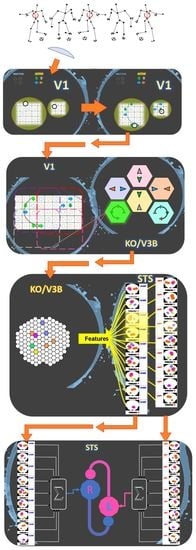
2. Model

2.1. Local Motion Energy Detectors
2.2. Opponent-Motion Detectors
2.3. Complex Global Optical-Flow Patterns
2.4. Complete Biological Motion Pattern Detectors (Motion Pattern Detectors)
2.5. Robust Mutual Inhibition Model
2.6. Modeling of the Internal Noise
3. Methods
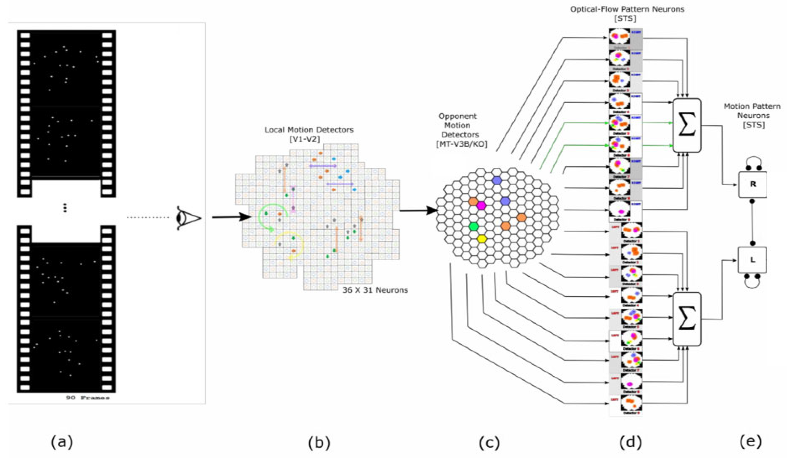
3.1. Stimuli and Data
3.2. Local Motion Energy and Opponent Motion Neurons
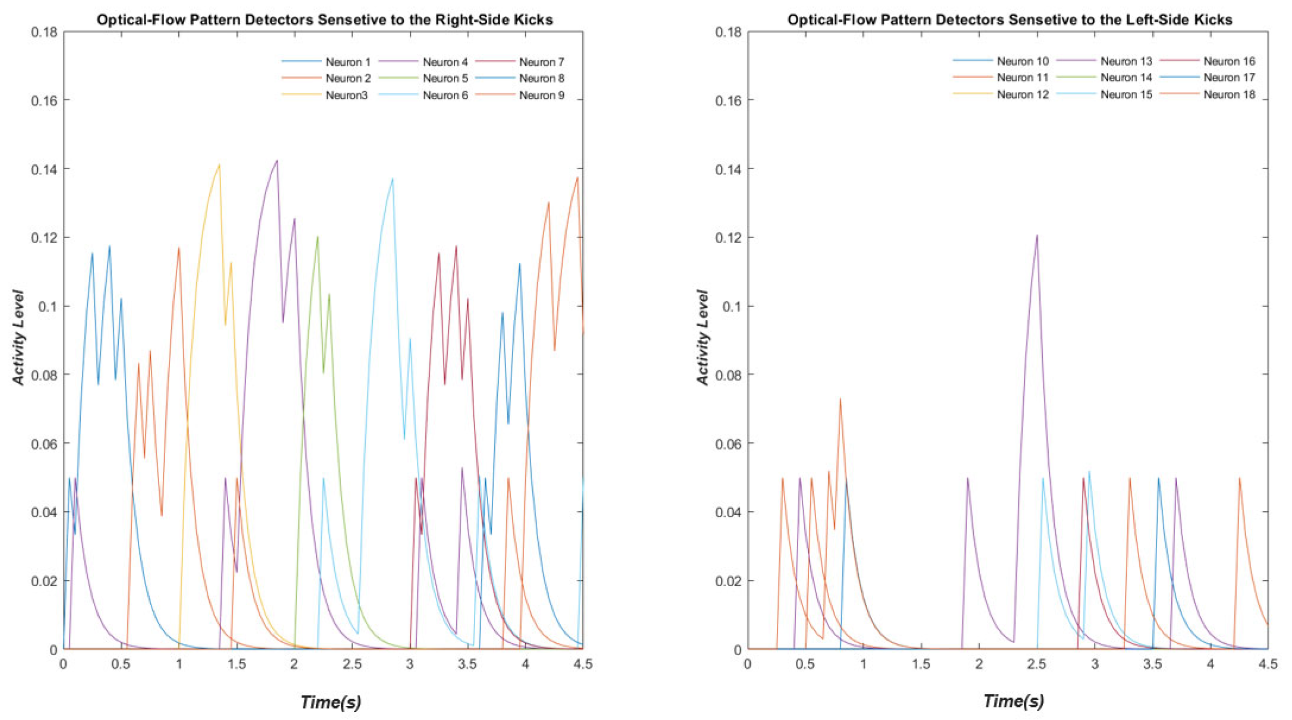
3.3. Optic Flow Pattern Neurons
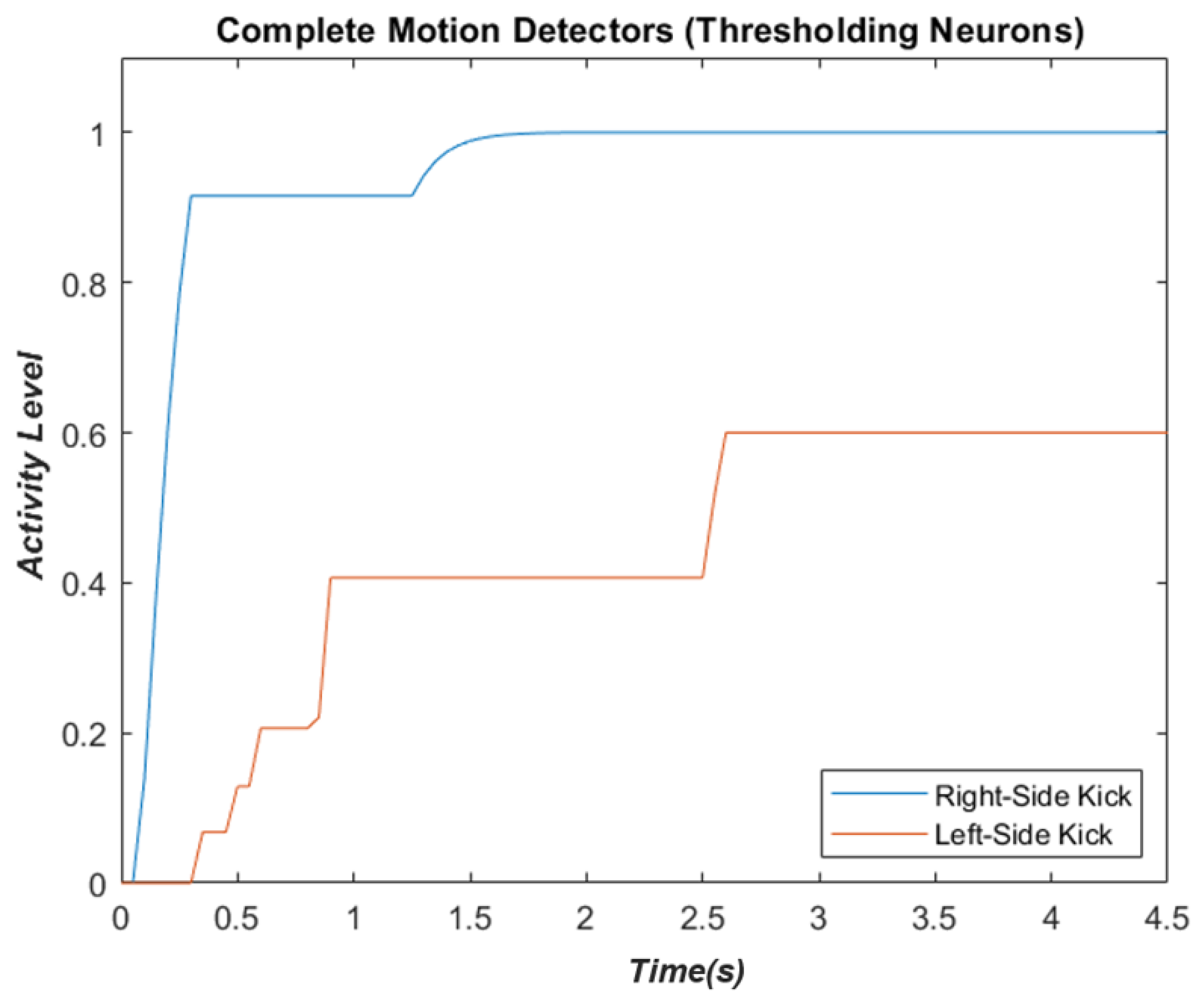
3.4. Motion-Pattern Neurons
3.5. Simulating Human Behavior
- 1.
- The standard deviation of the added internal noise, .
- 2.
- The time constant, .
- 3.
- The inhibitory feedback gain, .
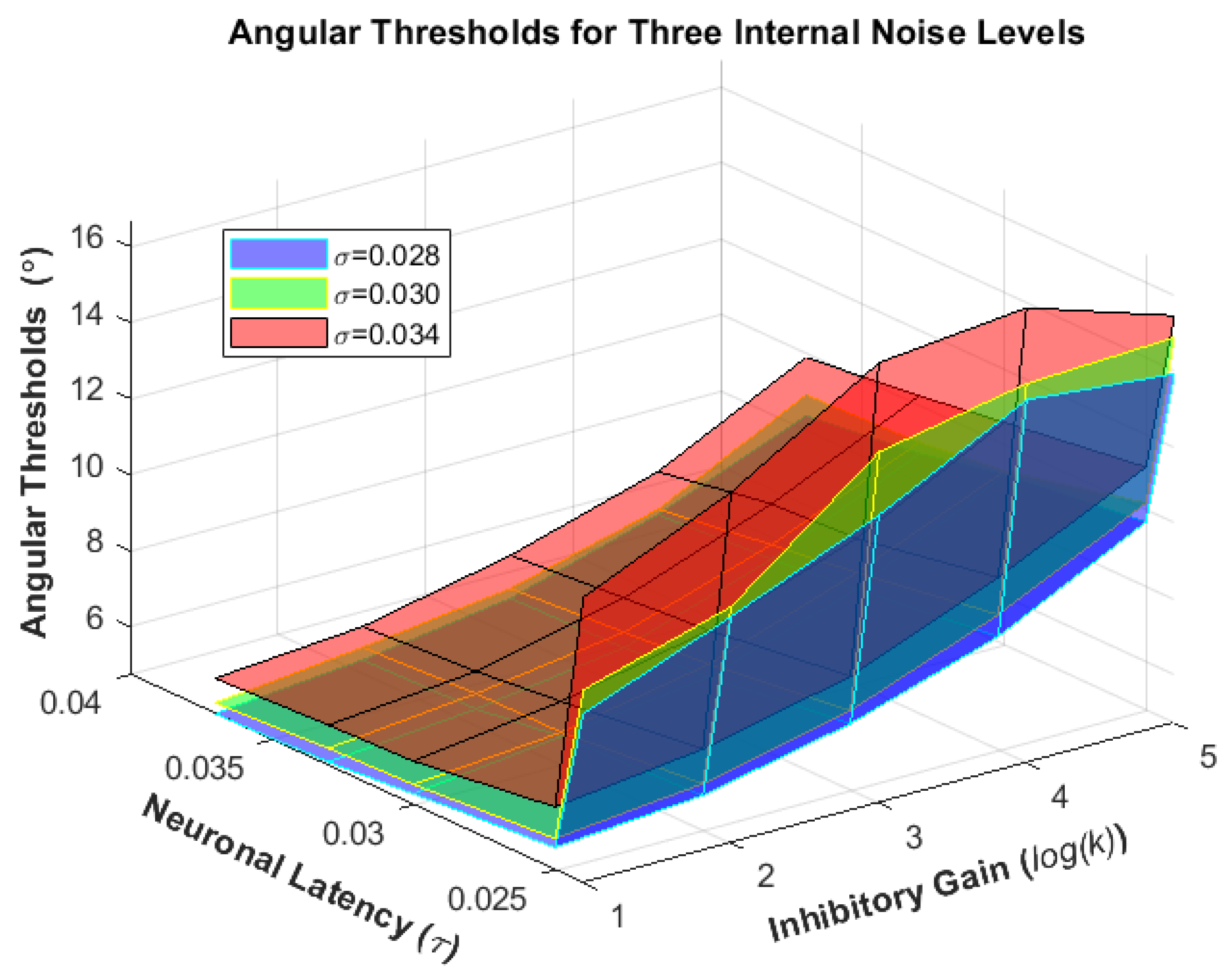
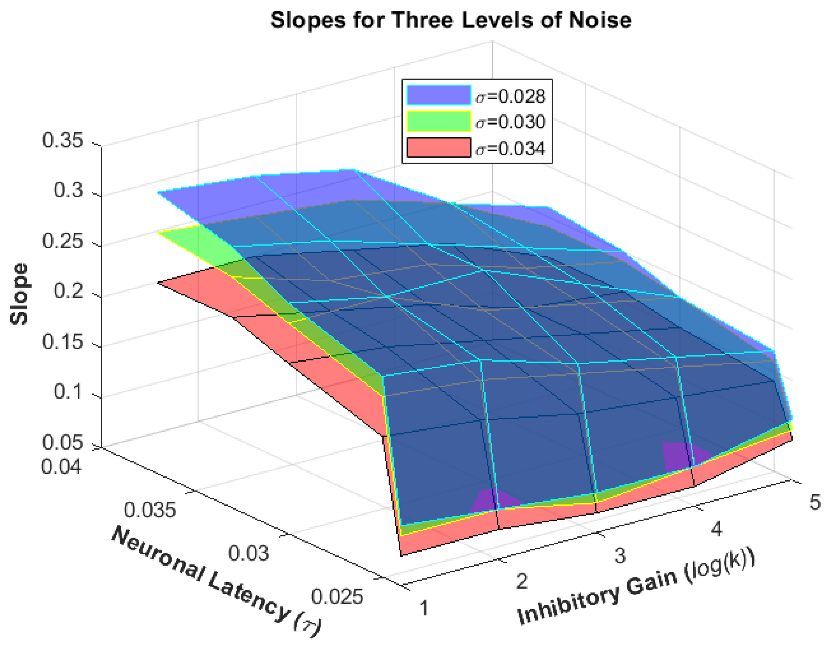
4. Results
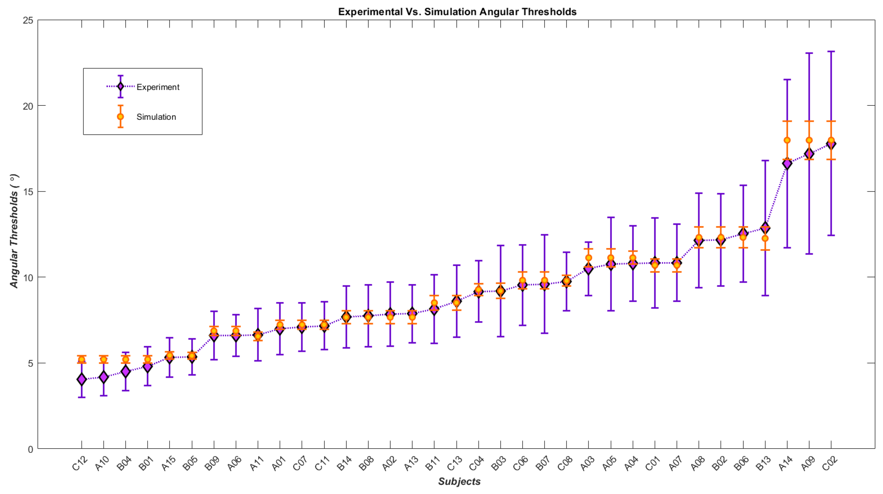
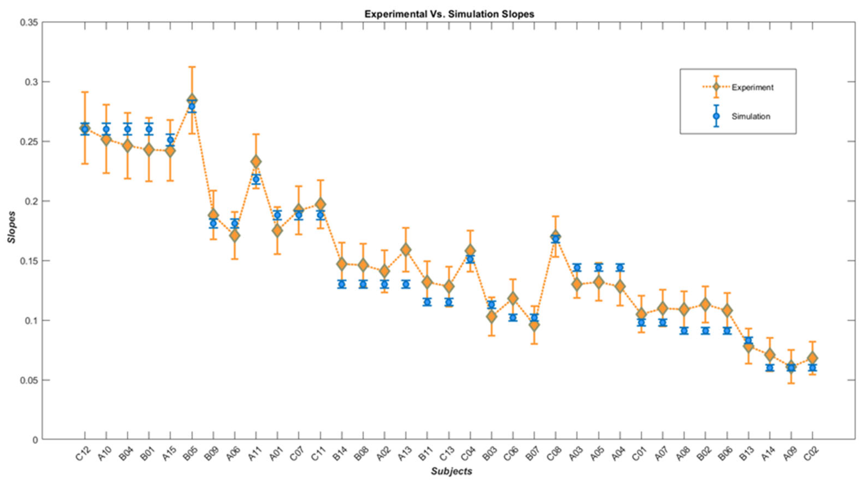
Human Results vs. Simulation Results
5. Discussion
Author Contributions
Funding
Institutional Review Board Statement
Informed Consent Statement
Data Availability Statement
Conflicts of Interest
References
- Blake, R.; Shiffrar, M. Perception of Human Motion. Annu. Rev. Psychol. 2007, 58, 47–73. [Google Scholar] [CrossRef] [PubMed]
- Giese, M.A.; Poggio, T. Neural mechanisms for the recognition of biological movements. Nat. Rev. Neurosci. 2003, 4, 179–192. [Google Scholar] [CrossRef] [PubMed]
- Beintema, J.A.; Lappe, M. Perception of biological motion without local image motion. Proc. Natl. Acad. Sci. USA 2002, 99, 5661–5663. [Google Scholar] [CrossRef] [PubMed]
- Mather, G.; Radford, K.; West, S. Low-level visual processing of biological motion. Proc. R. Soc. B Boil. Sci. 1992, 249, 149–155. [Google Scholar] [CrossRef]
- Casile, A.; Giese, M.A. Critical features for the recognition of biological motion. J. Vis. 2005, 5, 6–60. [Google Scholar] [CrossRef]
- Chang, D.H.F.; Troje, N. The local inversion effect in biological motion perception is acceleration-based. J. Vis. 2008, 8, 911. [Google Scholar] [CrossRef]
- Troje, N.F.; Westhoff, C. The inversion effect in biological motion perception: Evidence for a “life detector”? Curr. Biol. 2006, 16, 821–824. [Google Scholar] [CrossRef]
- Bardi, L.; Regolin, L.; Simion, F. Biological motion preference in humans at birth: Role of dynamic and configural properties. Dev. Sci. 2010, 14, 353–359. [Google Scholar] [CrossRef]
- Vallortigara, G.; Regolin, L.; Marconato, F. Visually Inexperienced Chicks Exhibit Spontaneous Preference for Biological Motion Patterns. PLoS Biol. 2005, 3, e208. [Google Scholar] [CrossRef]
- Thurman, S.; Lu, H. Bayesian integration of position and orientation cues in perception of biological and non-biological forms. Front. Hum. Neurosci. 2014, 8, 91. [Google Scholar] [CrossRef]
- Grosbras, M.-H.; Beaton, S.; Eickhoff, S.B. Brain regions involved in human movement perception: A quantitative voxel-based meta-analysis. Hum. Brain Mapp. 2012, 33, 431–454. [Google Scholar] [CrossRef]
- Kourtzi, Z.; Krekelberg, B.; van Wezel, R.J. Linking form and motion in the primate brain. Trends Cogn. Sci. 2008, 12, 230–236. [Google Scholar] [CrossRef]
- Gilaie-Dotan, S.; Saygin, A.P.; Lorenzi, L.J.; Rees, G.; Behrmann, M. Ventral aspect of the visual form pathway is not critical for the perception of biological motion. Proc. Natl. Acad. Sci. USA 2015, 112, E361–E370. [Google Scholar] [CrossRef]
- Bitzer, S.; Park, H.; Blankenburg, F.; Kiebel, S.J. Perceptual decision making: Drift-diffusion model is equivalent to a Bayesian model. Front. Hum. Neurosci. 2014, 8, 102. [Google Scholar] [CrossRef]
- Kahneman, D.; Tversky, A. Prospect theory: An analysis of decision under risk. In Handbook of the Fundamentals of Financial Decision Making: Part I; World Scientific: Singapore, 2013; pp. 99–127. [Google Scholar]
- Braun, D.A.; Nagengast, A.J.; Wolpert, D.M. Risk-Sensitivity in Sensorimotor Control. Front. Hum. Neurosci. 2011, 5, 1. [Google Scholar] [CrossRef]
- Dayan, P.; Niv, Y. Reinforcement learning: The Good, The Bad and The Ugly. Curr. Opin. Neurobiol. 2008, 18, 185–196. [Google Scholar] [CrossRef]
- Nagengast, A.J.; Braun, D.A.; Wolpert, D.M. Risk-Sensitive Optimal Feedback Control Accounts for Sensorimotor Behavior under Uncertainty. PLoS Comput. Biol. 2010, 6, e1000857. [Google Scholar] [CrossRef]
- Niv, Y.; Edlund, J.A.; Dayan, P.; O’Doherty, J.P. Neural Prediction Errors Reveal a Risk-Sensitive Reinforcement-Learning Process in the Human Brain. J. Neurosci. 2012, 32, 551–562. [Google Scholar] [CrossRef]
- Shen, Y.; Tobia, M.; Sommer, T.; Obermayer, K. Risk-Sensitive Reinforcement Learning. Neural Comput. 2014, 26, 1298–1328. [Google Scholar] [CrossRef]
- Lugo, J.E.; Mejia-Romero, S.; Doti, R.; Ray, K.; Kothari, S.L.; Withers, G.S.; Faubert, J. A simple dynamic model that accounts for regulation of neuronal polarity. J. Integr. Neurosci. 2018, 17, 323–330. [Google Scholar]
- Romeas, T.; Faubert, J. Soccer athletes are superior to non-athletes at perceiving soccer-specific and non-sport specific human biological motion. Front. Psychol. 2015, 6, 1343. [Google Scholar] [CrossRef] [PubMed]
- Smith, A.T.; Snowden, R.J. Visual Detection of Motion; Academic Press: New York, NY, USA, 1994. [Google Scholar]
- Allman, J.; Miezin, F.; McGuinness, E. Direction- and Velocity-Specific Responses from beyond the Classical Receptive Field in the Middle Temporal Visual Area (MT). Perception 1985, 14, 105–126. [Google Scholar] [CrossRef] [PubMed]
- Gawne, T.J.; Martin, J.M. Responses of Primate Visual Cortical Neurons to Stimuli Presented by Flash, Saccade, Blink, and External Darkening. J. Neurophysiol. 2002, 88, 2178–2186. [Google Scholar] [CrossRef]
- Lampl, I.; Ferster, D.; Poggio, T.; Riesenhuber, M. Intracellular Measurements of Spatial Integration and the MAX Operation in Complex Cells of the Cat Primary Visual Cortex. J. Neurophysiol. 2004, 92, 2704–2713. [Google Scholar] [CrossRef] [PubMed]
- Riesenhuber, M.; Poggio, T. Hierarchical models of object recognition in cortex. Nat. Neurosci. 1999, 2, 1019–1025. [Google Scholar] [CrossRef]
- Orban, G.A.; Dupont, P.; De Bruyn, B.; Vogels, R.; Vandenberghe, R.; Mortelmans, L. A motion area in human visual cortex. Proc. Natl. Acad. Sci. USA 1995, 92, 993–997. [Google Scholar] [CrossRef]
- Orban, G.A.; Lagae, L.; Verri, A.; Raiguel, S.; Xiao, D.; Maes, H.; Torre, V. First-order analysis of optical flow in monkey brain. Proc. Natl. Acad. Sci. USA 1992, 89, 2595–2599. [Google Scholar] [CrossRef]
- Mineiro, P.; Zipser, D. Analysis of Direction Selectivity Arising from Recurrent Cortical Interactions. Neural Comput. 1998, 10, 353–371. [Google Scholar] [CrossRef]
- Theodoridis, S. Introduction to Pattern Recognition: A MATLAB Approach; Academic Press: Amsterdam, The Netherlands, 2010. [Google Scholar]
- Decety, J.; Grèzes, J. Neural mechanisms subserving the perception of human actions. Trends Cogn. Sci. 1999, 3, 172–178. [Google Scholar] [CrossRef]
- Oram, M.W.; Perrett, D.I. Responses of Anterior Superior Temporal Polysensory (STPa) Neurons to “Biological Motion” Stimuli. J. Cogn. Neurosci. 1994, 6, 99–116. [Google Scholar] [CrossRef]
- Perrett, D.; Smith, P.; Mistlin, A.; Chitty, A.; Head, A.; Potter, D.; Broennimann, R.; Milner, A.; Jeeves, M. Visual analysis of body movements by neurones in the temporal cortex of the macaque monkey: A preliminary report. Behav. Brain Res. 1985, 16, 153–170. [Google Scholar] [CrossRef]
- Vaina, L.M.; Solomon, J.; Chowdhury, S.; Sinha, P.; Belliveau, J.W. Functional neuroanatomy of biological motion perception in humans. Proc. Natl. Acad. Sci. USA 2001, 98, 11656–11661. [Google Scholar] [CrossRef]
- Grossman, E.; Donnelly, M.; Price, R.; Pickens, D.; Morgan, V.; Neighbor, G.; Blake, R. Brain Areas Involved in Perception of Biological Motion. J. Cogn. Neurosci. 2000, 12, 711–720. [Google Scholar] [CrossRef]
- Wilson, H.R. Spikes, Decisions, and Actions: The Dynamical Foundations of Neurosciences; Oxford University Press: Oxford, UK, 1999. [Google Scholar]
- Jung, Y.; Hu, J. AK-fold averaging cross-validation procedure. J. Nonparametric Stat. 2015, 27, 167–179. [Google Scholar] [CrossRef]
- Hill, E.L. Executive dysfunction in autism. Trends Cogn. Sci. 2004, 8, 26–32. [Google Scholar] [CrossRef]
- Hosenbocus, S.; Chahal, R. A review of executive function deficits and pharmacological management in children and adolescents. J. Can. Acad. Child Adolesc. Psychiatry 2012, 21, 223. [Google Scholar]
- Rubenstein, J.L.R.; Merzenich, M.M. Model of autism: Increased ratio of excitation/inhibition in key neural systems. Genes Brain Behav. 2003, 2, 255–267. [Google Scholar] [CrossRef]


| Subjects | Angular Thresholds from Experiment | Angular Thresholds from Simulation | Slopes from Experiment | Slopes from Simulation | Inhibitory Gain | Time Constant | Noise |
|---|---|---|---|---|---|---|---|
| C12 | 4.041 ± 1.05 | 5.209 ± 0.200 | 0.261 ± 0.03 | 0.260 ± 0.0048 | 4 | 0.0245 | 0.022 |
| A10 | 4.176 ± 1.08 | ˶ | 0.252 ± 0.028 | ˶ | ˶ | ˶ | ˶ |
| B04 | 4.506 ± 1.1 | ˶ | 0.246 ± 0.027 | ˶ | ˶ | ˶ | ˶ |
| B01 | 4.805 ± 1.12 | ˶ | 0.243 ± 0.026 | ˶ | ˶ | ˶ | ˶ |
| A15 | 5.321 ± 1.14 | 5.448 ± 0.205 | 0.242 ± 0.025 | 0.251 ± 0.0047 | 2 | 0.033 | 0.032 |
| B05 | 5.361 ± 1.04 | 5.425 ± 0.193 | 0.284 ± 0.028 | 0.279 ± 0.005 | 4 | 0.037 | 0.03 |
| B09 | 6.602 ± 1.41 | 6.871 ± 0.268 | 0.188 ± 0.02 | 0.181 ± 0.0036 | 4 | 0.025 | 0.034 |
| A11 | 6.637 ± 1.52 | ˶ | 0.171 ± 0.019 | ˶ | ˶ | ˶ | ˶ |
| A06 | 6.609 ± 1.21 | 6.556 ± 0.232 | 0.233 ± 0.022 | 0.218 ± 0.004 | 8 | 0.033 | 0.032 |
| A01 | 7.000 ± 1.51 | 7.228 ± 0.263 | 0.175 ± 0.019 | 0.188 ± 0.0036 | 8 | 0.03 | 0.034 |
| C07 | 7.097 ± 1.42 | ˶ | 0.192 ± 0.02 | ˶ | ˶ | ˶ | ˶ |
| C11 | 7.165 ± 1.39 | ˶ | 0.197 ± 0.02 | ˶ | ˶ | ˶ | ˶ |
| B14 | 7.692 ± 1.79 | 7.664 ± 0.363 | 0.147 ± 0.017 | 0.130 ± 0.0031 | 1 | 0.024 | 0.026 |
| B08 | 7.753 ± 1.8 | ˶ | 0.146 ± 0.017 | ˶ | ˶ | ˶ | ˶ |
| A02 | 7.837 ± 1.86 | ˶ | 0.141 ± 0.017 | ˶ | ˶ | ˶ | ˶ |
| A13 | 7.873 ± 1.69 | ˶ | 0.159 ± 0.018 | ˶ | ˶ | ˶ | ˶ |
| B11 | 8.132 ± 2 | 8.509 ± 0.421 | 0.132 ± 0.017 | 0.115 ± 0.003 | 1 | 0.024 | 0.028 |
| C13 | 8.594 ± 2.08 | ˶ | 0.128 ± 0.016 | ˶ | ˶ | ˶ | ˶ |
| C04 | 9.173 ± 1.77 | 9.275 ± 0.337 | 0.158 ± 0.017 | 0.151 ± 0.003 | 16 | 0.025 | 0.034 |
| B03 | 9.191 ± 2.64 | 9.198 ± 0.438 | 0.103 ± 0.016 | 0.113 ± 0.0029 | 2 | 0.024 | 0.028 |
| C06 | 9.543 ± 2.34 | 9.818 ± 0.496 | 0.118 ± 0.016 | 0.102 ± 0.0028 | 2 | 0.024 | 0.03 |
| B07 | 9.589 ± 2.86 | ˶ | 0.096 ± 0.015 | ˶ | ˶ | ˶ | ˶ |
| C08 | 9.747 ± 1.69 | 9.791 ± 0.313 | 0.170 ± 0.017 | 0.168 ± 0.0031 | 32 | 0.033 | 0.032 |
| A03 | 10.49 ± 1.56 | 11.131 ± 0.376 | 0.130 ± 0.011 | 0.144 ± 0.0028 | 32 | 0.025 | 0.34 |
| A04 | 10.801 ± 2.2 | ˶ | 0.132 ± 0.015 | ˶ | ˶ | ˶ | ˶ |
| A07 | 10.843 ± 2.25 | ˶ | 0.128 ± 0.015 | ˶ | ˶ | ˶ | ˶ |
| A05 | 10.77 ± 2.71 | 10.696 ± 0.529 | 0.105 ± 0.015 | 0.098 ± 0.0028 | 4 | 0.024 | 0.028 |
| C01 | 10.83 ± 2.6 | ˶ | 0.110 ± 0.015 | ˶ | ˶ | ˶ | ˶ |
| A08 | 12.132 ± 2.75 | 12.315 ± 0.606 | 0.109 ± 0.015 | 0.091 ± 0.0027 | 8 | 0.024 | 0.028 |
| B02 | 12.173 ± 2.67 | ˶ | 0.113 ± 0.015 | ˶ | ˶ | ˶ | ˶ |
| B06 | 12.525 ± 2.81 | ˶ | 0.108 ± 0.014 | ˶ | ˶ | ˶ | ˶ |
| B13 | 12.86 ± 3.93 | 12.258 ± 0.664 | 0.078 ± 0.014 | 0.083 ± 0.0027 | 2 | 0.024 | 0.034 |
| A14 | 16.617 ± 4.88 | 17.978 ± 1.105 | 0.071 ± 0.013 | 0.06 ± 0.0025 | 8 | 0.024 | 0.036 |
| A09 | 17.194 ± 5.84 | ˶ | 0.061 ± 0.013 | ˶ | ˶ | ˶ | ˶ |
| C02 | 17.787 ± 5.35 | ˶ | 0.068 ± 0.013 | ˶ | ˶ | ˶ | ˶ |
Publisher’s Note: MDPI stays neutral with regard to jurisdictional claims in published maps and institutional affiliations. |
© 2022 by the authors. Licensee MDPI, Basel, Switzerland. This article is an open access article distributed under the terms and conditions of the Creative Commons Attribution (CC BY) license (https://creativecommons.org/licenses/by/4.0/).
Share and Cite
Misaghian, K.; Lugo, J.E.; Faubert, J. “Descriptive Risk-Averse Bayesian Decision-Making,” a Model for Complex Biological Motion Perception in the Human Dorsal Pathway. Biomimetics 2022, 7, 193. https://doi.org/10.3390/biomimetics7040193
Misaghian K, Lugo JE, Faubert J. “Descriptive Risk-Averse Bayesian Decision-Making,” a Model for Complex Biological Motion Perception in the Human Dorsal Pathway. Biomimetics. 2022; 7(4):193. https://doi.org/10.3390/biomimetics7040193
Chicago/Turabian StyleMisaghian, Khashayar, Jesus Eduardo Lugo, and Jocelyn Faubert. 2022. "“Descriptive Risk-Averse Bayesian Decision-Making,” a Model for Complex Biological Motion Perception in the Human Dorsal Pathway" Biomimetics 7, no. 4: 193. https://doi.org/10.3390/biomimetics7040193
APA StyleMisaghian, K., Lugo, J. E., & Faubert, J. (2022). “Descriptive Risk-Averse Bayesian Decision-Making,” a Model for Complex Biological Motion Perception in the Human Dorsal Pathway. Biomimetics, 7(4), 193. https://doi.org/10.3390/biomimetics7040193