Figure 1.
A diagram of the electrical measurement tool for recording extracellular potentials from proteinoid assemblies. The setup has a glass vial with rehydrated proteinoid samples. These samples can be microspheres, fibers, or a 50:50 v/v mixture. There are eight pairs of Pt/Ir electrodes placed 10 mm apart. Electrodes are connected to an ADC-24 PicoLog data logger operating in differential mode with a sampling rate of 1 sample per second. The central ground electrode provides a common reference point for all measurements. This setup allows for 50 to 100 h of recording at a stable temperature of 25 ± 1 °C. It captures quick electrical events and shows long-term patterns.
Figure 2.
Changes in electrical potentials of Glu-Phe-Asp (GFD) proteinoid microspheres in starch medium observed over about 48 h (175,000 s). The starch medium changes the electrical response seen in pure GFD microsphere preparations. Instead of sharp spikes, it causes gradual drift patterns across several recording channels. Channel 4 (gray) shows a pronounced decline from +75 mV to +20 mV, while Channel 7 (pink) maintains a strong negative potential around −100 mV throughout the recording. The lack of action potential spikes and burst patterns in this control experiment shows that the electrical behaviors in pure GFD systems are true traits of the proteinoid structures. They are not just measurement errors. This control shows how the surrounding medium can change the electrochemical gradients created by GFD assemblies.
Figure 3.
Raman spectra display intensity as a function of wavenumber (cm−1) for the (a) microspheres, (b) fibers, and (c) the fibers and microspheres composite. The spectral range spans from 100 to 1999 cm−1. Key vibrational modes are observed at 1250 cm−1 (amide III) and 1650 cm−1 (amide I), corresponding to characteristic features of the proteinoid backbone structure. Microspheres exhibit broader and more intense peaks, indicating a higher degree of molecular disorder. In contrast, fibers show sharper peaks, reflecting a more ordered molecular arrangement. The composite spectrum presents a combination of both morphologies, suggesting that this structural blend may enhance the material’s applicability in biomaterials where a balance of order and flexibility is beneficial.
Figure 4.
Temporal changes in extracellular potentials recorded from a mixture of Glu-Phe-Asp (GFD) microspheres and fibers in a 50:50 v/v ratio. Multiple recording channels (ChA–ChI) reveal distinct electrophysiological profiles across the sample. The system shows initial changes from 0 to 10,000 s. It stabilizes over time. The steady-state potentials range from −40 mV to +45 mV. Channel E (purple) has a steady positive potential of about +45 mV. In contrast, Channel H (light blue) stabilizes at around −25 mV. Intermediate channels show different equilibration patterns. Some channels, like ChI (brown), have metastable plateaus around +15 mV. This varied electrical behaviour hints at different functional areas in the microsphere–fiber network. These areas may link to the shapes of the fibrillar and spherical structures. The long-term stability observed (over 60,000 s) shows that strong electrochemical gradients form in the mixed GFD assembly. This is typical of the extracellular field potentials created by self-assembling peptide structures.
![Biomimetics 10 00360 g004]()
Figure 5.
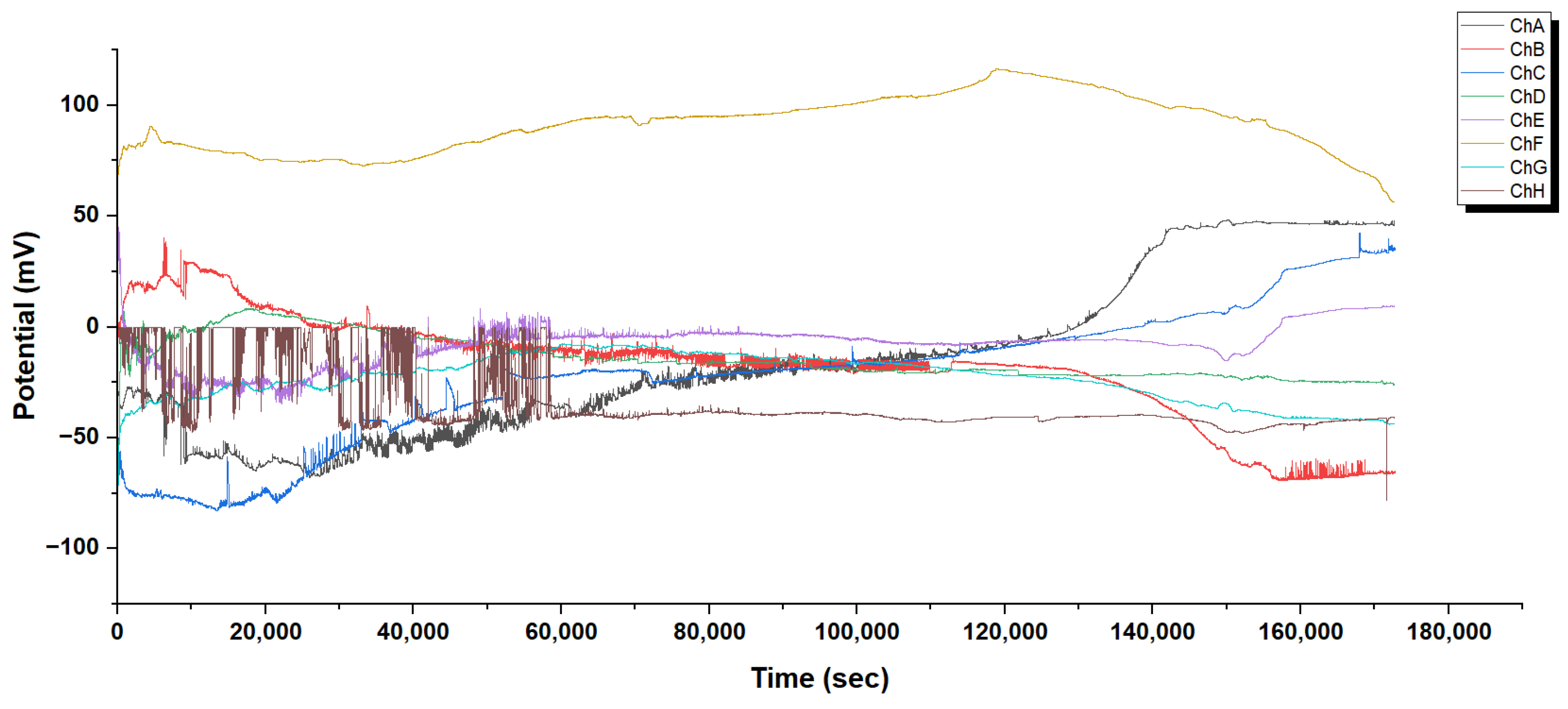
Long-term recordings show electrical activity from pure Glu-Phe-Asp (GFD) microspheres. They display complex spiking dynamics over about 50 h, or 180,000 s. The recording shows three clear phases of electrophysiological behaviour. In the initial phase (0–40,000 s), high-frequency spiking occurs, especially in channels B, E, and G. Spike amplitudes range from 5–15 mV, and bursts have distinct patterns. In the transitional phase, (40,000–120,000 s), there is a gradual change in potential trajectories. Spiking frequency decreases during this time. In the late phase (120,000–180,000 s), channels spread across a wide potential range of −70 to +110 mV. Channel-specific spiking patterns, especially in channel B at −70 mV, become noticeable. Channel F (yellow) stays at high potentials during the recording, peaking at +110 mV. Other channels, however, show shifts between positive and negative values. This spontaneous spiking behaviour shows a key difference from GFD fiber structures. GFD fibers have smooth, steady potential changes and do not show action potential-like events. Spikes appear only in microsphere preparations. Their round shape helps create the electrochemical compartments. This shape allows for quick ionic flows across their surfaces. In contrast, fibers have a long, non-compartmentalized structure. This shape prevents the fast potential changes that spikes need to form.
Figure 5.
Long-term recordings show electrical activity from pure Glu-Phe-Asp (GFD) microspheres. They display complex spiking dynamics over about 50 h, or 180,000 s. The recording shows three clear phases of electrophysiological behaviour. In the initial phase (0–40,000 s), high-frequency spiking occurs, especially in channels B, E, and G. Spike amplitudes range from 5–15 mV, and bursts have distinct patterns. In the transitional phase, (40,000–120,000 s), there is a gradual change in potential trajectories. Spiking frequency decreases during this time. In the late phase (120,000–180,000 s), channels spread across a wide potential range of −70 to +110 mV. Channel-specific spiking patterns, especially in channel B at −70 mV, become noticeable. Channel F (yellow) stays at high potentials during the recording, peaking at +110 mV. Other channels, however, show shifts between positive and negative values. This spontaneous spiking behaviour shows a key difference from GFD fiber structures. GFD fibers have smooth, steady potential changes and do not show action potential-like events. Spikes appear only in microsphere preparations. Their round shape helps create the electrochemical compartments. This shape allows for quick ionic flows across their surfaces. In contrast, fibers have a long, non-compartmentalized structure. This shape prevents the fast potential changes that spikes need to form.
![Biomimetics 10 00360 g005]()
Figure 6.
We conduct a high-resolution analysis of spike waveforms in Glu-Phe-Asp microsphere networks. This analysis spans multiple recording channels. (a) Channel A shows quick upward spikes of 2–4 mV on a slowly rising baseline of −29 to −24 mV. The spikes become more common and larger as the recording continues. (b) Channel B shows clear, downward spikes with an amplitude of 2–3 mV. After 170,000 s, it shifts to a steadier baseline with fewer spikes. (c) Channel C displays clear, large spikes (3–5 mV) that stand out from a slowly rising baseline (−25 to −19 mV). The waveforms have a quick rise and a gradual decay. (d) Channel D shows step-like changes between stable potential states (−13 to −17 mV). There are sudden shifts, followed by flat periods, which indicate clear state transitions. (e) Channel E shows complex two-way spiking. It has large swings, reaching 8–10 mV. It also features long plateaus at various potential levels. This behaviour indicates bistable switching. (f) Channel H displays high-frequency spikes with small amplitudes (1–2 mV). These spikes sit on a fluctuating baseline that ranges from −42 to −36 mV. Additionally, there are periodic bursts. These different spiking patterns are very unlike the steady potential changes in fibrillar structures. This shows how the shape of microspheres creates separate areas that can quickly move ions across boundaries. This movement leads to action potential-like events, featuring distinct depolarization and repolarization phases. The differences in spike shape across channels show that there are local variations in electrochemical properties in the microsphere network. This might allow for complex information processing through the integration of signals over space and time.
![Biomimetics 10 00360 g006]()
Figure 7.
We recorded extracellular potentials from pure Glu-Phe-Asp (GFD) fiber networks for about 100 h, or 360,000 s. These long-term recordings showed unique electrophysiological dynamics without classical spiking activity. The temporal evolution shows three main phases. In the initial high-amplitude transient phase (0–50,000 s), there are large potential changes. Channels D and F reach peaks of +200 mV and +100 mV. In the transition phase (50,000–150,000 s), channels start to align their potential positions. In the extended equilibrium phase (150,000–360,000 s), stability is key, with very few fluctuations. GFD fibers do not show rapid spike events like microsphere preparations do. Instead, they have smooth, gradual potential changes. This matches the distributed ionic gradients found in their long fiber structures. The recordings show clear polarization bands. Channels split into three groups, as follows. Positive: Channels C, E, F (+40 to +65 mV). Neutral: Channels A, B, H (−10 to +30 mV). Negative: Channel G (−60 to −90 mV) This separation of potentials shows that the fiber network has different functions, even though it looks the same. The stability of these distributions lasts over 200,000 s. This shows that strong electrochemical gradients form and persist. This is due to the fibrillar structure. These gradients can store information long-term. This is different from the dynamic signals in microsphere systems.
![Biomimetics 10 00360 g007]()
Figure 8.
High-resolution temporal analysis of Glu-Phe-Asp fiber network activity from Channel F recordings at different time points. (a) Early recording (54,000–74,000 s) shows a gradual rise in potential. It rises from about 41 mV to 47 mV. You can see micro-oscillations with amplitudes of 0.5–1.0 mV. There are no clear spiking events. The steady rise ( mV over 20,000 s) shows a gradual buildup of charge in the fiber structure. The small-amplitude fluctuations reflect ionic movements spread out across the area, not isolated discharge events. (b) Middle-phase recording (180,000–225,000 s) shows new quasi-periodic oscillations. These oscillations have peak-to-peak amplitudes of 3–5 mV. The periodicity varies, with major troughs occurring about every 5000–10,000 s. Slow-wave oscillations keep baseline potentials between 46 and 53 mV. They have uneven waveforms. The phases descend at a gradual pace and then rise rapidly. These fiber-specific oscillations occur over longer times than the quick spikes seen in microsphere preparations. This points to different mechanisms that control changes in fibrillar and spherical shapes. The long-lasting features of these oscillations suggest that ions move in large groups. This happens across the fiber network, not in small, quick bursts like in compartmentalized structures.
![Biomimetics 10 00360 g008]()
Figure 10.
SEM characterization of heterogeneous Glu-Phe-Asp (GFD) assemblies revealing microsphere–fiber interactions and morphological diversity. (a) Perforated microsphere (m) with central aperture (m) in direct contact with elongated fibrillar structure (length = m). Structural integration at the microsphere–fiber interface suggests possible electrochemical coupling between various domains. This was observed using an ETD detector with HV set to kV, magnification at 35,125×, HFW of m, and pressure at Torr. (b) High-resolution images show a microsphere with an uneven edge near fibrillar elements. This setup highlights the localized surface interactions at the shape’s boundary. The clear differences in electron density show varied compositional organization. This was observed using an ETD detector at HV = kV, with a magnification of 63,039×, an HFW of m, and a pressure of Torr. (c) The multi-generational microsphere assembly shows a size range with different sizes: m, m, m, and m. It also shows signs of budding-like growth. The spatial arrangement shows how the microsphere population develops. This was observed using an ETD detector at HV = kV, with magnification and an HFW of m. (d) The advanced-stage hollow microsphere structure (33.152 m) has smaller microspheres inside (1.5 m, 4.5 m). This shows a rare encapsulation phenomenon in synthetic self-assembling systems. The hierarchical setup has nested substructures. This design allows for compartmentalization of electrochemical processes. For example, consider the ETD detector. It operates at HV = kV with a magnification of . The HFW is m, and the pressure is Torr.
![Biomimetics 10 00360 g010]()
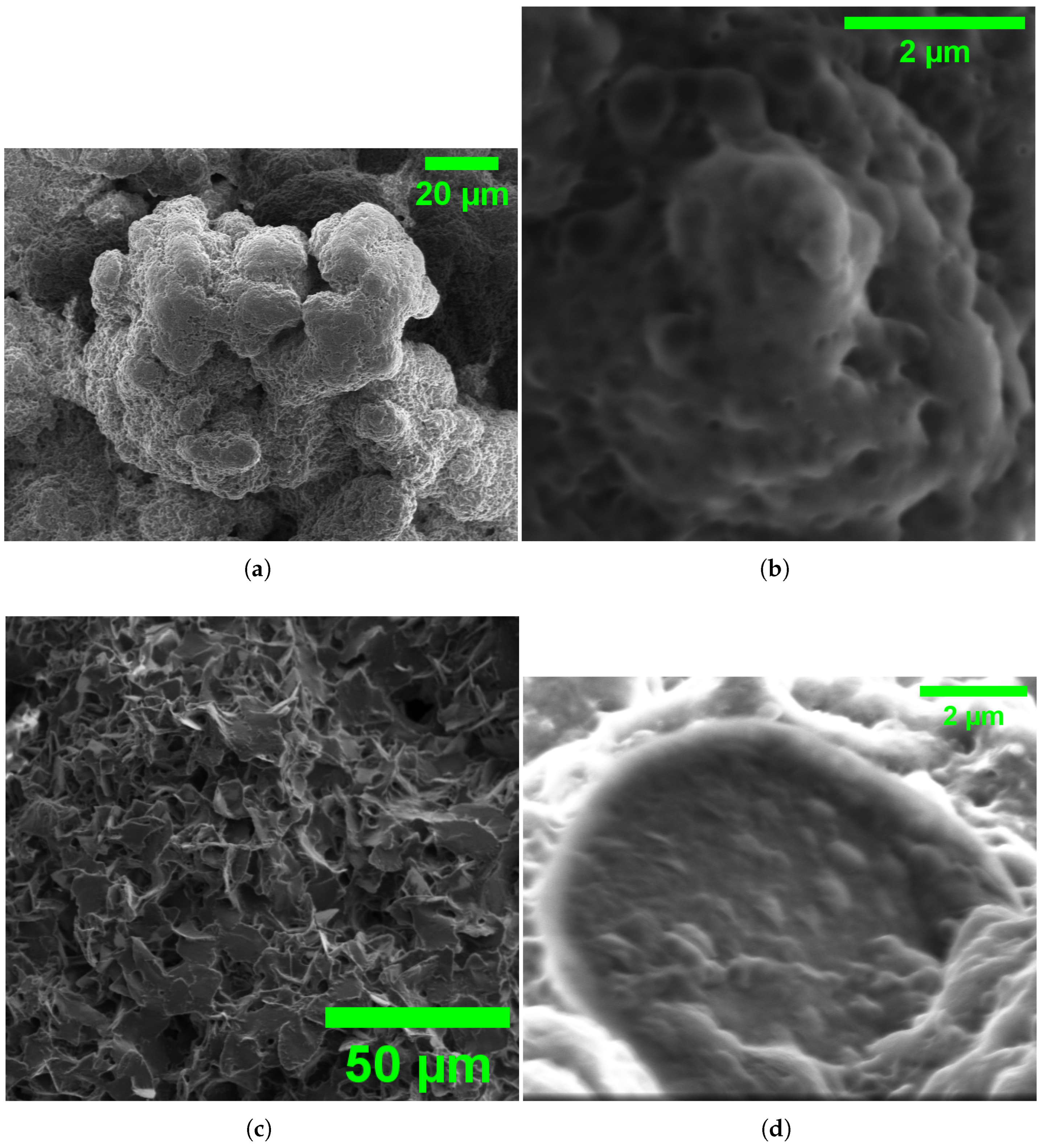
Figure 11.
Scanning electron microscopy (SEM) images of L-ASP morphology in water: (a) overview of aggregated L-ASP structures at 20 m scale, displaying a rough, clustered surface texture; (b) close-up view at 20 m scale, revealing complex surface details and porous features; (c) larger-scale view at 50 m, showing the distribution and uniformity of L-ASP particles; and (d) high-magnification image at 2 m, highlighting the fine nanoscale surface morphology and structural details of individual L-ASP particles.
Figure 12.
Changes in electrical properties of different GFD proteinoid structures over 1000 s. Capacitance (Cs/F) measurements show that fibrillar structures have much higher baseline values. The values are F for fibrillar (blue), F for microspheres (orange), and F for mixed morphologies (green). Microspheres show distinct transient capacitance spikes, reaching up to 162.514 F. This indicates quick charge buildup events. (b) Impedance (Z/Ohm) profiles show clear differences between morphologies. Microspheres have much higher impedance at Ohm. In contrast, fibers measure Ohm, while mixed systems are at Ohm. (c) Resistance (Idc/m) measurements show an inverse relationship with capacitance. Fibers have the highest resistance at 163,067.613 ± 9253.064 m. Next are mixed structures at 60,424.487 ± 1293.986 m. Finally, microspheres measure 15,830.739 ± 652.514 m. These unique electrical signatures relate to structure. Fibrillar shapes help spread charge but limit current flow. Microspheres allow ionic transport and keep high impedance. Mixed systems show traits in between, hinting at functional synergy among different structures.
![Biomimetics 10 00360 g012]()
Figure 13.
Bode plot of Glu-Phe-Asp proteinoids showing impedance magnitude (left axis, log scale) and phase (right axis) against frequency (log scale). This data is for fibers, microspheres, and the fibers and microspheres composite. Fibers show the lowest impedance, reaching as low as at high frequencies. This suggests they mainly behave resistively. This effect likely comes from better charge transport along their fibrous structures. Microspheres have the highest impedance, reaching values up to . They also show a phase shift near at Hz. This indicates a strong capacitive effect, likely from ionic interactions on their surface. The fibers and microspheres composite displays intermediate values, reflecting a balanced resistive–capacitive response. These trends show that fibers might work like a simple resistor. In contrast, microspheres probably fit a parallel RC circuit. This highlights their potential for custom uses in bioelectronics.
![Biomimetics 10 00360 g013]()
Figure 14.
Nyquist plots showing Glu-Phe-Asp proteinoids. They compare real impedance with negative imaginary impedance . The plots include (a) fibers and microspheres, (b) fibers, and (c) microspheres. Fibers show a compressed semicircle. The real part, , ranges from 0.180 to 0.181 k. The imaginary part, , goes from −0.015 to −0.008 k. This suggests a mainly resistive response. The charge transfer resistance is low, likely due to good ionic conduction along the fibers. Microspheres show a larger semicircle with ranging from 3.162 to 5.024 k. The values go from −4.492 to −4.064 k. This indicates strong capacitive impedance, like a parallel RC circuit. It could be caused by ionic interactions on the surface. The fibers + microspheres composite has a mid-range response. Its varies from 0.418 to 0.455 k, while ranges from −0.071 to −0.061 k. This indicates balanced resistive–capacitive behavior. One can zoom into specific regions of interest, such as fibers and microspheres (: 0.400 to 0.450 k, : −0.080 to −0.040 k), fibers (: 0.180 to 0.182 k, : −0.015 to −0.005 k), and microspheres (: 3.0 to 3.5 k, : −4.5 to −3.5 k), to explore detailed electrochemical dynamics for potential bioelectronic applications.
![Biomimetics 10 00360 g014]()
Figure 15.
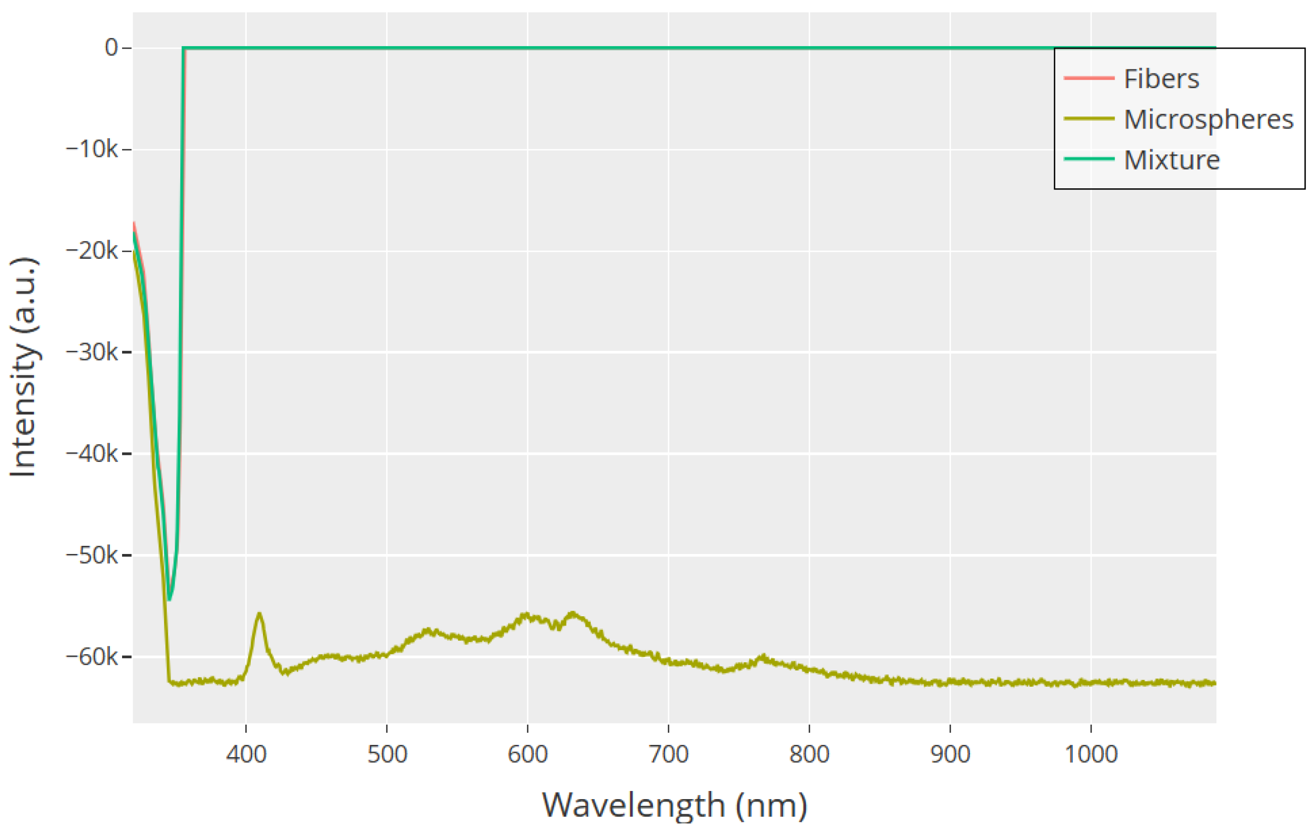
UV–Visible absorption spectra from 350 to 1050 nm show unique optical behaviors in GFD proteinoid morphologies. Microspheres (olive) keep their absorption profile, showing peaks at 410 nm and broad features from 500 to 650 nm. In contrast, fibers (red) and their mix with microspheres (teal) show surprising optical changes. The initial steep absorption edge at 350–375 nm represents – transitions in aromatic phenylalanine residues. The mixture makes a big change around 375 nm. It shifts from high absorption to complete transparency in the visible and near-infrared range. This strange optical behavior hints at complex interactions between light and matter in the mixed assembly. It may be linked to constructive and destructive interference at the interfaces of the microspheres and fibers. The sharp change also backs our idea. It shows that mixed shapes lead to unique electrical behaviors. This happens through cooperation among structural elements.
Figure 15.
UV–Visible absorption spectra from 350 to 1050 nm show unique optical behaviors in GFD proteinoid morphologies. Microspheres (olive) keep their absorption profile, showing peaks at 410 nm and broad features from 500 to 650 nm. In contrast, fibers (red) and their mix with microspheres (teal) show surprising optical changes. The initial steep absorption edge at 350–375 nm represents – transitions in aromatic phenylalanine residues. The mixture makes a big change around 375 nm. It shifts from high absorption to complete transparency in the visible and near-infrared range. This strange optical behavior hints at complex interactions between light and matter in the mixed assembly. It may be linked to constructive and destructive interference at the interfaces of the microspheres and fibers. The sharp change also backs our idea. It shows that mixed shapes lead to unique electrical behaviors. This happens through cooperation among structural elements.
Figure 16.
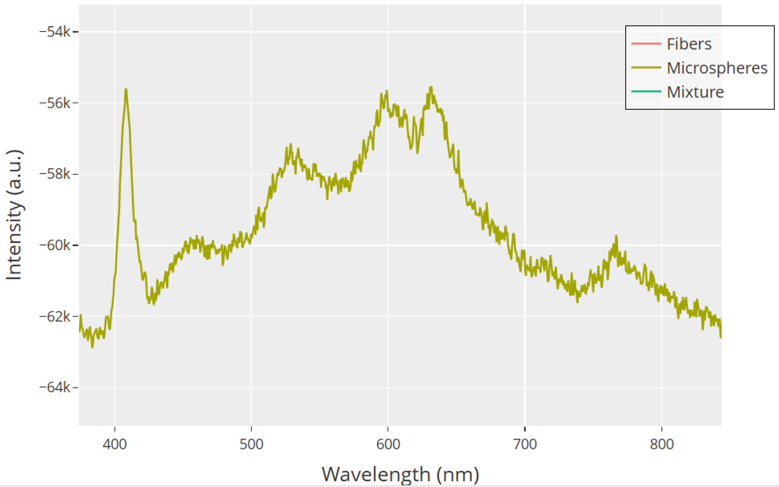
UV–Visible absorption spectra of Glu-Phe-Asp (GFD) proteinoid assemblies show clear spectroscopic signatures. These signatures vary across different morphologies in the 380–850 nm range. Microspheres (olive) show a complex spectrum with several absorption bands. There is a sharp peak at 410 nm. This peak likely comes from n– transitions of carbonyl groups. Broad absorption occurs between 570–630 nm, linked to electronic transitions in the peptide backbone. Additionally, a smaller feature at 750 nm may relate to extended conjugation networks. Fibers (red) and the 50:50 mixture (teal) have very different profiles. They overlap at lower wavelengths but diverge a lot past 400 nm. The mixture shows a flat response, which suggests aggregation-induced spectral damping. These unique spectral signatures match the various molecular patterns seen in SEM analysis. They also back up the structure-dependent electrical behaviors noted in our recordings.
Figure 16.
UV–Visible absorption spectra of Glu-Phe-Asp (GFD) proteinoid assemblies show clear spectroscopic signatures. These signatures vary across different morphologies in the 380–850 nm range. Microspheres (olive) show a complex spectrum with several absorption bands. There is a sharp peak at 410 nm. This peak likely comes from n– transitions of carbonyl groups. Broad absorption occurs between 570–630 nm, linked to electronic transitions in the peptide backbone. Additionally, a smaller feature at 750 nm may relate to extended conjugation networks. Fibers (red) and the 50:50 mixture (teal) have very different profiles. They overlap at lower wavelengths but diverge a lot past 400 nm. The mixture shows a flat response, which suggests aggregation-induced spectral damping. These unique spectral signatures match the various molecular patterns seen in SEM analysis. They also back up the structure-dependent electrical behaviors noted in our recordings.
Figure 17.
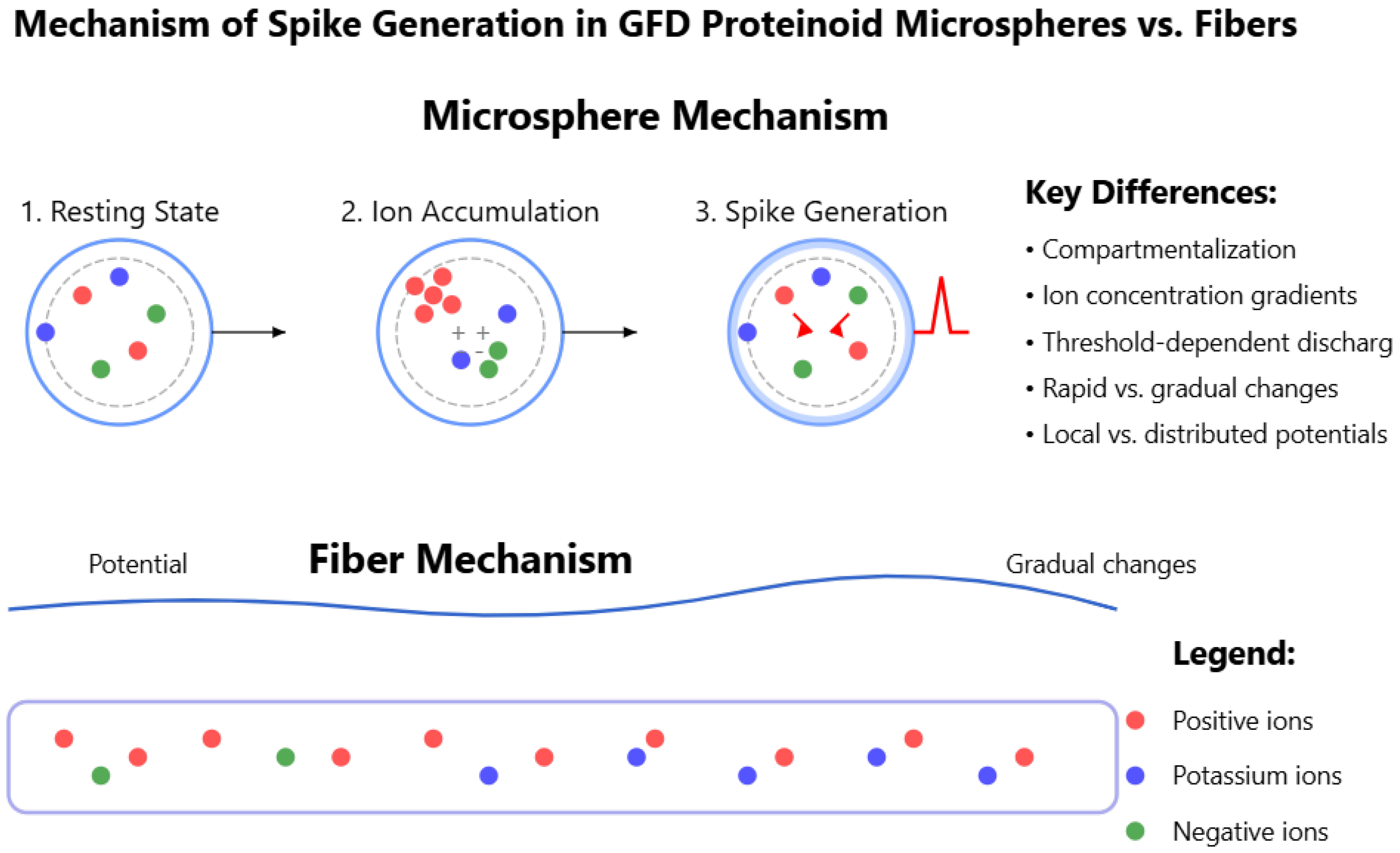
Diagram showing how spike generation works in Glu–Phe–Asp (GFD) proteinoid microspheres and fibers, highlighting how their shapes affect their electrical behavior. The microsphere mechanism has three stages: the resting state, where ions are balanced; ion accumulation, which creates concentration gradients; and spike generation, where a threshold triggers discharge. The fiber mechanism shows gradual potential changes due to distributed ion movement. The key differences are compartmentalization, ion gradients, rapid versus gradual changes, and local versus distributed potentials. Positive ions are shown in red, potassium ions in blue, and negative ions in green. This matches the quick spikes seen in
Figure 6 and the slow waves in
Figure 8, demonstrating how structure affects GFD network dynamics.
Figure 17.
Diagram showing how spike generation works in Glu–Phe–Asp (GFD) proteinoid microspheres and fibers, highlighting how their shapes affect their electrical behavior. The microsphere mechanism has three stages: the resting state, where ions are balanced; ion accumulation, which creates concentration gradients; and spike generation, where a threshold triggers discharge. The fiber mechanism shows gradual potential changes due to distributed ion movement. The key differences are compartmentalization, ion gradients, rapid versus gradual changes, and local versus distributed potentials. Positive ions are shown in red, potassium ions in blue, and negative ions in green. This matches the quick spikes seen in
Figure 6 and the slow waves in
Figure 8, demonstrating how structure affects GFD network dynamics.
Table 1.
Representative examples of protein polymorphism across structural and functional categories.
Table 1.
Representative examples of protein polymorphism across structural and functional categories.
| Protein Type | Polymorphic Structures | Functional Implications |
|---|
| Amyloidogenic Proteins [19] | Soluble monomers, oligomers, protofibrils, mature fibrils | Transition from physiological function to pathological aggregates in neurodegenerative disorders (Alzheimer’s, Parkinson’s) |
| Prion Proteins [20] | (cellular form), (scrapie form) | Conformational change from predominantly -helical to -sheet rich structure leads to infectious propagation and neurodegeneration |
| Hemoglobin [21] | Tense (T) state, relaxed (R) state | Allosteric regulation of oxygen binding affinity through quaternary structural transitions |
| Heat Shock Proteins [22] | Monomeric, oligomeric, and substrate-bound forms | Chaperone activity modulated by dynamic assembly/disassembly in response to cellular stress conditions |
| Crystallins [23] | Soluble oligomers, insoluble aggregates, amorphous deposits | Age-related transition from transparent lens proteins to cataract-forming structures |
| Viral Capsid Proteins [24] | Pentameric assemblies, hexameric assemblies, mature capsid | Structural transitions essential for viral assembly, maturation, and host cell interaction |
| Proteinoids [this work] | Microspheres, fibers, mixed morphologies | Self-assembly into distinct structures with differential electrical properties and information processing capabilities |
| Intrinsically Disordered Proteins [25] | Extended random coils, partially structured intermediates, folded states | Functional plasticity enabling interactions with multiple binding partners in signaling pathways |
| G-Protein Coupled Receptors [26] | Inactive conformation, active conformation, various intermediate states | Conformational selection determines signaling outcomes in response to different ligands |
| Tubulin [27] | / heterodimers, protofilaments, microtubules, sheets | Dynamic instability and structural transitions essential for cellular division and intracellular transport |
Table 2.
Key Raman spectral features for Glu-Phe-Asp proteinoid morphologies. Fibers exhibit numerous sharp, well-defined peaks throughout the spectrum, particularly at 1000 cm−1 (strong, narrow peak) and 1250 cm−1 (amide III), indicating high molecular order. In contrast, microspheres show a smooth profile with minimal distinct peaks and a broad, continuous decline from 500–2000 cm−1, suggesting molecular disorder. The fiber+microsphere mixture displays intermediate characteristics with some defined features at 750 cm−1 and 1250 cm−1 superimposed on a rising baseline.
| Morphology | Key Spectral Features | Structural Implications |
|---|
| Fibers | Multiple sharp peaks (250–1750 cm−1)
Prominent peaks at ∼500, 650, 1000, 1250, 1650 cm−1
Sharp, high-intensity peak at 1000 cm−1 | High degree of molecular order
Consistent inter-chain interactions
Aligned aromatic (Phe) residues
Directional hydrogen bonding |
| Microspheres | Smooth spectral profile
Broad peak at ∼350 cm−1
Continuous intensity decline from 500–2000 cm−1
Minimal distinct features at 1250, 1650 cm−1 | Significant molecular disorder
Heterogeneous molecular arrangement
Isotropic self-assembly
Random orientation of side chains |
| Fibers + Microspheres | Intermediate spectral profile
Step-like increase at ∼750 cm−1
Subtle features at 1250, 1650 cm−1
Rising baseline beyond 1700 cm−1 | Combined structural elements
Dominated by microsphere contributions
Mixed ordered/disordered regions
Complex interfacial interactions |
Table 3.
Detailed statistics of impedance (Z/Ohm), capacitance (Cs/F), and resistance (Idc/m) for GFD proteinoid samples over 1000 s, derived from time-series data.
Table 3.
Detailed statistics of impedance (Z/Ohm), capacitance (Cs/F), and resistance (Idc/m) for GFD proteinoid samples over 1000 s, derived from time-series data.
| | Impedance (Z/Ohm) | Capacitance (Cs/F) | Resistance (Idc/m) |
|---|
| Sample | Mean | Std | Min | Max | Median | Mean | Std | Min | Max | Median | Mean | Std | Min | Max | Median | Slope |
|---|
| Fibers | 209.400 | 0.286 | 208.349 | 210.225 | 209.401 | 9.912 | 0.171 | 9.436 | 10.434 | 9.898 | 163,067.613 | 9253.064 | 157,464.172 | 212,725.067 | 159,023.422 | −26.613 |
| Mixture | 404.235 | 1.091 | 400.544 | 408.045 | 404.226 | 3.328 | 0.076 | 3.062 | 3.601 | 3.326 | 60,424.487 | 1293.986 | 59,054.138 | 67,298.653 | 59,998.276 | −4.707 |
| Microspheres | 6646.282 | 178.664 | 6346.610 | 7038.241 | 6620.197 | 1.926 | 5.735 | 0.633 | 162.514 | 1.452 | 15,830.739 | 652.514 | 14,643.011 | 18,024.274 | 16,000.094 | −2.483 |


