
A Novel Black Widow Optimization Algorithm Based on Lagrange Interpolation Operator for ResNet18

 ,
,
Abstract
1. Introduction
2. Related Theoretical Description
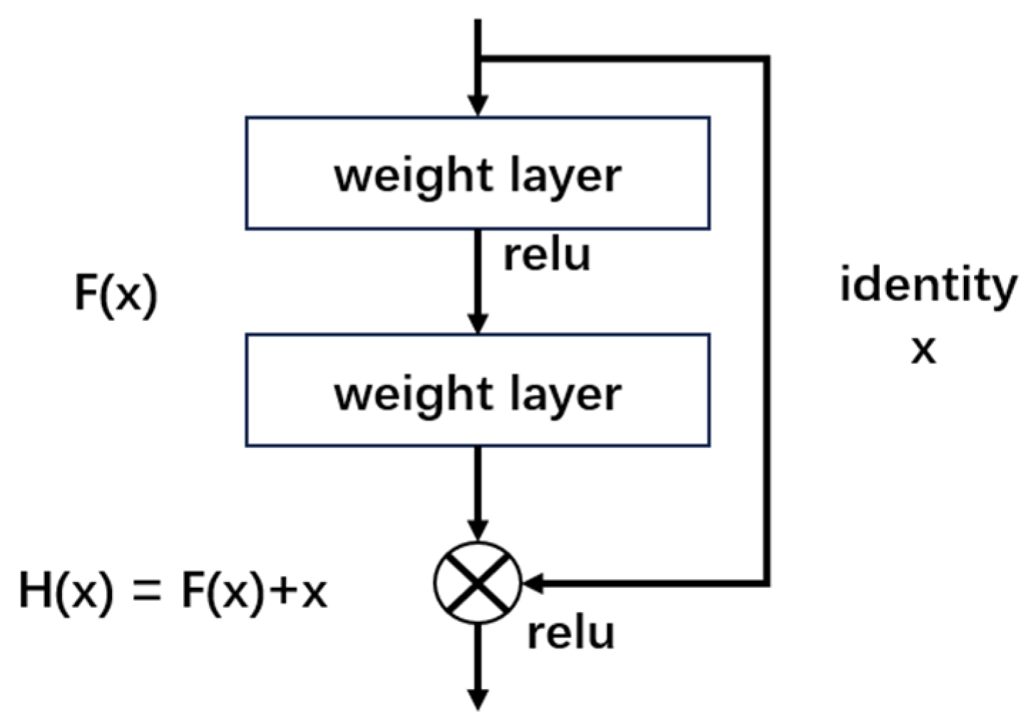
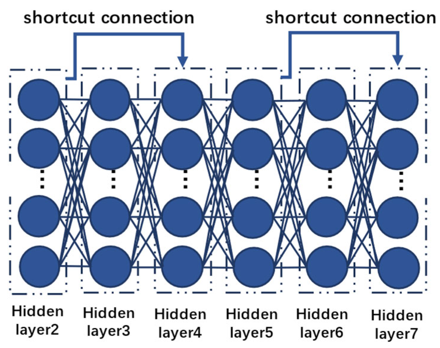
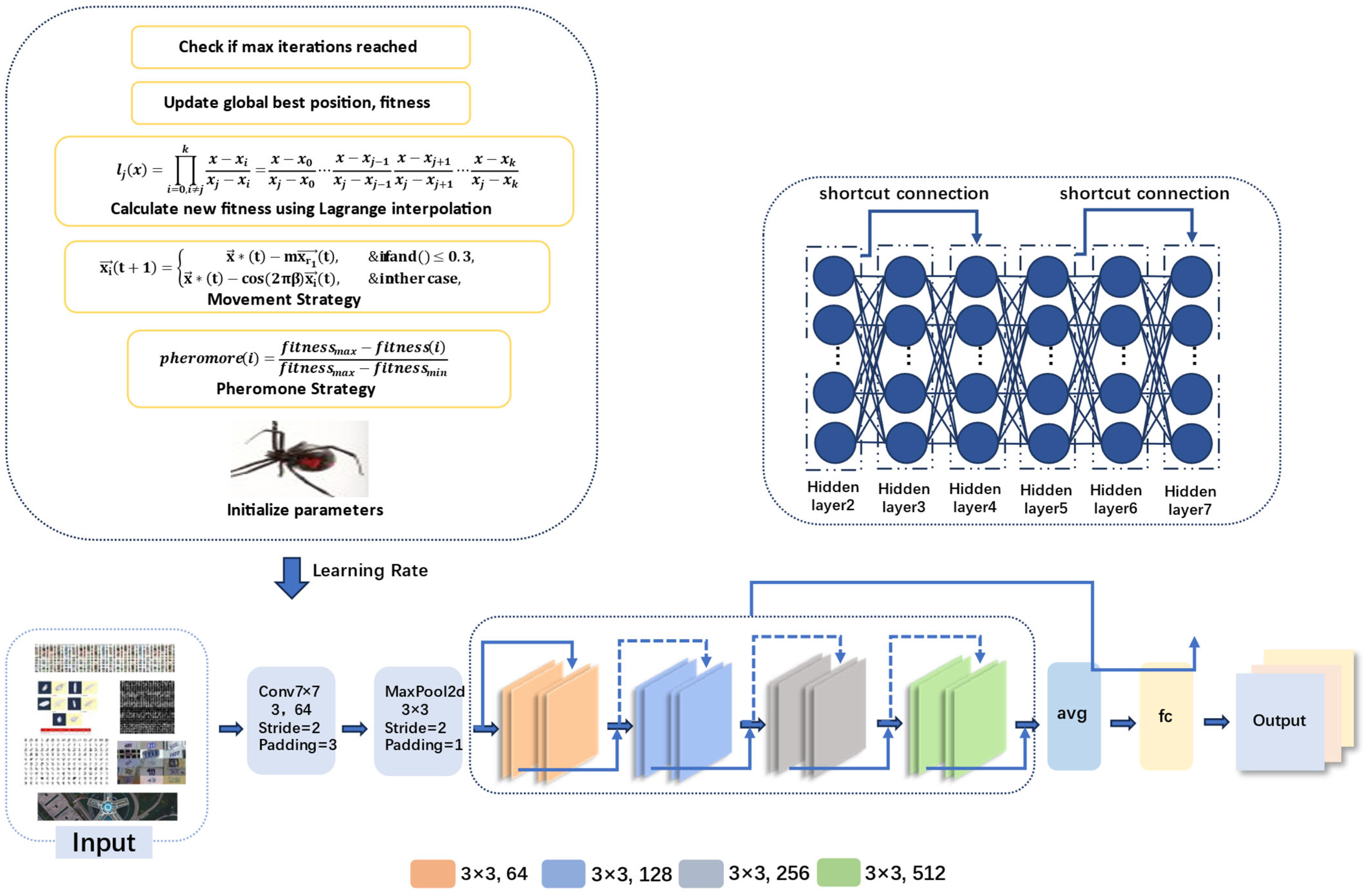
2.1. ResNet18 Model
2.2. Black Widow Optimization Algorithm
- Movement Strategy
- 2.
- Pheromone
| Algorithm 1: BWO | ||
| Input: MaxIter, pop, dim | ||
| Operation | ||
| /* Initialization */ | ||
| 1. | Initialize: MaxIter, pop, dim | |
| 2. | Initialize: parameters m and | |
| /* Training Starts */ | ||
| 3. | while iteration < Max Number of Iterations do | |
| 4. | if random < 0.3 then | |
| 5. 6. 7. 8. 9. 10. 11. 12. 13. 14. 15. | else end if Calculate the pheromone for each search agent using the specified Equation (6) Revise search agents with low pheromone values using its Equation (7) Calculate fitness value of the new search agents if then end if | |
| 16. | end while | |
| /* Operation Ending */ | ||
| Output: , the best optimal solution | ||
2.3. Lagrange Interpolation Method
- Determining the coordinate information of the three known points.
- 2.
- Calculating the Lagrange basis function.
- 3.
- The Lagrange interpolation polynomial is obtained by adding three equations together.
2.4. The Model Design Based on the LIBWONN Method
| Algorithm 2: LIBWONN | ||
| Input: MaxIter, pop, dim | ||
| Operation | ||
| /* Initialization */ | ||
| 1. | Initialize: MaxIter, pop, dim | |
| 2. | Initialize: parameters m and | |
| /* Training Starts */ | ||
| 3. | while iteration < Max Number of Iterations do | |
| 4. | if random < 0.3 then | |
| 5. 6. 7. 8. 9. 10. 11. 12. 13. 14. 15. 16. 17. 18. 19. | else end if Calculate the pheromone for each search agent using the specified Equation (6) Revise search agents with low pheromone values using its Equation (7) Calculate fitness value of the new search agents if then end if if then end if | |
| 20. | end while | |
| /* Operation Ending */ | ||
| Output: , the best optimal solution | ||
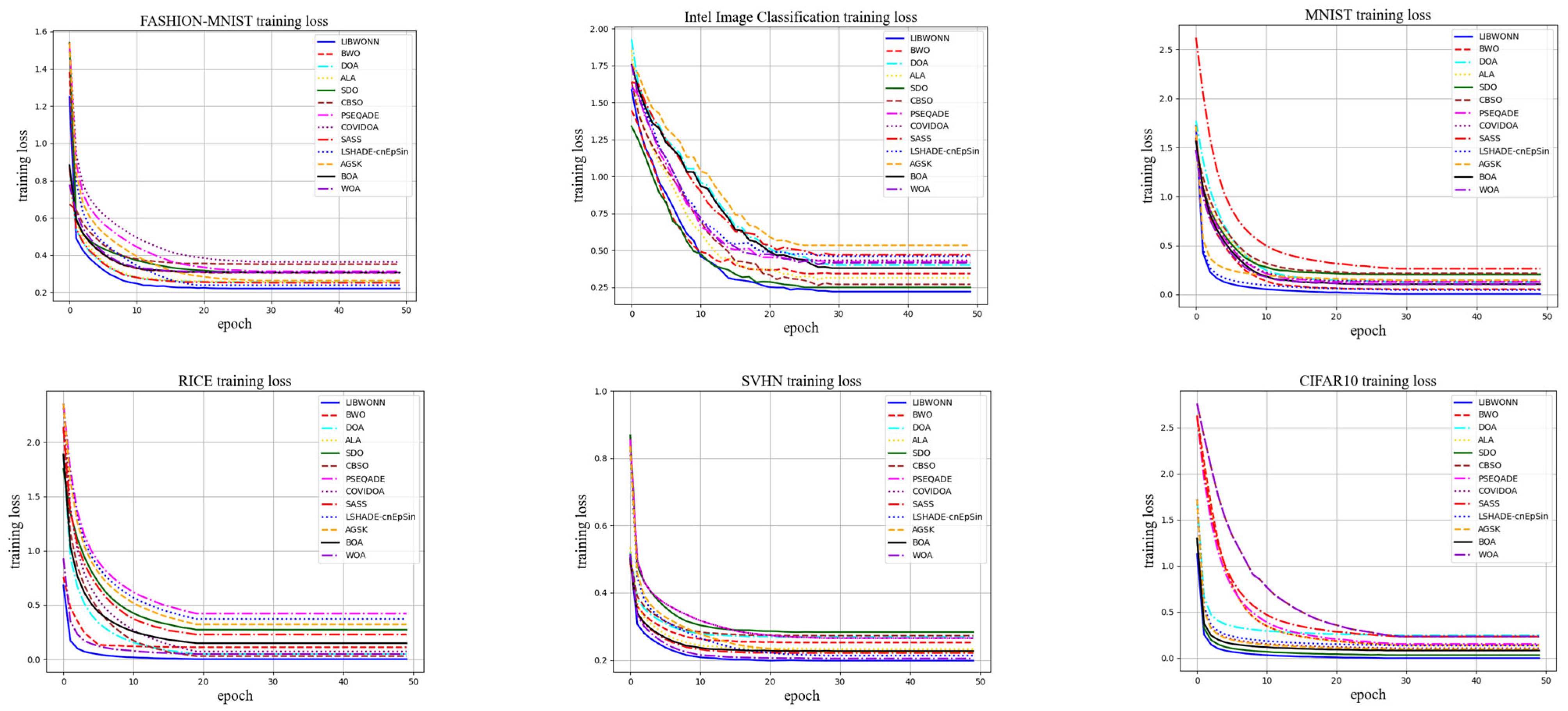
3. Experiments and Analyses
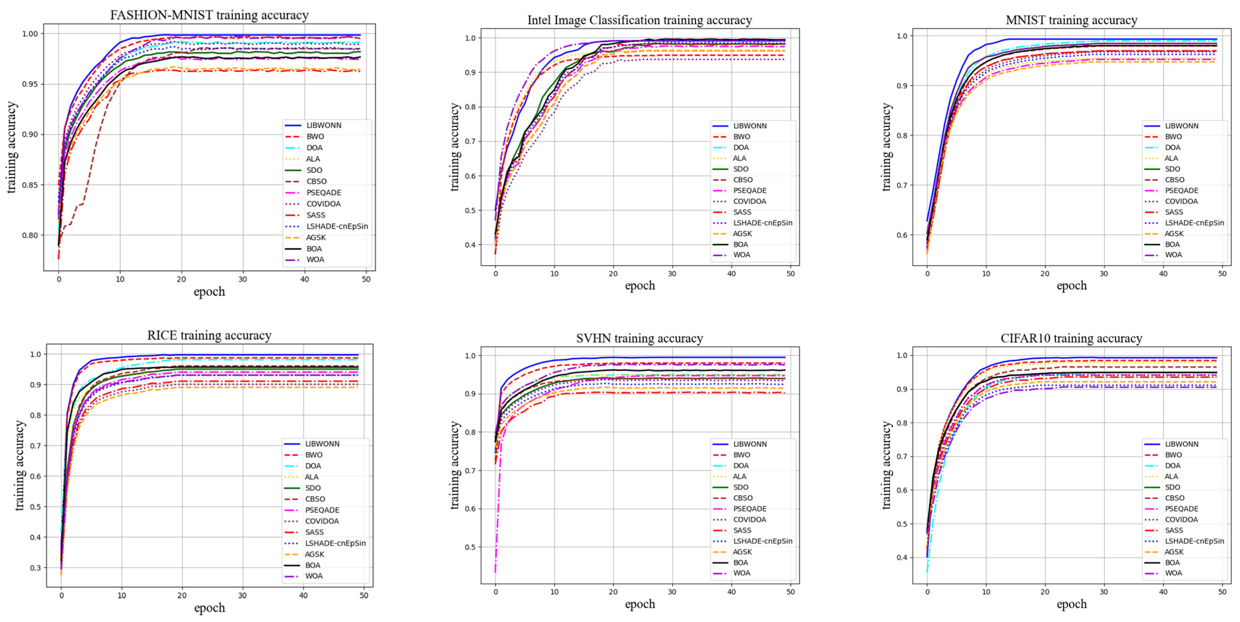
3.1. Dataset
- FASHION-MNIST [52]: A clothing image dataset with grayscale images sized 28 × 28 pixels contains 10 different clothing categories, such as T-shirts, trousers, dresses. The training set contains 60,000 samples, while the test set comprises 10,000 samples.
- MNIST [53]: This dataset for handwritten digit recognition contains 28 × 28 pixel images of digits from 0 to 9, with 60,000 samples for training and 10,000 samples for testing.
- Intel Image Classification [54]: This dataset includes images from six different categories, like buildings, forests, glaciers, mountains, oceans, and cities. All images are standardized to 150 × 150 pixels. The training set contains 14,034 samples, and the testing set has 3,000 samples.
- SVHN [55]: A digit recognition dataset has street-view images with 32 × 32 pixels. It includes 10 categories corresponding to the digits 0–9, and has 73,254 training images and 26,032 test images.
- RICE [56]: It covers five common rice varieties: Arborio, Basmati, Ipsala, Jasmine, and Karacadag. Image dimensions are 224 × 224 pixels with a total of 3,800 images.
- CIFAR10 [57]: This dataset includes images from 10 different categories: Airplane, automobile, bird, cat, deer, dog, frog, horse, ship, and truck. The images are 32 × 32 pixels with a training set of 50,000 images and a test set of 10,000 images.
3.2. Base Models
- DOA: Dream Optimization Algorithm (DOA) is a novel metaheuristic algorithm inspired by human dreams. The algorithm combines a basic memory strategy with a forgetting and replenishing strategy to balance exploration and exploitation.
- ALA: Artificial Lemming Algorithm (ALA) is a biologically inspired metaheuristic algorithm inspired by the four basic behaviors of lemmings in nature: long migrations, digging holes, foraging for food, and avoiding predators. The algorithm simulates the survival strategies of lemmings in complex environments, providing an effective search method for solving optimization problems.
- SDO: Sled Dog Optimizer (SDO) is mainly inspired by the various behavior patterns of sled dogs, focusing on simulating the processes of dogs pulling sleds, training, and retiring to construct a mathematical model.
- CBSO: Connected Banking System Optimizer (CBSO) is a population-based optimization algorithm that belongs to a multi-stage search strategy. It is inspired by the interconnectedness of banking systems, where different banks are connected in various ways, facilitating transactions and submissions.
- PSEQADE: Quantum Adaptive Population State Evaluation Differential Evolution Algorithm (PSEQADE) is an improved quantum heuristic differential evolution algorithm. It adopts a quantum adaptive mutation strategy to reduce excessive mutation and introduces a population state evaluation framework to enhance convergence accuracy and stability.
- COVIDOA: Coronavirus Optimization Algorithm (COVIDOA) is an evolutionary algorithm that simulates the biological lifecycle. It is inspired by the behavior of organisms at different stages such as growth, reproduction, and adaptation. The algorithm simulates the evolutionary process of individuals from youth to adulthood, adapting through mutation, recombination, selection, and reproduction based on environmental changes, thereby balancing global and local search capabilities.
- SASS: Social-Aware Salp Swarm Algorithm (SASS) is a population-based optimization algorithm inspired by the behavior of sand particles in a sandstorm. It mainly simulates the collective movement of sand particles under the influence of wind to perform global optimization. The goal of SASS is to improve collaboration among individuals in the group using a social awareness model, enhancing the balance between exploration and exploitation in the search process.
- LSHADE-cnEpSin: Latent Search Strategy Adaptive Differential Evolution with Compound Neighborhood-based Epistemic Population for Sine Function (LSHADE-cnEpSin) is an improved differential evolution algorithm. It enhances optimization performance, especially for high-dimensional complex problems, by using an adaptive mutation strategy and a control mechanism that balances global and local search.
- AGSK: Adaptive Gaining Sharing Knowledge (AGSK) is an algorithm that simulates the human knowledge-sharing process. It enhances global search capability and local search efficiency by introducing an adaptation strategy based on successful historical positional information, making it suitable for solving complex optimization problems.
- BOA: The Bobcat Optimization Algorithm (BOA) is a bio-inspired metaheuristic algorithm that simulates the natural hunting behavior of bobcats. It enhances the balance between global exploration and local exploitation by modeling two phases: the bobcat’s movement towards its prey (exploration) and the chase process to catch its prey (exploitation). BOA’s dual-phase position update strategy improves convergence speed and solution quality, making it effective for solving high-dimensional, complex, and constrained optimization problems.
- WOA: The Wombat Optimization Algorithm (WOA) is a bio-inspired metaheuristic algorithm that simulates the foraging behavior of wild wombats and their evasive maneuvers against predators. The algorithm models two phases: the wombat’s position changes during foraging (exploration) and its movements when diving into tunnels to escape predators (exploitation), effectively balancing global search and local search.
3.3. Performance Verification
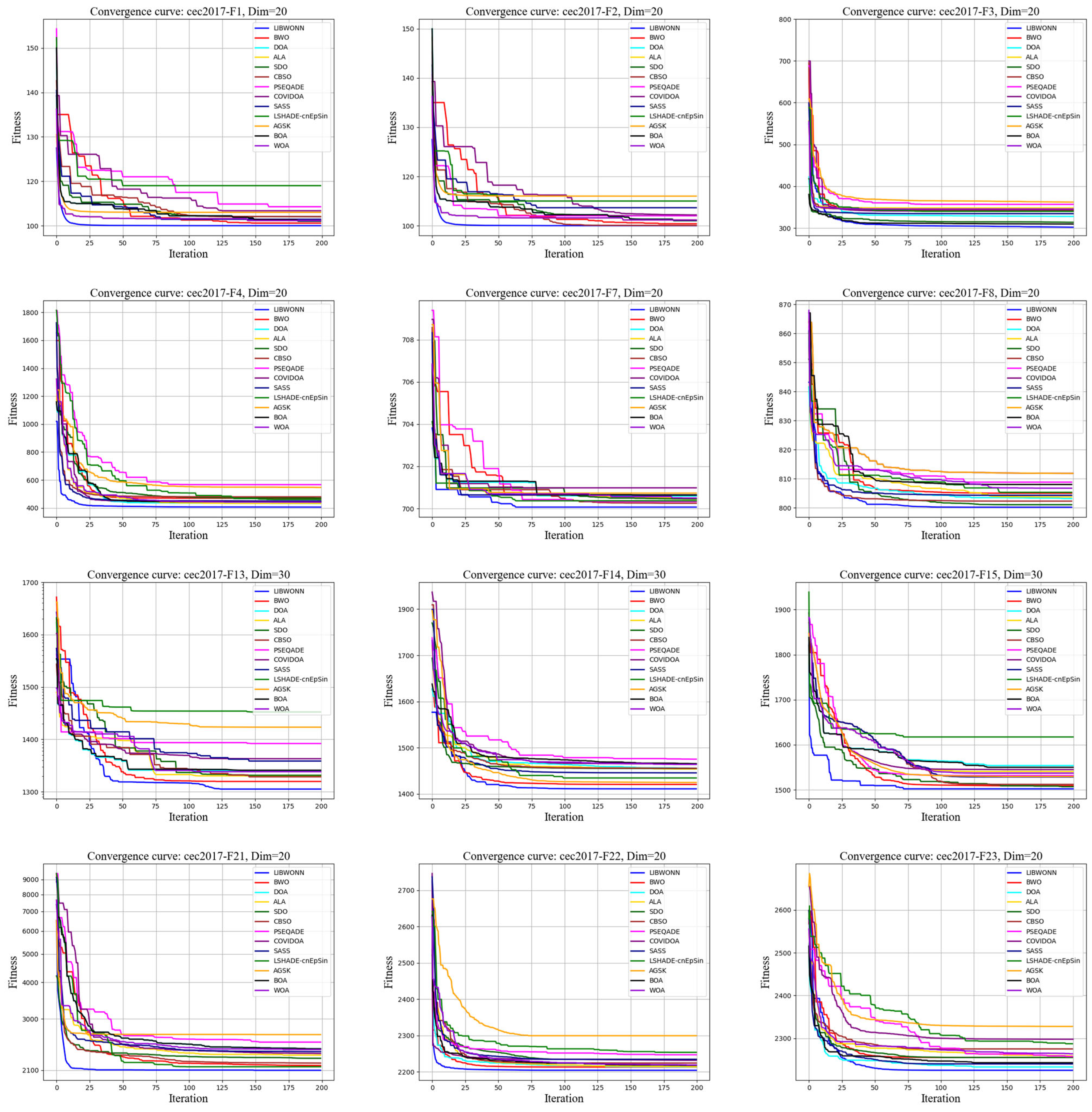
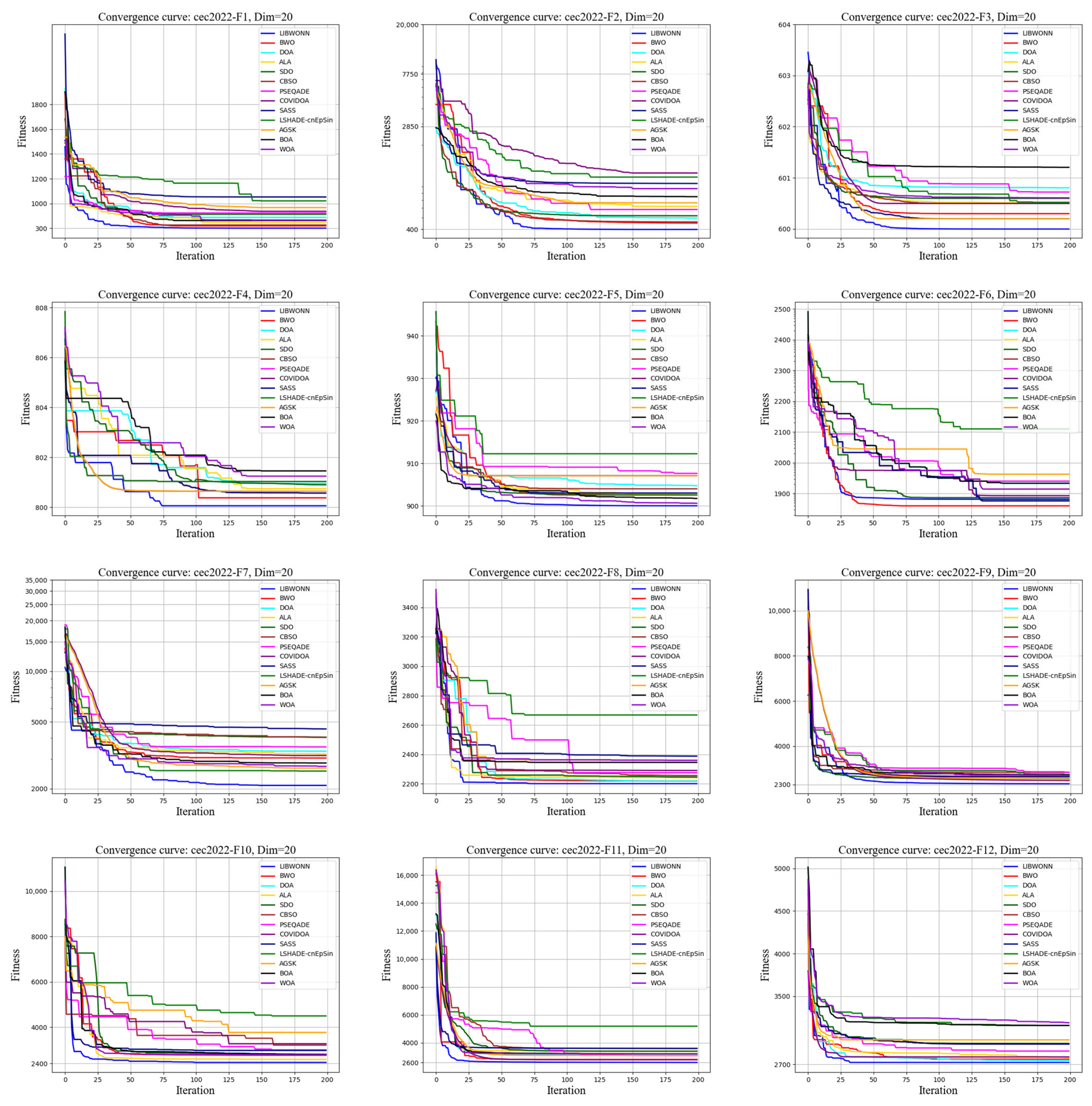
3.4. Testing Functions
- Unimodal functions: Characterized by a single global optimum, they are used to test an algorithm’s local search proficiency and convergence speed. They are effective in evaluating the algorithm’s efficiency and accuracy in basic situations.
- Multimodal functions: Characterized by several local optima, they test the performance of an algorithm to navigate out of local optima as well as its global search capability. These functions are adopted to measure the performance of the algorithm in complex and nonlinear environments.
- Composite functions: They are composed of multiple functions with different characteristics, which simulate the complexity and diversity of real-world problems. They are adopted to verify the algorithm’s adaptability when handling mixed features and multiple levels of difficulty.
- Dynamic change functions: Their objective function changes over time, and are used to evaluate the algorithm’s tracking and adaptability in dynamic environments. They are especially suitable for testing an algorithm’s ability to maintain its performance under continuously changing conditions.
- Average value (Ave):
- 2.
- Best value (Best):
- 3.
- Standard deviation (Std):
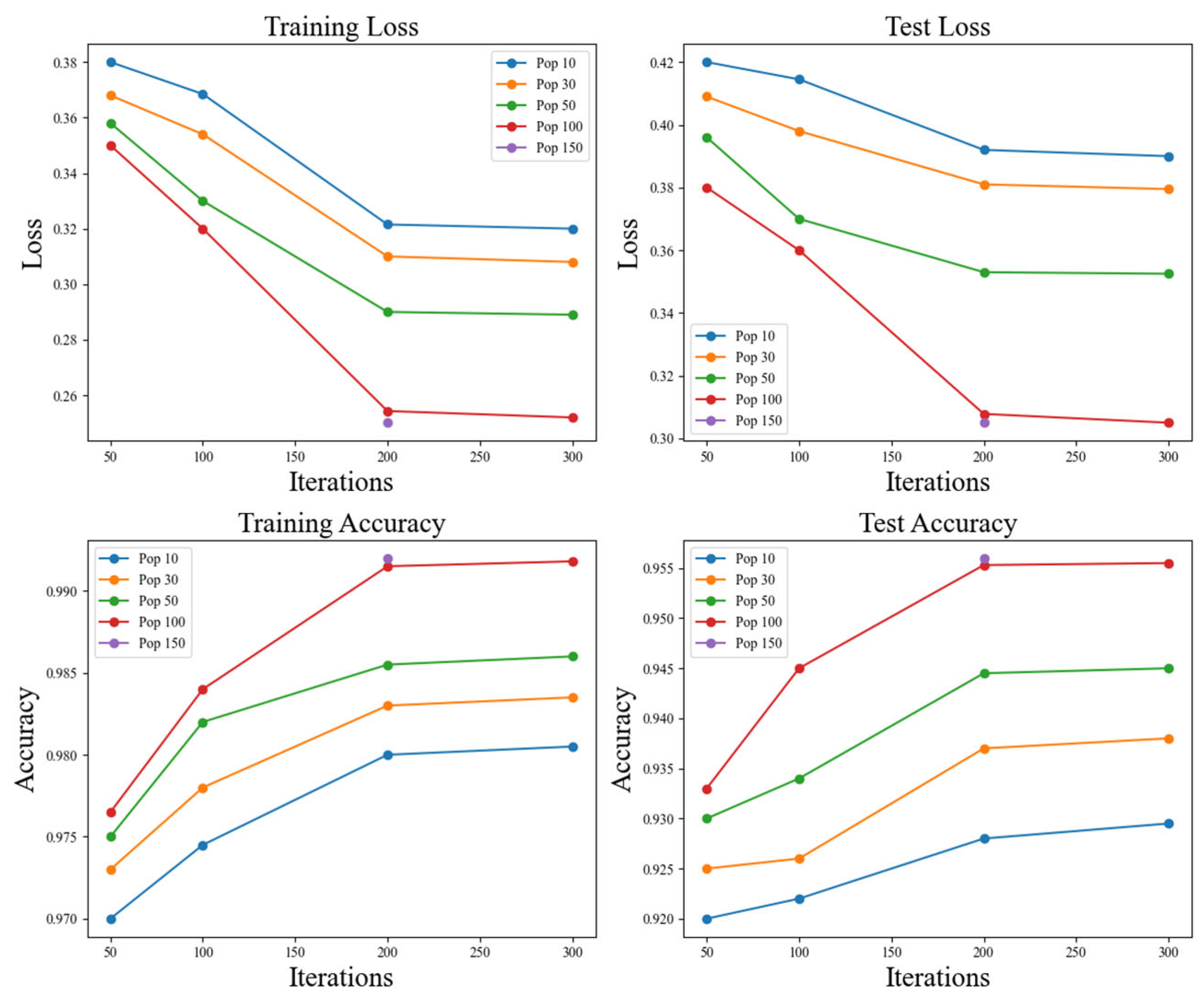
3.5. Ablation Study and Sensitivity Analysis
4. Conclusions
Author Contributions
Funding
Institutional Review Board Statement
Informed Consent Statement
Data Availability Statement
Conflicts of Interest
References
- Yuan, J.; Zhu, A.; Xu, Q.; Wattanachote, K.; Gong, Y. CTIF-Net: A CNN-transformer iterative fusion network for salient object detection. IEEE Trans. Circuits Syst. Video Technol. 2024, 34, 3795–3805. [Google Scholar] [CrossRef]
- He, K.; Zhang, X.; Ren, S.; Sun, R. Deep residual learning for image recognition. In Proceedings of the IEEE Conference on Computer Vision and Pattern Recognition, Las Vegas, NV, USA, 27–30 June 2016; pp. 770–778. [Google Scholar]
- Xu, W.; Fu, Y.-L.; Zhu, D. ResNet and its application to medical image processing: Research progress and challenges. Comput. Methods Programs Biomed. 2023, 240, 107660. [Google Scholar] [CrossRef] [PubMed]
- Croitoru, F.-A.; Ristea, N.-C.; Ionescu, R.T.; Sebe, N. Learning rate curriculum. Int. J. Comput. Vis. 2024, 132, 1–24. [Google Scholar] [CrossRef]
- Razavi, M.; Mavaddati, S.; Koohi, H. ResNet deep models and transfer learning technique for classification and quality detection of rice cultivars. Expert Syst. Appl. 2024, 247, 123276. [Google Scholar] [CrossRef]
- Peña-Delgado, A.F.; Peraza-Vázquez, H.; Almazán-Covarrubias, J.H.; Cruz, N.T.; García-Vite, P.M.; Morales-Cepeda, A.B.; Ramirez-Arredondo, J.M. A Novel bio-inspired algorithm applied to selective harmonic elimination in a three-phase eleven-level inverter. Math. Probl. Eng. 2020, 2020, 8856040. [Google Scholar] [CrossRef]
- Sauer, T.; Xu, Y. On multivariate Lagrange interpolation. Math. Comput. 1995, 64, 1147–1170. [Google Scholar] [CrossRef]
- Ma, Z.; Mao, Z.; Shen, J. Efficient and stable SAV-based methods for gradient flows arising from deep learning. J. Comput. Phys. 2024, 505, 112911. [Google Scholar] [CrossRef]
- Franchini, G.; Porta, F.; Ruggiero, V.; Trombini, I.; Zanni, L. A Stochastic gradient method with variance control and variable learning rate for deep learning. J. Comput. Appl. Math. 2024, 451, 116083. [Google Scholar] [CrossRef]
- Wang, Z.; Zhang, J. Incremental PID controller-based learning rate scheduler for stochastic gradient descent. IEEE Trans. Neural Netw. Learn. Syst. 2024, 35, 7060–7071. [Google Scholar] [CrossRef]
- Qin, W.; Luo, X.; Zhou, M.C. Adaptively-accelerated parallel stochastic gradient descent for high-dimensional and incomplete data representation learning. IEEE Trans. Big Data 2024, 10, 92–107. [Google Scholar] [CrossRef]
- Shen, L.; Chen, C.; Zou, F.; Jie, Z.; Sun, J.; Liu, W. A unified analysis of AdaGrad with weighted aggregation and momentum acceleration. IEEE Trans. Neural Netw. Learn. Syst. 2024, 35, 14482–14490. [Google Scholar] [CrossRef] [PubMed]
- Shao, Y.; Yang, J.; Zhou, W.; Sun, H.; Xing, L.; Zhao, Q.; Zhang, L. An improvement of adam based on a cyclic exponential decay learning rate and gradient norm constraints. Electronics 2024, 13, 1778. [Google Scholar] [CrossRef]
- Jia, X.; Feng, X.; Yong, H.; Meng, D. Weight decay with tailored adam on scale-invariant weights for better generalization. IEEE Trans. Neural Netw. Learn. Syst. 2024, 35, 6936–6947. [Google Scholar] [CrossRef] [PubMed]
- Wilson, A.C.; Roelofs, R.; Stern, M.; Srebro, N.; Recht, B. The marginal value of adaptive gradient methods in machine learning. Proc. Adv. Neural Inf. Process. Syst. 2017, 30, 4149–4159. [Google Scholar]
- Gharehchopogh, F.S. Quantum-inspired metaheuristic algorithms: Comprehensive survey and classification. Artif. Intell. Rev. 2023, 56, 5479–5543. [Google Scholar] [CrossRef]
- Akgul, A.; Karaca, Y.; Pala, M.A.; Çimen, M.E.; Boz, A.F.; Yildiz, M.Z. Chaos theory, advanced metaheuristic algorithms and their newfangled deep learning architecture optimization applications: A review. Fractals 2024, 32, 2430001. [Google Scholar] [CrossRef]
- Wang, X.; Hu, H.; Liang, Y.; Zhou, L. On the mathematical models and applications of swarm intelligent optimization algorithms. Arch. Comput. Methods Eng. 2022, 29, 3815–3842. [Google Scholar] [CrossRef]
- Li, J.; Yang, S.X. Intelligent fish-inspired foraging of swarm robots with sub-group behaviors based on neurodynamic models. Biomimetics 2024, 9, 16. [Google Scholar] [CrossRef]
- Chen, B.; Cao, L.; Chen, C.; Chen, Y.; Yue, Y. A comprehensive survey on the chicken swarm optimization algorithm and its applications: State-of-the-art and research challenges. Artif. Intell. Rev. 2024, 57, 170. [Google Scholar] [CrossRef]
- Deng, W.; Ma, X.; Qiao, W. A hybrid intelligent optimization algorithm based on a learning strategy. Mathematics 2024, 12, 2570. [Google Scholar] [CrossRef]
- Guan, T.; Wen, T.; Kou, B. Improved lion swarm optimization algorithm to solve the multi-objective rescheduling of hybrid flowshop with limited buffer. J. King Saud Univ.-Comput. Inf. Sci. 2024, 36, 102077. [Google Scholar] [CrossRef]
- Xu, Y.; Zhang, M.; Yang, M.; Wang, D. Hybrid quantum particle swarm optimization and variable neighborhood search for flexible job-shop scheduling problem. J. Manuf. Syst. 2024, 73, 334–348. [Google Scholar] [CrossRef]
- Zhong, M.; Wen, J.; Ma, J.; Cui, H.; Zhang, Q.; Parizi, M.K. A hierarchical multi-leadership sine cosine algorithm to dissolving global optimization and data classification: The COVID-19 case study. Comput. Biol. Med. 2023, 164, 107212. [Google Scholar] [CrossRef]
- Mohamed, M.T.; Alkhalaf, S.; Senjyu, T.; Mohamed, T.H.; Elnoby, A.M.; Hemeida, A. Sine cosine optimization algorithm combined with balloon effect for adaptive position control of a cart forced by an armature-controlled DC motor. PLoS ONE 2024, 19, e0300645. [Google Scholar] [CrossRef]
- Miao, F.; Wu, Y.; Yan, G.; Si, X. A memory interaction quadratic interpolation whale optimization algorithm based on reverse information correction for high-dimensional feature selection. Appl. Soft Comput. 2024, 164, 111979. [Google Scholar] [CrossRef]
- Wei, P.; Shang, M.; Zhou, J.; Shi, X. Efficient adaptive learning rate for convolutional neural network based on quadratic interpolation egret swarm optimization algorithm. Heliyon 2024, 10, e37814. [Google Scholar] [CrossRef]
- Deng, W.; Wang, J.; Guo, A.; Zhao, H. Quantum differential evolutionary algorithm with quantum-adaptive mutation strategy and population state evaluation framework for high-dimensional problems. Inf. Sci. 2024, 676, 120787. [Google Scholar] [CrossRef]
- Khalid, A.M.; Hosny, K.M.; Mirjalili, S. COVIDOA: A novel evolutionary optimization algorithm based on coronavirus disease replication lifecycle. Neural Comput. Appl. 2022, 34, 22465–22492. [Google Scholar] [CrossRef]
- Salgotra, R.; Singh, U.; Saha, S.; Nagar, A. New Improved SALSHADE-cnEpSin Algorithm with Adaptive Parameters. IEEE Congr. Evol. Comput. (CEC) 2019, 2019, 3150–3156. [Google Scholar]
- Xiao, Y.; Cui, H.; Abu Khurma, R.; Castillo, P.A. Artificial lemming algorithm: A novel bionic meta-heuristic technique for solving real-world engineering optimization problems. Artif. Intell. Rev. 2025, 58, 84. [Google Scholar] [CrossRef]
- Hu, G.; Cheng, M.; Houssein, E.H.; Hussien, A.G.; Abualigah, L. SDO: A novel sled dog-inspired optimizer for solving engineering problems. Adv. Eng. Inform. 2024, 62, 102783. [Google Scholar] [CrossRef]
- Rao, A.N.; Vijayapriya, P. Salp Swarm Algorithm and Phasor Measurement Unit Based Hybrid Robust Neural Network Model for Online Monitoring of Voltage Stability. Wirel. Netw. 2021, 27, 843–860. [Google Scholar]
- Benmamoun, Z.; Khlie, K.; Bektemyssova, G.; Dehghani, M.; Gherabi, Y. Bobcat Optimization Algorithm: An effective bio-inspired metaheuristic algorithm for solving supply chain optimization problems. Sci. Rep. 2024, 14, 20099. [Google Scholar] [CrossRef]
- Benmamoun, Z.; Khlie, K.; Dehghani, M.; Gherabi, Y. WOA: Wombat optimization algorithm for solving supply chain optimization problems. Mathematics 2024, 12, 1059. [Google Scholar] [CrossRef]
- Lang, Y.; Gao, Y. Dream Optimization Algorithm (DOA): A novel metaheuristic optimization algorithm inspired by human dreams and its applications to real-world engineering problems. Comput. Methods Appl. Mech. Eng. 2025, 436, 117718. [Google Scholar] [CrossRef]
- Nemati, M.; Zandi, Y.; Sabouri, J. Application of a novel metaheuristic algorithm inspired by connected banking system in truss size and layout optimum design problems and optimization problems. Sci. Rep. 2024, 14, 27345. [Google Scholar] [CrossRef]
- Akhmedova, S.; Stanovov, V. Success-History Based Position Adaptation in Gaining-Sharing Knowledge Based Algorithm. In Proceedings of the Advances in Swarm Intelligence: 12th International Conference, Qingdao, China, 17–21 July 2021; Volume 12, pp. 174–181. [Google Scholar]
- Beheshti, Z.; Shamsuddin, S.M.H. A review of population-based meta-heuristic algorithms. Int. J. Adv. Soft. Comput. Appl. 2013, 5, 1–35. [Google Scholar]
- Wang, J.; Liang, Y.; Tang, J.; Wu, Z. Vehicle trajectory reconstruction using lagrange-interpolation-based framework. Appl. Sci. 2024, 14, 1173. [Google Scholar] [CrossRef]
- Wang, R.; Feng, Q.; Ji, J. The discrete convolution for fractional cosine-sine series and its application in convolution equations. AIMS Math. 2024, 9, 2641–2656. [Google Scholar] [CrossRef]
- Taylor, R.L. Newton interpolation. Numer. Anal. 2022, 12, 25–37. [Google Scholar]
- Smith, M.J. Spline interpolation. J. Comput. Math. 2021, 18, 58–72. [Google Scholar]
- Thompson, A.P. Quadratic interpolation: Formula, definition, and solved examples. Appl. Math. Comput. 2023, 20, 65–78. [Google Scholar]
- Acton, F.S. Linear vs. quadratic interpolations example from F.S. Acton ‘Numerical methods that work’. Numer. Methods J. 2020, 9, 101–110. [Google Scholar]
- Zhang, X. Research on interpolation and data fitting: Basis and applications. Math. Model. Appl. 2022, 35, 125–135. [Google Scholar]
- Bengio, Y.; Simard, P.; Frasconi, P. Learning long-term dependencies with gradient descent is difficult. Neural Comput. 1994, 6, 157–167. [Google Scholar] [CrossRef]
- Hochreiter, S.; Schmidhuber, J. Long short-term memory. Neural Comput. 1997, 9, 1735–1780. [Google Scholar] [CrossRef]
- Goodfellow, I.J.; Pouget-Abadie, J.; Mirza, M.; Xu, B.; Warde-Farley, D.; Ozair, S.; Courville, A.; Bengio, Y. Generative adversarial nets. In Proceedings of the 27th International Conference on Neural Information Processing Systems (NIPS), Montreal, QC, Canada, 8–13 December 2014; pp. 2672–2680. [Google Scholar]
- Simonyan, K.; Zisserman, A. Very deep convolutional networks for large-scale image recognition. Int. Conf. Mach. Learn. (ICML) 2015, 37, 1–9. [Google Scholar]
- Li, Z.; Li, S.; Luo, X. A novel machine learning system for industrial robot arm calibration. IEEE Trans. Circuits Syst. II Express Briefs 2023, 71, 2364–2368. [Google Scholar] [CrossRef]
- Ma, R.; Hwang, K.; Li, M.; Miao, Y. Trusted model aggregation with zero-knowledge proofs in federated learning. IEEE Trans. Parallel Distrib. Syst. 2024, 35, 2284–2296. [Google Scholar] [CrossRef]
- Tissera, M.D.; McDonnell, M.D. Deep extreme learning machines: Supervised autoencoding architecture for classification. Neurocomputing 2016, 174, 42–49. [Google Scholar] [CrossRef]
- Abhishek, A.V.S.; Gurrala, V.R. Improving model performance and removing the class imbalance problem using augmentation. Technology (IJARET) 2022, 13, 14–22. [Google Scholar]
- Netzer, Y.; Wang, T.; Coates, A.; Bissacco, A.; Wu, B.; Ng, A.Y. Reading digits in natural images with unsupervised feature learning. NIPS Workshop Deep Learn. Unsupervised Feature Learn. 2011, 2011, 4. [Google Scholar]
- Koklu, M.; Cinar, I.; Taspinar, Y.S. Classification of rice varieties with deep learning methods. Comput. Electron. Agric. 2021, 187, 106285. [Google Scholar] [CrossRef]
- Krizhevsky, A.; Hinton, G. Learning Multiple Layers Offeatures from Tiny Images. Master’s Thesis, University of Tront, Toronto, ON, Canada, 2009; pp. 1–60. [Google Scholar]


| Baseline | Training Loss | Test Loss | Training Accuracy | Test Accuracy | Precision | Recall | F1-Score |
|---|---|---|---|---|---|---|---|
| ResNet18 | 0.2610 | 0.3405 | 0.9946 | 0.9533 | 0.95 | 0.95 | 0.95 |
| RNN | 0.3721 | 0.3905 | 0.9703 | 0.9217 | 0.91 | 0.91 | 0.91 |
| CNN | 0.2895 | 0.3197 | 0.9857 | 0.9475 | 0.94 | 0.94 | 0.94 |
| LSTM | 0.3558 | 0.3729 | 0.9769 | 0.9328 | 0.93 | 0.93 | 0.93 |
| GAN | 0.4012 | 0.4156 | 0.9653 | 0.9105 | 0.90 | 0.90 | 0.90 |
| VGG | 0.2716 | 0.3652 | 0.9521 | 0.9549 | 0.92 | 0.92 | 0.92 |
| Baseline | Training Loss | Test Loss | Training Accuracy | Test Accuracy | Precision | Recall | F1-Score |
|---|---|---|---|---|---|---|---|
| Newton | 0.3102 | 0.3421 | 0.9862 | 0.9384 | 0.93 | 0.94 | 0.93 |
| Spline | 0.2905 | 0.3234 | 0.9901 | 0.9463 | 0.94 | 0.94 | 0.94 |
| Quadratic | 0.3257 | 0.3552 | 0.9837 | 0.9243 | 0.92 | 0.92 | 0.92 |
| Linear | 0.2998 | 0.3327 | 0.9874 | 0.9396 | 0.93 | 0.93 | 0.93 |
| Chebyshev | 0.3179 | 0.3481 | 0.9852 | 0.9358 | 0.93 | 0.93 | 0.93 |
| Lagrange | 0.2610 | 0.3405 | 0.9946 | 0.9533 | 0.95 | 0.95 | 0.95 |
| Baseline | Training Loss | Test Loss | Training Accuracy | Test Accuracy | Precision | Recall | F1-Score | p-Value |
|---|---|---|---|---|---|---|---|---|
| LIBWONN | 0.2717 | 0.2964 | 0.9628 | 0.9498 | 0.94 | 0.95 | 0.95 | 1.000 |
| BWO | 0.2867 | 0.3052 | 0.9391 | 0.9430 | 0.94 | 0.93 | 0.94 | 0.0176 |
| DOA | 0.3211 | 0.3194 | 0.9167 | 0.9361 | 0.93 | 0.93 | 0.93 | 0.0263 |
| ALA | 0.2713 | 0.3068 | 0.9197 | 0.9099 | 0.90 | 0.90 | 0.90 | 0.0381 |
| SDO | 0.2910 | 0.3201 | 0.9580 | 0.9398 | 0.93 | 0.94 | 0.93 | 0.0112 |
| CBSO | 0.3083 | 0.3230 | 0.9107 | 0.9243 | 0.92 | 0.92 | 0.92 | 0.2457 |
| PSEQADE | 0.3148 | 0.3169 | 0.9151 | 0.9241 | 0.93 | 0.93 | 0.93 | 0.1953 |
| COVIDOA | 0.2867 | 0.3052 | 0.9391 | 0.9430 | 0.91 | 0.93 | 0.94 | 0.0214 |
| SASS | 0.3007 | 0.3184 | 0.9376 | 0.9412 | 0.93 | 0.94 | 0.93 | 0.0226 |
| LSHADE | 0.3062 | 0.3215 | 0.9124 | 0.9268 | 0.92 | 0.92 | 0.92 | 0.2468 |
| AGSK | 0.3131 | 0.3152 | 0.9165 | 0.9237 | 0.93 | 0.93 | 0.93 | 0.0311 |
| BOA | 0.2648 | 0.3089 | 0.9423 | 0.9426 | 0.93 | 0.92 | 0.93 | 0.1429 |
| WOA | 0.3174 | 0.3146 | 0.9249 | 0.9312 | 0.93 | 0.93 | 0.93 | 0.2048 |
| Baseline | Training Loss | Test Loss | Training Accuracy | Test Accuracy | Precision | Recall | F1-Score | p-Value |
|---|---|---|---|---|---|---|---|---|
| LIBWONN | 0.0994 | 0.0573 | 0.9912 | 0.9926 | 0.99 | 0.99 | 0.99 | 1.0000 |
| BWO | 0.1414 | 0.0721 | 0.9583 | 0.9776 | 0.98 | 0.98 | 0.98 | 0.0231 |
| DOA | 0.4732 | 0.0567 | 0.9873 | 0.9824 | 0.98 | 0.98 | 0.98 | 0.0442 |
| ALA | 0.1345 | 0.0872 | 0.9602 | 0.9729 | 0.97 | 0.97 | 0.97 | 0.0684 |
| SDO | 0.3221 | 0.0936 | 0.9898 | 0.9903 | 0.99 | 0.99 | 0.99 | 0.0012 |
| CBSO | 0.1384 | 0.1801 | 0.9322 | 0.9468 | 0.95 | 0.95 | 0.95 | 0.2350 |
| PSEQADE | 0.1142 | 0.1205 | 0.9558 | 0.9655 | 0.96 | 0.96 | 0.96 | 0.3120 |
| COVIDOA | 0.1164 | 0.1189 | 0.9524 | 0.9625 | 0.95 | 0.95 | 0.95 | 0.0291 |
| SASS | 0.1318 | 0.1768 | 0.9313 | 0.9458 | 0.95 | 0.95 | 0.95 | 0.3980 |
| LSHADE | 0.1117 | 0.1183 | 0.9548 | 0.9648 | 0.96 | 0.96 | 0.96 | 0.0094 |
| AGSK | 0.1152 | 0.1192 | 0.9515 | 0.9614 | 0.95 | 0.95 | 0.95 | 0.0761 |
| BOA | 0.1268 | 0.1017 | 0.9610 | 0.9702 | 0.97 | 0.97 | 0.97 | 0.2658 |
| WOA | 0.1195 | 0.0946 | 0.9635 | 0.9741 | 0.97 | 0.97 | 0.97 | 0.4682 |
| Baseline | Training Loss | Test Loss | Training Accuracy | Test Accuracy | Precision | Recall | F1-Score | p-Value |
|---|---|---|---|---|---|---|---|---|
| LIBWONN | 0.2610 | 0.3405 | 0.9946 | 0.9533 | 0.95 | 0.95 | 0.95 | 1.0000 |
| BWO | 0.3509 | 0.3741 | 0.9738 | 0.9332 | 0.93 | 0.93 | 0.93 | 0.0321 |
| DOA | 0.3981 | 0.4098 | 0.9755 | 0.9245 | 0.93 | 0.92 | 0.92 | 0.0154 |
| ALA | 0.3501 | 0.3714 | 0.9794 | 0.9272 | 0.93 | 0.93 | 0.93 | 0.0468 |
| SDO | 0.3191 | 0.3584 | 0.9760 | 0.9252 | 0.92 | 0.93 | 0.93 | 0.0023 |
| CBSO | 0.2853 | 0.3083 | 0.9612 | 0.9451 | 0.94 | 0.94 | 0.94 | 0.0214 |
| PSEQADE | 0.3271 | 0.3523 | 0.9742 | 0.9162 | 0.91 | 0.91 | 0.91 | 0.1832 |
| COVIDOA | 0.3496 | 0.3597 | 0.9649 | 0.9267 | 0.92 | 0.92 | 0.92 | 0.0587 |
| SASS | 0.2858 | 0.3088 | 0.9604 | 0.9449 | 0.94 | 0.94 | 0.94 | 0.0914 |
| LSHADE | 0.3289 | 0.3537 | 0.9724 | 0.9164 | 0.91 | 0.91 | 0.91 | 0.0009 |
| AGSK | 0.3493 | 0.3586 | 0.9652 | 0.9270 | 0.92 | 0.92 | 0.92 | 0.0275 |
| BOA | 0.3124 | 0.3367 | 0.9688 | 0.9341 | 0.93 | 0.93 | 0.93 | 0.2493 |
| WOA | 0.2988 | 0.3198 | 0.9705 | 0.9386 | 0.94 | 0.93 | 0.93 | 0.1955 |
| Baseline | Training Loss | Test Loss | Training Accuracy | Test Accuracy | Precision | Recall | F1-Score | p-Value |
|---|---|---|---|---|---|---|---|---|
| LIBWONN | 0.2614 | 0.2862 | 0.9551 | 0.9410 | 0.95 | 0.93 | 0.93 | 1.0000 |
| BWO | 0.2604 | 0.3168 | 0.9478 | 0.9387 | 0.94 | 0.93 | 0.93 | 0.0453 |
| DOA | 0.3749 | 0.4537 | 0.9183 | 0.8984 | 0.90 | 0.90 | 0.90 | 0.0381 |
| ALA | 0.3846 | 0.4216 | 0.9372 | 0.9195 | 0.93 | 0.91 | 0.91 | 0.0624 |
| SDO | 0.3586 | 0.3870 | 0.9465 | 0.9301 | 0.94 | 0.92 | 0.92 | 0.0215 |
| CBSO | 0.3794 | 0.3989 | 0.9411 | 0.9314 | 0.94 | 0.92 | 0.92 | 0.0784 |
| PSEQADE | 0.3942 | 0.4367 | 0.9390 | 0.9307 | 0.93 | 0.92 | 0.92 | 0.1101 |
| COVIDOA | 0.3571 | 0.3498 | 0.9226 | 0.9354 | 0.92 | 0.92 | 0.92 | 0.0892 |
| SASS | 0.3796 | 0.3997 | 0.9430 | 0.9338 | 0.94 | 0.92 | 0.92 | 0.0247 |
| LSHADE | 0.3948 | 0.4295 | 0.9403 | 0.9267 | 0.93 | 0.92 | 0.92 | 0.0034 |
| AGSK | 0.3547 | 0.3479 | 0.9232 | 0.9347 | 0.92 | 0.92 | 0.92 | 0.0632 |
| BOA | 0.3205 | 0.3602 | 0.9401 | 0.9307 | 0.93 | 0.91 | 0.91 | 0.0547 |
| WOA | 0.3058 | 0.3417 | 0.9423 | 0.9332 | 0.93 | 0.92 | 0.92 | 0.0689 |
| Baseline | Training Loss | Test Loss | Training Accuracy | Test Accuracy | Precision | Recall | F1-Score | p-Value |
|---|---|---|---|---|---|---|---|---|
| LIBWONN | 0.0100 | 0.0133 | 0.9918 | 0.9951 | 0.99 | 0.99 | 0.99 | 1.0000 |
| BWO | 0.0309 | 0.0510 | 0.9967 | 0.9955 | 0.99 | 0.99 | 0.99 | 0.0224 |
| DOA | 0.0252 | 0.0703 | 0.9890 | 0.9872 | 0.98 | 0.98 | 0.98 | 0.0137 |
| ALA | 0.0378 | 0.0324 | 0.9816 | 0.9883 | 0.98 | 0.98 | 0.98 | 0.0459 |
| SDO | 0.1341 | 0.1452 | 0.9619 | 0.9769 | 0.97 | 0.97 | 0.97 | 0.0341 |
| CBSO | 0.1387 | 0.1208 | 0.9732 | 0.9754 | 0.97 | 0.97 | 0.97 | 0.0552 |
| PSEQADE | 0.1583 | 0.1378 | 0.9653 | 0.9582 | 0.96 | 0.96 | 0.96 | 0.0631 |
| COVIDOA | 0.1624 | 0.1289 | 0.9576 | 0.9597 | 0.95 | 0.95 | 0.95 | 0.0709 |
| SASS | 0.1413 | 0.1187 | 0.9730 | 0.9794 | 0.97 | 0.97 | 0.97 | 0.0508 |
| LSHADE | 0.1442 | 0.1339 | 0.9658 | 0.9502 | 0.96 | 0.96 | 0.96 | 0.0232 |
| AGSK | 0.1578 | 0.1315 | 0.9536 | 0.9591 | 0.95 | 0.95 | 0.95 | 0.0479 |
| BOA | 0.0853 | 0.0684 | 0.9784 | 0.9712 | 0.97 | 0.97 | 0.97 | 0.0385 |
| WOA | 0.0921 | 0.0726 | 0.9765 | 0.9698 | 0.96 | 0.96 | 0.96 | 0.0457 |
| Baseline | Training Loss | Test Loss | Training Accuracy | Test Accuracy | Precision | Recall | F1-Score | p-Value |
|---|---|---|---|---|---|---|---|---|
| LIBWONN | 0.0080 | 0.0917 | 0.9974 | 0.9307 | 0.93 | 0.93 | 0.93 | 1.0000 |
| BWO | 0.0030 | 0.0923 | 0.9967 | 0.9423 | 0.93 | 0.93 | 0.93 | 0.0214 |
| DOA | 0.0191 | 0.1459 | 0.9517 | 0.9094 | 0.91 | 0.91 | 0.91 | 0.0321 |
| ALA | 0.0257 | 0.0973 | 0.9295 | 0.9269 | 0.93 | 0.93 | 0.93 | 0.0457 |
| SDO | 0.0427 | 0.1072 | 0.9652 | 0.9184 | 0.92 | 0.92 | 0.92 | 0.0389 |
| CBSO | 0.1344 | 0.1242 | 0.9743 | 0.9760 | 0.97 | 0.97 | 0.97 | 0.0524 |
| PSEQADE | 0.1574 | 0.1495 | 0.9653 | 0.9503 | 0.96 | 0.96 | 0.96 | 0.0716 |
| COVIDOA | 0.1748 | 0.1271 | 0.9537 | 0.9583 | 0.95 | 0.95 | 0.95 | 0.0913 |
| SASS | 0.1461 | 0.1244 | 0.9682 | 0.9749 | 0.97 | 0.97 | 0.97 | 0.0782 |
| LSHADE | 0.1658 | 0.1363 | 0.9578 | 0.9482 | 0.96 | 0.96 | 0.96 | 0.0684 |
| AGSK | 0.1498 | 0.1303 | 0.9573 | 0.9520 | 0.95 | 0.95 | 0.95 | 0.0607 |
| BOA | 0.0652 | 0.1104 | 0.9637 | 0.9410 | 0.94 | 0.93 | 0.93 | 0.0493 |
| WOA | 0.0789 | 0.1187 | 0.9598 | 0.9357 | 0.93 | 0.92 | 0.92 | 0.0547 |
| Type | No. | Functions | Min |
|---|---|---|---|
| Unimodal Functions | 1 | Shifted and Rotated Bent Cigar Function | 100 |
| 2 | Shifted and Rotated Sum of Different Power Function | 200 | |
| 3 | Shifted and Rotated Zakharov Function | 300 | |
| Simple Multimodal Functions | 4 | Shifted and Rotated Rosenbrock’s Function | 400 |
| 7 | Shifted and Rotated Lunacek Bi_Rastrigin’s Function | 700 | |
| 8 | Shifted and Rotated Non-Continuous Rastrigin’s Function | 800 | |
| Hybrid Functions | 13 | Hybrid Function 3 | 1300 |
| 14 | Hybrid Function 4 | 1400 | |
| 15 | Hybrid Function 5 | 1500 | |
| Composition Functions | 21 | Composition Function 1 | 2100 |
| 22 | Composition Function 2 | 2200 | |
| 23 | Composition Function 3 | 2300 |
| Type | No. | Functions | Min |
|---|---|---|---|
| Unimodal Functions | 1 | Shifted and full Rotated Zakharov Function | 300 |
| Basic Functions | 2 | Shifted and full Rotated Rosenbrock’s Function | 400 |
| 3 | Shifted and full Rotated Expanded Schaffer’s Function | 600 | |
| 4 | Shifted and full Rotated Non-Continuous Rastrigin’s Function | 800 | |
| 5 | Shifted and full Rotated Levy Function | 900 | |
| Hybrid Functions | 6 | Hybrid Function 1 | 1800 |
| 7 | Hybrid Function 2 | 2000 | |
| 8 | Hybrid Function 3 | 2200 | |
| 9 | Composition Function 1 | 2300 | |
| Composition Functions | 10 | Composition Function 2 | 2400 |
| 11 | Composition Function 3 | 2600 | |
| 12 | Composition Function 4 | 2700 |
| F | LIBWONN | BWO | DOA | ALA | SDO | CBSO | PSEQADE | COVIDOA | SASS | LSHADE | AGSK | BOA | WOA | |
|---|---|---|---|---|---|---|---|---|---|---|---|---|---|---|
| F1 | Ave | 1.16 × 10³ | 1.09 × 10³ | 1.32 × 10³ | 1.24 × 10³ | 6.10 × 10³ | 4.30 × 10³ | 3.18 × 10³ | 1.75 × 10³ | 5.72 × 10³ | 4.10 × 10³ | 2.92 × 10³ | 7.50 × 10³ | 7.00 × 10³ |
| Std | 6.79 × 10³ | 6.96 × 10³ | 8.05 × 10³ | 6.28 × 10³ | 3.55 × 10³ | 3.45 × 10³ | 6.82 × 10³ | 8.62 × 10³ | 4.59 × 10³ | 9.18 × 10³ | 1.08 × 104 × 104 | 5.00 × 102 × 102 | 4.20 × 102 × 102 | |
| Best | 1.39 × 102 × 102 | 3.72 × 102 × 102 | 4.50 × 102 × 102 | 3.88 × 102 × 102 | 1.20 × 102 × 102 | 1.39 × 102 × 102 | 3.52 × 102 × 102 | 2.10 × 102 × 102 | 2.20 × 102 × 102 | 5.68 × 102 × 102 | 3.20 × 102 × 102 | 8.00 × 10³ | 7.50 × 10³ | |
| F2 | Ave | 3.08 × 10³ | 4.41 × 10³ | 1.33 × 10⁶ | 7.75 × 10⁶ | 4.05 × 10³ | 3.55 × 10³ | 1.72 × 10⁴ | 4.90 × 10³ | 5.14 × 10³ | 2.54 × 10⁴ | 7.56 × 10³ | 1.20 × 10⁴ | 1.15 × 10⁴ |
| Std | 1.03 × 10⁴ | 1.65 × 10⁴ | 3.75 × 10⁷ | 2.18 × 10⁸ | 1.38 × 10⁴ | 9.30 × 10³ | 1.24 × 10⁴ | 1.90 × 10⁴ | 1.38 × 10⁴ | 1.72 × 10⁴ | 2.52 × 10⁴ | 1.00 × 10³ | 9.00 × 10² | |
| Best | 2.00 × 10² | 2.00 × 10² | 2.35 × 10² | 2.17 × 10² | 2.05 × 10² | 2.02 × 10² | 6.93 × 10³ | 2.02 × 10² | 3.30 × 10² | 1.04 × 10⁴ | 3.32 × 10² | 6.00 × 10² | 5.50 × 10² | |
| F3 | Ave | 4.78 × 10² | 4.51 × 10² | 4.85 × 10² | 1.49 × 10² | 3.77 × 10² | 4.25 × 10² | 7.85 × 10² | 4.58 × 10³ | 7.48 × 10² | 1.45 × 10³ | 9.18 × 10³ | 8.00 × 10² | 7.50 × 10² |
| Std | 5.01 × 10² | 7.78 × 10² | 1.02 × 10³ | 9.10 × 10² | 5.05 × 10² | 6.80 × 10² | 6.15 × 10² | 4.13 × 10³ | 1.03 × 10³ | 9.68 × 10² | 6.82 × 10³ | 4.00 × 10² | 3.80 × 10² | |
| Best | 3.28 × 10² | 3.04 × 10² | 3.33 × 10² | 3.05 × 10² | 3.18 × 10² | 3.16 × 10² | 5.35 × 10² | 3.72 × 10² | 5.68 × 10² | 9.81 × 10² | 7.50 × 10² | 2.20 × 10³ | 2.10 × 10³ | |
| F4 | Ave | 1.98 × 10³ | 2.12 × 10³ | 1.71 × 10³ | 1.88 × 10³ | 1.15 × 10³ | 1.28 × 10³ | 4.10 × 10³ | 5.26 × 10³ | 1.67 × 10³ | 5.80 × 10³ | 7.94 × 10³ | 6.50 × 10³ | 6.00 × 10³ |
| Std | 4.23 × 10³ | 8.15 × 10³ | 5.90 × 10³ | 5.95 × 10³ | 4.35 × 10³ | 7.05 × 10³ | 7.05 × 10³ | 1.48 × 10⁴ | 1.08 × 10⁴ | 1.02 × 10⁴ | 2.03 × 10⁴ | 1.00 × 10³ | 9.00 × 10² | |
| Best | 4.15 × 10² | 4.22 × 10² | 5.45 × 10² | 6.20 × 10² | 4.18 × 10² | 4.55 × 10² | 9.60 × 10² | 6.10 × 10² | 1.30 × 10³ | 2.59 × 10³ | 1.23 × 10³ | 7.01 × 10² | 7.00 × 10² | |
| F7 | Ave | 7.00 × 10² | 7.01 × 10² | 7.02 × 10² | 7.02 × 10² | 7.00 × 10² | 7.00 × 10² | 7.01 × 10² | 7.02 × 10² | 1.12 × 10³ | 1.13 × 10³ | 1.13 × 10³ | 1.10 | 1.10 |
| Std | 1.14 | 1.45 | 1.11 | 1.22 | 6.80 × 10- | 0.99 | 8.25 × 10⁻¹ | 7.22 × 10⁻¹ | 1.32 | 1.21 | 9.88 × 10⁻¹ | 7.00 × 10² | 7.00 × 10² | |
| Best | 7.00 × 10² | 7.00 × 10² | 7.02 × 10² | 7.02 × 10² | 7.01 × 10² | 7.01 × 10² | 7.01 × 10² | 7.02 × 10² | 1.10 × 10³ | 1.10 × 10³ | 1.12 × 10³ | 8.10 × 10² | 8.05 × 10² | |
| F8 | Ave | 8.05 × 10² | 8.07 × 10² | 8.04 × 10² | 8.05 × 10² | 8.07 × 10² | 8.03 × 10² | 8.18 × 10² | 8.16 × 10² | 1.43 × 10³ | 1.50 × 10³ | 1.47 × 10³ | 1.20 × 10 | 1.15 × 10 |
| Std | 1.02 × 10 | 1.32 × 10 | 1.04 × 10 | 1.21 × 10 | 8.80 | 6.75 | 1.44 × 10 | 6.05 × 10 | 1.25 × 10 | 2.92 × 10 | 1.17 × 10² | 8.00 × 10² | 8.00 × 10² | |
| Best | 8.00 × 10² | 8.00 × 10² | 8.05 × 10² | 8.06 × 10² | 8.04 × 10² | 8.05 × 10² | 8.10 × 10² | 8.14 × 10² | 1.32 × 10³ | 1.35 × 10³ | 1.39 × 10³ | 1.32 × 10³ | 1.31 × 10³ | |
| F13 | Ave | 1.30 × 10³ | 1.31 × 10³ | 1.32 × 10³ | 1.36 × 10³ | 1.33 × 10³ | 1.33 × 10³ | 1.31 × 10³ | 1.32 × 10³ | 2.56 × 10³ | 2.41 × 10³ | 7.53 × 10³ | 1.20 | 1.15 |
| Std | 1.14 | 1.45 | 1.11 | 1.20 | 6.78 × 10⁻¹ | 0.97 | 8.30 × 10⁻¹ | 5.28 × 10⁻¹ | 1.45 × 10³ | 1.18 × 10³ | 1.74 × 10³ | 1.30 × 10³ | 1.30 × 10³ | |
| Best | 1.30 × 10³ | 1.30 × 10³ | 1.31 × 10³ | 1.30 × 10³ | 1.30 × 10³ | 1.30 × 10³ | 1.30 × 10³ | 1.31 × 10³ | 2.13 × 10³ | 2.45 × 10³ | 9.20 × 10³ | 8.10 × 10² | 8.00 × 10² | |
| F14 | Ave | 8.05 × 10² | 8.07 × 10² | 8.05 × 10² | 8.07 × 10² | 8.09 × 10² | 8.03 × 10² | 8.16 × 10² | 8.15 × 10² | 2.83 × 10⁶ | 1.15 × 10⁷ | 5.10 × 10⁵ | 1.15 × 10 | 1.10 × 10 |
| Std | 1.02 × 10 | 1.32 × 10 | 1.05 × 10 | 1.23 × 10 | 8.80 | 6.72 | 1.47 × 10 | 6.05 × 10 | 1.02 × 10⁸ | 9.70 × 10⁷ | 1.12 × 10⁶ | 8.00 × 10² | 8.00 × 10² | |
| Best | 8.00 × 10² | 8.00 × 10² | 8.05 × 10² | 8.07 × 10² | 8.04 × 10² | 8.07 × 10² | 8.12 × 10² | 8.17 × 10² | 1.13 × 10⁴ | 5.52 × 10⁴ | 2.43 × 10³ | 3.00 × 10³ | 2.80 × 10³ | |
| F15 | Ave | 2.41 × 10³ | 3.30 × 10³ | 2.50 × 10³ | 2.40 × 10³ | 2.20 × 10³ | 2.08 × 10³ | 2.12 × 10³ | 6.10 × 10³ | 5.81 × 10⁷ | 5.65 × 10⁸ | 8.23 × 10⁷ | 8.00 × 10² | 7.50 × 10² |
| Std | 7.50 × 10² | 6.34 × 10² | 1.02 × 10³ | 1.08 × 10³ | 1.01 × 10³ | 1.06 × 10³ | 7.65 × 10² | 9.45 × 10² | 9.35 × 10⁸ | 1.91 × 10⁹ | 1.22 × 10⁹ | 1.50 × 10³ | 1.40 × 10³ | |
| Best | 2.19 × 10³ | 3.12 × 10³ | 1.77 × 10³ | 1.62 × 10³ | 1.55 × 10³ | 1.52 × 10³ | 1.64 × 10³ | 6.05 × 10³ | 1.04 × 10⁴ | 4.77 × 10⁷ | 2.68 × 10⁶ | 1.50 × 10⁶ | 1.40 × 10⁶ | |
| F21 | Ave | 1.50 × 10⁵ | 7.16 × 10⁵ | 1.17 × 10⁷ | 6.95 × 10⁶ | 9.75 × 10⁵ | 1.40 × 10⁶ | 5.90 × 10⁶ | 2.52 × 10⁵ | 5.39 × 10⁷ | 4.69 × 10⁸ | 1.02 × 10⁸ | 5.00 × 10⁵ | 4.80 × 10⁵ |
| Std | 6.67 × 10⁷ | 1.80 × 10⁷ | 8.45 × 10⁸ | 3.92 × 10⁸ | 5.35 × 10⁷ | 8.40 × 10⁷ | 7.28 × 10⁷ | 8.88 × 10⁵ | 1.12 × 10⁹ | 2.35 × 10⁹ | 1.19 × 10⁹ | 1.20 × 10⁵ | 1.10 × 10⁵ | |
| Best | 1.32 × 10³ | 2.30 × 10³ | 1.68 × 10³ | 1.42 × 10⁴ | 1.02 × 10³ | 6.40 × 10³ | 3.35 × 10⁴ | 1.15 × 10³ | 3.51 × 10³ | 9.76 × 10⁶ | 1.47 × 10⁵ | 5.00 × 10⁷ | 4.80 × 10⁷ | |
| F22 | Ave | 3.79 × 10⁷ | 6.43 × 10⁷ | 1.23 × 10⁸ | 1.47 × 10⁸ | 4.35 × 10⁷ | 4.18 × 10⁷ | 4.60 × 10⁸ | 6.87 × 10⁷ | 5.72 × 10³ | 4.10 × 10³ | 2.92 × 10³ | 1.50 × 10⁷ | 1.40 × 10⁷ |
| Std | 8.14 × 10⁸ | 8.77 × 10⁸ | 1.06 × 10⁹ | 1.34 × 10⁹ | 8.70 × 10⁸ | 8.50 × 10⁸ | 1.64 × 10⁹ | 8.85 × 10⁸ | 4.59 × 10³ | 9.18 × 10³ | 1.08 × 10⁴ | 1.00 × 10⁶ | 9.00 × 10⁵ | |
| Best | 2.70 × 10³ | 3.70 × 10³ | 5.15 × 10⁴ | 1.66 × 10⁵ | 1.59 × 10⁴ | 9.10 × 10³ | 2.45 × 10⁷ | 1.32 × 10⁶ | 2.20 × 10² | 5.68 × 10² | 3.20 × 10² | 5.00 × 10⁷ | 4.90 × 10⁷ | |
| F23 | Ave | 3.38 × 10⁷ | 7.18 × 10⁷ | 1.41 × 10⁸ | 8.58 × 10⁷ | 9.30 × 10⁷ | 4.45 × 10⁷ | 4.00 × 10⁸ | 7.90 × 10⁷ | 5.14 × 10³ | 2.54 × 10⁴ | 7.56 × 10³ | 1.50 × 10⁷ | 1.40 × 10⁷ |
| Std | 7.43 × 10⁸ | 1.13 × 10⁹ | 3.36 × 10⁹ | 1.62 × 10⁹ | 1.20 × 10⁹ | 8.30 × 10⁸ | 1.70 × 10⁹ | 8.40 × 10⁸ | 1.38 × 10⁴ | 1.72 × 10⁴ | 2.52 × 10⁴ | 1.00 × 10⁶ | 9.00 × 10⁵ | |
| Best | 3.87 × 10³ | 1.25 × 10³ | 4.40 × 10⁴ | 4.38 × 10⁴ | 1.18 × 10⁴ | 2.30 × 10³ | 6.50 × 10⁶ | 8.90 × 10⁴ | 3.30 × 10² | 1.04 × 10⁴ | 3.32 × 10² | 7.50 × 10³ | 7.00 × 10³ | |
| Rank | 1 | 2 | 8 | 5 | 4 | 3 | 5 | 6 | 7 | 8 | 8 | 4 |
| F | LIBWONN | BWO | DOA | ALA | SDO | CBSO | PSEQADE | COVIDOA | SASS | LSHADE | AGSK | BOA | WOA | |
|---|---|---|---|---|---|---|---|---|---|---|---|---|---|---|
| F1 | Ave | 1.13 × 10³ | 1.92 × 10³ | 7.34 × 10³ | 2.12 × 10⁶ | 1.56 × 10³ | 2.56 × 10³ | 1.72 × 10⁴ | 3.11 × 10³ | 2.78 × 10³ | 1.92 × 10⁴ | 3.29 × 10³ | 1.64 × 10³ | 1.63 × 10³ |
| Std | 1.03 × 10³ | 6.22 × 10³ | 1.15 × 10⁵ | 5.29 × 10⁷ | 5.12 × 10³ | 9.21 × 10³ | 1.15 × 10⁴ | 5.38 × 10³ | 8.56 × 10³ | 1.12 × 10⁴ | 5.11 × 10³ | 9.94 × 10² | 1.08 × 10³ | |
| Best | 3.00 × 10² | 3.00 × 10² | 4.10 × 10² | 4.25 × 10² | 3.85 × 10² | 3.90 × 10² | 9.27 × 10² | 6.00 × 10² | 3.53 × 10² | 9.76 × 10² | 6.24 × 10² | 6.00 × 10² | 6.00 × 10² | |
| F2 | Ave | 9.94 × 10² | 1.08 × 10³ | 1.28 × 10³ | 2.42 × 10³ | 8.35 × 10² | 1.02 × 10³ | 1.49 × 10³ | 8.64 × 10² | 8.05 × 10² | 1.50 × 10³ | 8.97 × 10² | 8.03 × 10² | 8.00 × 10² |
| Std | 1.06 × 10³ | 1.90 × 10³ | 5.18 × 10³ | 6.85 × 10² | 9.64 × 10² | 1.63 × 10³ | 1.14 × 10³ | 1.14 × 10³ | 1.35 × 10³ | 9.91 × 10² | 9.91 × 10² | 9.01 × 10² | 9.07 × 10² | |
| Best | 3.69 × 10² | 4.50 × 10² | 6.25 × 10² | 6.22 × 10² | 5.11 × 10² | 5.33 × 10² | 7.10 × 10² | 4.91 × 10² | 5.62 × 10² | 7.32 × 10² | 5.52 × 10² | 1.10 × 10³ | 2.05 × 10³ | |
| F3 | Ave | 6.00 × 10² | 6.00 × 10² | 7.20 × 10² | 7.15 × 10² | 7.05 × 10² | 7.08 × 10² | 7.22 × 10² | 7.10 × 10² | 7.12 × 10² | 7.24 × 10² | 7.12 × 10² | 2.87 × 10³ | 2.28 × 10³ |
| Std | 7.93 × 10⁻¹ | 7.02 × 10⁻¹ | 5.10 × 10⁻¹ | 5.56 × 10⁻¹ | 6.08 × 10⁻¹ | 5.35 × 10⁻¹ | 5.99 × 10⁻¹ | 6.42 × 10⁻¹ | 6.00 × 10⁻¹ | 6.83 × 10⁻¹ | 7.42 × 10⁻¹ | 2.21 × 10¹⁰ | 6.30 × 10¹¹ | |
| Best | 6.00 × 10² | 6.00 × 10² | 7.12 × 10² | 7.16 × 10² | 7.18 × 10² | 7.14 × 10² | 7.19 × 10² | 7.12 × 10² | 7.12 × 10² | 7.24 × 10² | 7.12 × 10² | 3.21 × 10³ | 3.14 × 10³ | |
| F4 | Ave | 8.03 × 10² | 8.00 × 10² | 9.19 × 10² | 9.20 × 10² | 9.22 × 10² | 9.18 × 10² | 9.35 × 10² | 9.17 × 10² | 9.45 × 10² | 9.52 × 10² | 9.50 × 10² | 6.35 × 10³ | 4.82 × 10³ |
| Std | 1.62 | 1.43 | 7.15 × 10⁻¹ | 9.32 × 10⁻¹ | 4.65 × 10⁻¹ | 7.29 × 10⁻¹ | 9.75 × 10⁻¹ | 5.35 × 10⁻¹ | 1.55 | 7.92 × 10 | 5.52 × 10 | 3.12 × 10³ | 4.33 × 10³ | |
| Best | 8.00 × 10² | 8.01 × 10² | 9.15 × 10² | 9.17 × 10² | 9.18 × 10² | 9.14 × 10² | 9.30 × 10² | 9.16 × 10² | 9.12 × 10² | 9.13 × 10² | 9.10 × 10² | 3.05 × 10³ | 3.06 × 10³ | |
| F5 | Ave | 9.01 × 10² | 9.07 × 10² | 2.48 × 10³ | 1.87 × 10³ | 9.65 × 10³ | 1.56 × 10³ | 2.77 × 10³ | 3.72 × 10³ | 9.25 × 10² | 9.42 × 10² | 9.23 × 10² | 1.13 × 10³ | 1.92 × 10³ |
| Std | 1.21 × 10 | 1.07 × 10 | 3.02 × 10³ | 9.52 × 10³ | 5.85 × 10³ | 1.45 × 10³ | 6.82 × 10³ | 9.58 × 10³ | 7.23 × 10 | 9.75 × 10 | 5.12 × 10 | 9.94 × 10² | 1.08 × 10³ | |
| Best | 9.00 × 10² | 9.00 × 10² | 2.70 × 10⁴ | 3.15 × 10⁴ | 2.35 × 10³ | 3.25 × 10³ | 3.10 × 10⁵ | 2.76 × 10³ | 9.14 × 10² | 9.32 × 10² | 9.19 × 10² | 6.00 × 10² | 6.00 × 10² | |
| F6 | Ave | 1.10 × 10³ | 2.05 × 10³ | 3.47 × 10³ | 3.75 × 10³ | 3.28 × 10³ | 3.10 × 10³ | 5.10 × 10³ | 3.04 × 10³ | 1.68 × 10³ | 2.52 × 10³ | 3.62 × 10³ | 8.03 × 10² | 8.00 × 10² |
| Std | 2.25 × 10³ | 8.93 × 10³ | 1.74 × 10³ | 7.20 × 10³ | 7.55 × 10² | 1.75 × 10³ | 4.20 × 10³ | 6.20 × 10² | 1.38 × 10³ | 6.92 × 10³ | 8.02 × 10³ | 9.01 × 10² | 9.07 × 10² | |
| Best | 1.90 × 10³ | 2.79 × 10³ | 2.56 × 10³ | 2.43 × 10³ | 2.32 × 10³ | 2.28 × 10³ | 2.50 × 10³ | 2.45 × 10³ | 3.12 × 10³ | 3.02 × 10⁵ | 2.52 × 10³ | 1.10 × 10³ | 2.05 × 10³ | |
| F7 | Ave | 2.87 × 10³ | 2.28 × 10³ | 4.89 × 10¹⁴ | 1.22 × 10¹³ | 2.78 × 10¹³ | 4.08 × 10¹² | 1.08 × 10¹¹ | 5.14 × 10¹⁰ | 2.92 × 10³ | 5.12 × 10³ | 2.85 × 10³ | 2.87 × 10³ | 2.28 × 10³ |
| Std | 1.98 × 10³ | 1.32 × 10³ | 7.35 × 10¹⁵ | 1.75 × 10¹⁴ | 4.25 × 10¹⁴ | 5.13 × 10¹³ | 4.82 × 10¹¹ | 5.24 × 10¹² | 1.56 × 10³ | 4.70 × 10³ | 6.12 × 10² | 2.21 × 10¹⁰ | 6.30 × 10¹¹ | |
| Best | 2.04 × 10³ | 2.05 × 10³ | 3.52 × 10³ | 4.72 × 10³ | 3.45 × 10³ | 3.56 × 10³ | 1.05 × 10⁶ | 2.63 × 10³ | 2.58 × 10³ | 2.74 × 10³ | 2.62 × 10³ | 3.21 × 10³ | 3.14 × 10³ | |
| F8 | Ave | 2.21 × 10¹⁰ | 6.30 × 10¹¹ | 3.80 × 10³ | 4.07 × 10³ | 3.28 × 10³ | 3.50 × 10³ | 4.78 × 10³ | 3.56 × 10³ | 4.02 × 10¹³ | 1.12 × 10¹¹ | 5.22 × 10¹¹ | 6.35 × 10³ | 4.82 × 10³ |
| Std | 1.62 × 10¹² | 8.64 × 10¹² | 2.55 × 10³ | 4.75 × 10³ | 7.80 × 10² | 9.48 × 10² | 1.90 × 10³ | 1.12 × 10³ | 5.34 × 10¹⁴ | 5.11 × 10¹² | 5.06 × 10¹³ | 3.12 × 10³ | 4.33 × 10³ | |
| Best | 2.84 × 10³ | 2.39 × 10³ | 3.18 × 10³ | 3.22 × 10³ | 3.06 × 10³ | 3.08 × 10³ | 3.61 × 10³ | 3.04 × 10³ | 3.70 × 10³ | 1.14 × 10⁶ | 2.72 × 10³ | 3.05 × 10³ | 3.06 × 10³ | |
| F9 | Ave | 3.21 × 10³ | 3.14 × 10³ | 4.10 × 10³ | 3.98 × 10³ | 3.61 × 10³ | 4.15 × 10³ | 4.55 × 10³ | 5.03 × 10³ | 3.56 × 10³ | 4.35 × 10³ | 3.88 × 10³ | 1.13 × 10³ | 1.92 × 10³ |
| Std | 1.39 × 10³ | 1.01 × 10³ | 2.84 × 10³ | 2.92 × 10³ | 2.76 × 10³ | 2.60 × 10³ | 2.16 × 10³ | 4.38 × 10² | 9.15 × 10² | 1.77 × 10³ | 1.05 × 10³ | 9.94 × 10² | 1.08 × 10³ | |
| Best | 2.30 × 10³ | 2.65 × 10³ | 3.36 × 10³ | 3.28 × 10³ | 3.10 × 10³ | 2.59 × 10³ | 3.24 × 10³ | 5.08 × 10³ | 2.78 × 10³ | 3.51 × 10³ | 2.94 × 10³ | 6.00 × 10² | 6.00 × 10² | |
| F10 | Ave | 6.35 × 10³ | 4.82 × 10³ | 4.42 × 10³ | 5.54 × 10³ | 4.55 × 10³ | 3.40 × 10³ | 4.62 × 10³ | 4.87 × 10³ | 4.12 × 10³ | 4.76 × 10³ | 5.12 × 10³ | 8.03 × 10² | 8.00 × 10² |
| Std | 6.88 × 10³ | 2.24 × 10³ | 5.15 × 10³ | 2.21 × 10⁴ | 8.05 × 10³ | 2.02 × 10³ | 3.75 × 10³ | 4.32 × 10³ | 2.50 × 10³ | 2.10 × 10³ | 4.12 × 10² | 9.01 × 10² | 9.07 × 10² | |
| Best | 2.44 × 10² | 2.59 × 10³ | 2.95 × 10³ | 3.09 × 10³ | 3.01 × 10³ | 2.98 × 10³ | 3.40 × 10³ | 3.00 × 10³ | 2.67 × 10³ | 3.50 × 10³ | 5.11 × 10³ | 1.10 × 10³ | 2.05 × 10³ | |
| F11 | Ave | 3.12 × 10³ | 4.33 × 10³ | 3.56 × 10³ | 3.62 × 10³ | 3.49 × 10³ | 3.29 × 10³ | 3.90 × 10³ | 4.18 × 10³ | 3.56 × 10³ | 4.53 × 10³ | 4.82 × 10³ | 2.87 × 10³ | 2.28 × 10³ |
| Std | 1.07 × 10³ | 4.89 × 10³ | 4.60 × 10² | 5.82 × 10² | 2.90 × 10² | 2.68 × 10² | 3.71 × 10² | 8.24 × 10 | 1.90 × 10³ | 3.87 × 10³ | 4.01 × 10³ | 2.21 × 10¹⁰ | 6.30 × 10¹¹ | |
| Best | 2.60 × 10³ | 2.61 × 10³ | 3.20 × 10³ | 3.25 × 10³ | 3.08 × 10³ | 3.15 × 10³ | 4.54 × 10³ | 4.27 × 10³ | 2.83 × 10³ | 3.23 × 10³ | 2.80 × 10³ | 3.21 × 10³ | 3.14 × 10³ | |
| F12 | Ave | 3.05 × 10³ | 3.06 × 10³ | 7.34 × 10³ | 2.12 × 10⁶ | 1.56 × 10³ | 2.56 × 10³ | 1.72 × 10⁴ | 3.11 × 10³ | 3.25 × 10³ | 3.96 × 10³ | 4.12 × 10³ | 6.35 × 10³ | 4.82 × 10³ |
| Std | 1.72 × 10² | 2.07 × 10² | 1.15 × 10⁵ | 5.29 × 10⁷ | 5.12 × 10³ | 9.21 × 10³ | 1.15 × 10⁴ | 5.38 × 10³ | 2.85 × 10² | 4.00 × 10² | 8.52 × 10 | 3.12 × 10³ | 4.33 × 10³ | |
| Best | 2.74 × 10³ | 2.94 × 10³ | 4.10 × 10² | 4.25 × 10² | 3.85 × 10² | 3.90 × 10² | 9.27 × 10² | 6.00 × 10² | 3.48 × 10³ | 4.56 × 10³ | 4.23 × 10³ | 3.05 × 10³ | 3.06 × 10³ | |
| Rank | 1 | 2 | 4 | 4 | 5 | 3 | 7 | 7 | 6 | 7 | 7 | 6 | 6 |
| Baseline | Training Loss | Test Loss | Training Accuracy | Test Accuracy | Precision | Recall | F1-Score |
|---|---|---|---|---|---|---|---|
| LIBWONN | 0.2610 | 0.3405 | 0.9946 | 0.9533 | 0.95 | 0.95 | 0.95 |
| BWO | 0.3509 | 0.3741 | 0.9738 | 0.9332 | 0.93 | 0.93 | 0.93 |
| Fixed LR Optimization (Fixed LR) | 0.3800 | 0.4200 | 0.9700 | 0.9200 | 0.91 | 0.91 | 0.91 |
| Population | Iterations | Training Loss | Test Loss | Training Accuracy | Test Accuracy | Precision | Recall | F1-Score |
|---|---|---|---|---|---|---|---|---|
| 10 | 50 | 0.3800 | 0.4200 | 0.9700 | 0.9200 | 0.91 | 0.91 | 0.91 |
| 30 | 50 | 0.3680 | 0.4090 | 0.9730 | 0.9250 | 0.92 | 0.92 | 0.92 |
| 50 | 50 | 0.3580 | 0.3960 | 0.9750 | 0.9300 | 0.92 | 0.92 | 0.92 |
| 100 | 50 | 0.3500 | 0.3800 | 0.9765 | 0.9330 | 0.93 | 0.93 | 0.93 |
| 10 | 100 | 0.3685 | 0.4145 | 0.9745 | 0.9220 | 0.91 | 0.91 | 0.91 |
| 30 | 100 | 0.3540 | 0.3980 | 0.9780 | 0.9260 | 0.93 | 0.92 | 0.92 |
| 50 | 100 | 0.3300 | 0.3700 | 0.9820 | 0.9340 | 0.94 | 0.93 | 0.94 |
| 100 | 100 | 0.3200 | 0.3600 | 0.9840 | 0.9450 | 0.94 | 0.94 | 0.94 |
| 10 | 200 | 0.3215 | 0.3920 | 0.9800 | 0.9280 | 0.92 | 0.92 | 0.92 |
| 30 | 200 | 0.3100 | 0.3810 | 0.9830 | 0.9370 | 0.93 | 0.93 | 0.93 |
| 50 | 200 | 0.2900 | 0.3530 | 0.9855 | 0.9445 | 0.94 | 0.94 | 0.94 |
| 100 | 200 | 0.2543 | 0.3078 | 0.9915 | 0.9553 | 0.95 | 0.95 | 0.95 |
| 150 | 200 | 0.2501 | 0.3050 | 0.9920 | 0.9560 | 0.95 | 0.95 | 0.95 |
| 10 | 300 | 0.3200 | 0.3900 | 0.9805 | 0.9295 | 0.92 | 0.92 | 0.92 |
| 30 | 300 | 0.3080 | 0.3795 | 0.9835 | 0.9380 | 0.93 | 0.93 | 0.93 |
| 50 | 300 | 0.2890 | 0.3525 | 0.9860 | 0.9450 | 0.94 | 0.94 | 0.94 |
| 100 | 300 | 0.2520 | 0.3050 | 0.9918 | 0.9555 | 0.95 | 0.95 | 0.95 |
Disclaimer/Publisher’s Note: The statements, opinions and data contained in all publications are solely those of the individual author(s) and contributor(s) and not of MDPI and/or the editor(s). MDPI and/or the editor(s) disclaim responsibility for any injury to people or property resulting from any ideas, methods, instructions or products referred to in the content. |
© 2025 by the authors. Licensee MDPI, Basel, Switzerland. This article is an open access article distributed under the terms and conditions of the Creative Commons Attribution (CC BY) license (https://creativecommons.org/licenses/by/4.0/).
Share and Cite
Wei, P.; Hu, C.; Hu, J.; Li, Z.; Qin, W.; Gan, J.; Chen, T.; Shu, H.; Shang, M. A Novel Black Widow Optimization Algorithm Based on Lagrange Interpolation Operator for ResNet18. Biomimetics 2025, 10, 361. https://doi.org/10.3390/biomimetics10060361
Wei P, Hu C, Hu J, Li Z, Qin W, Gan J, Chen T, Shu H, Shang M. A Novel Black Widow Optimization Algorithm Based on Lagrange Interpolation Operator for ResNet18. Biomimetics. 2025; 10(6):361. https://doi.org/10.3390/biomimetics10060361
Chicago/Turabian StyleWei, Peiyang, Can Hu, Jingyi Hu, Zhibin Li, Wen Qin, Jianhong Gan, Tinghui Chen, Hongping Shu, and Mingsheng Shang. 2025. "A Novel Black Widow Optimization Algorithm Based on Lagrange Interpolation Operator for ResNet18" Biomimetics 10, no. 6: 361. https://doi.org/10.3390/biomimetics10060361
APA StyleWei, P., Hu, C., Hu, J., Li, Z., Qin, W., Gan, J., Chen, T., Shu, H., & Shang, M. (2025). A Novel Black Widow Optimization Algorithm Based on Lagrange Interpolation Operator for ResNet18. Biomimetics, 10(6), 361. https://doi.org/10.3390/biomimetics10060361