
An Enhanced Human Evolutionary Optimization Algorithm for Global Optimization and Multi-Threshold Image Segmentation
Abstract
1. Introduction
- The initialization population scheme based on Chebyshev–Tent chaotic mapping refraction opposites-based learning strategy is proposed to enhance the global search capability of the algorithm.
- An adaptive learning strategy is proposed which improves the ability of the algorithm to jump out of the locally optimum threshold by learning from the information gaps of individuals possessing different properties, while incorporating adaptive factors.
- Nonlinear control factor is proposed to better balance the global exploration phase and the local exploitation phase of the algorithm to improve the image threshold segmentation performance.
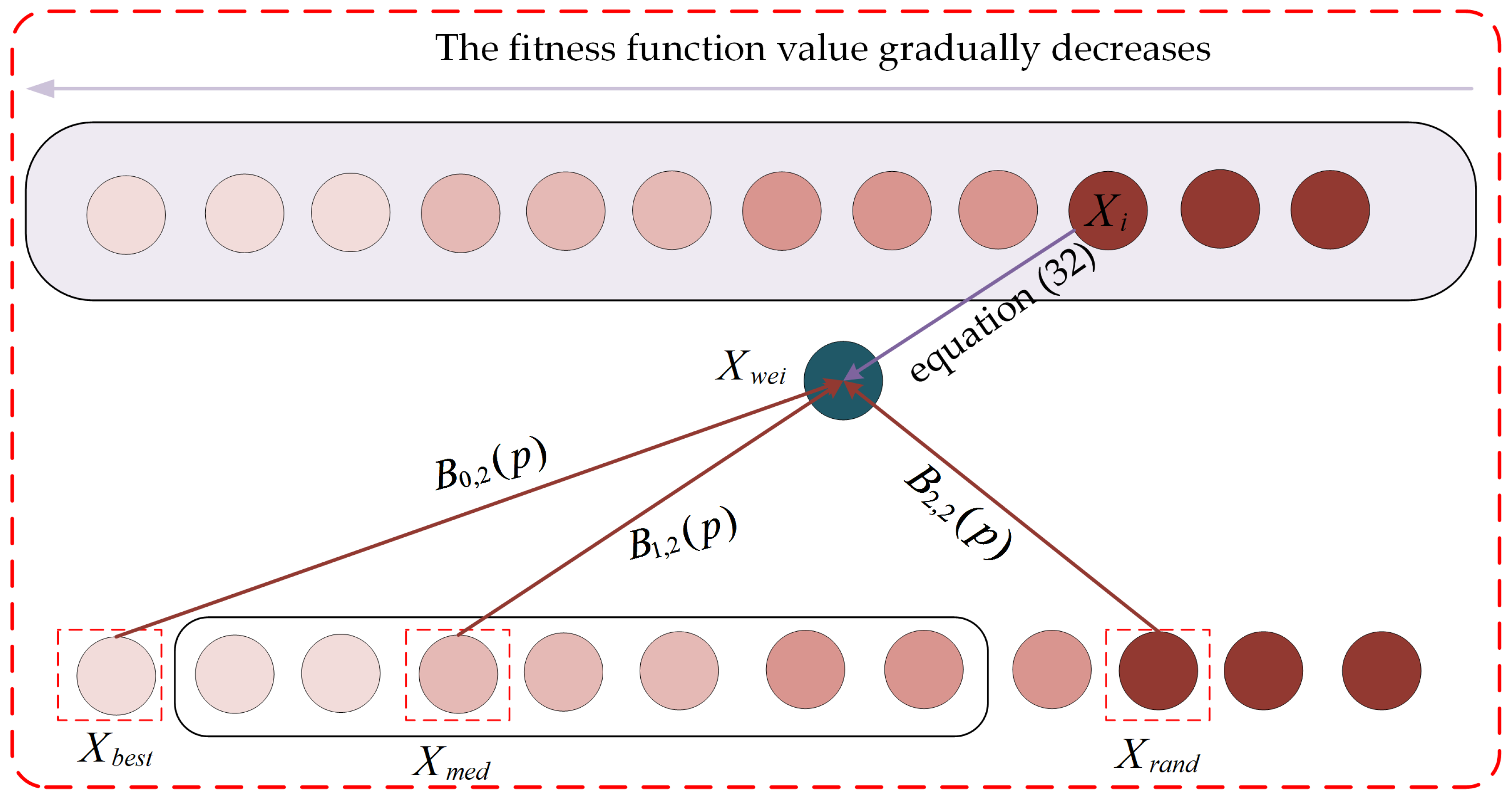
- A three-point guidance strategy based on Bernstein polynomials is proposed to enhance the local exploitation of the algorithm.
- Combining the above four learning strategies, the CLNBHEOA is proposed and applied to solve the multi-threshold image-segmentation problem to achieve better image-segmentation performance.
2. Related Works
2.1. Population Initialization Phase
2.2. Human Exploration Phase
2.3. Human Development Phase
2.3.1. Leaders Update Strategy
2.3.2. Explorers Update Strategy
2.3.3. Followers Update Strategy
2.3.4. Losers Update Strategy
2.4. Implementation of HEOA
| Algorithm 1: The pseudo-code of the HEOA |
|
Input: , , , , , Output: global best solution |
|
3. Proposed Model
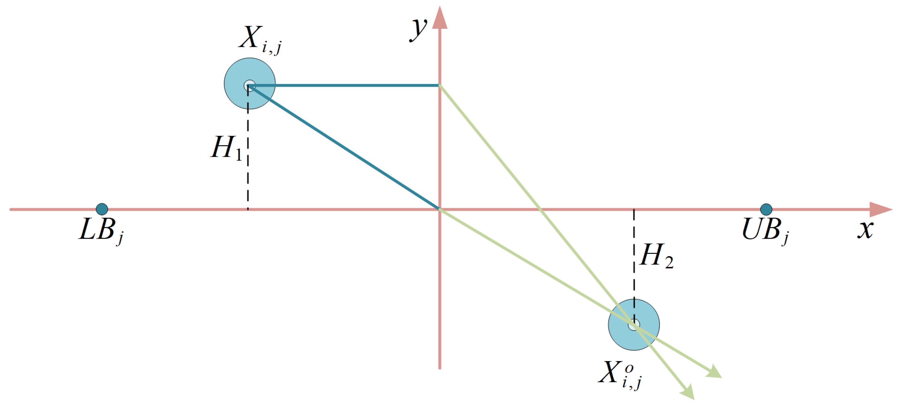
3.1. Chebyshev–Tent Chaotic Mapping Refraction Opposites-Based Learning Strategy
3.2. Adaptive Learning Strategy
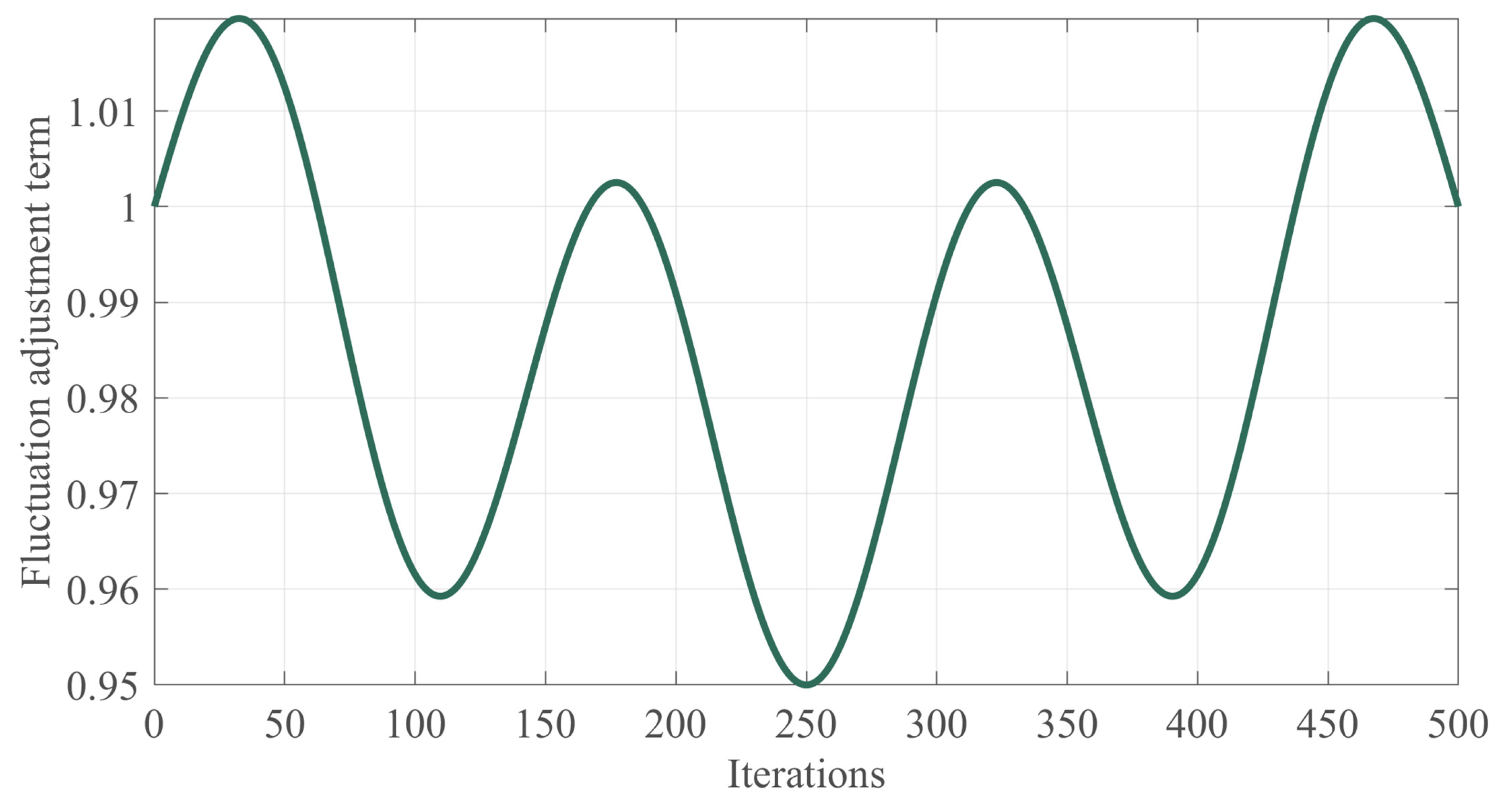
3.3. Nonlinear Control Factor
3.4. Three-Point Guidance Strategy Based on Bernstein Polynomials
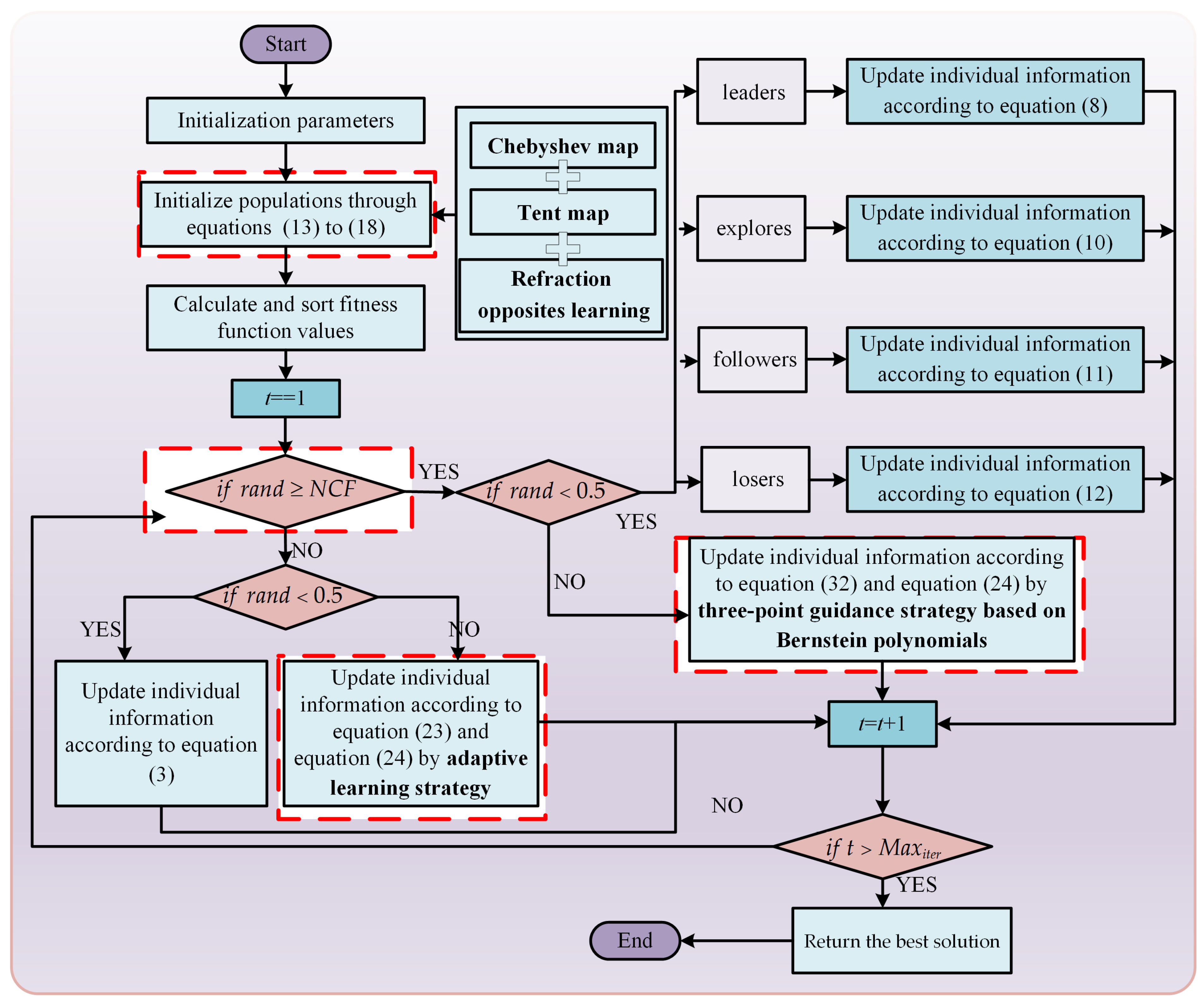
3.5. Implementation of the CLNBHEOA
| Algorithm 2: The pseudo-code associated with the CLNBHEOA |
|
Input: , , , , , Output: global best solution |
|
4. Experimental Procedure
5. Results
5.1. Experimental Results on CEC2017 Test Function
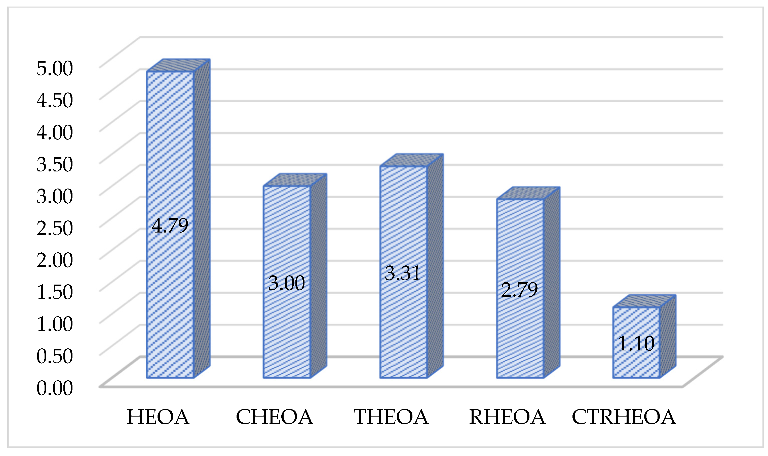
5.1.1. Validation of Initialization Strategy Effectiveness
5.1.2. Population Diversity Analysis
5.1.3. Exploration/Exploitation Balance Analysis
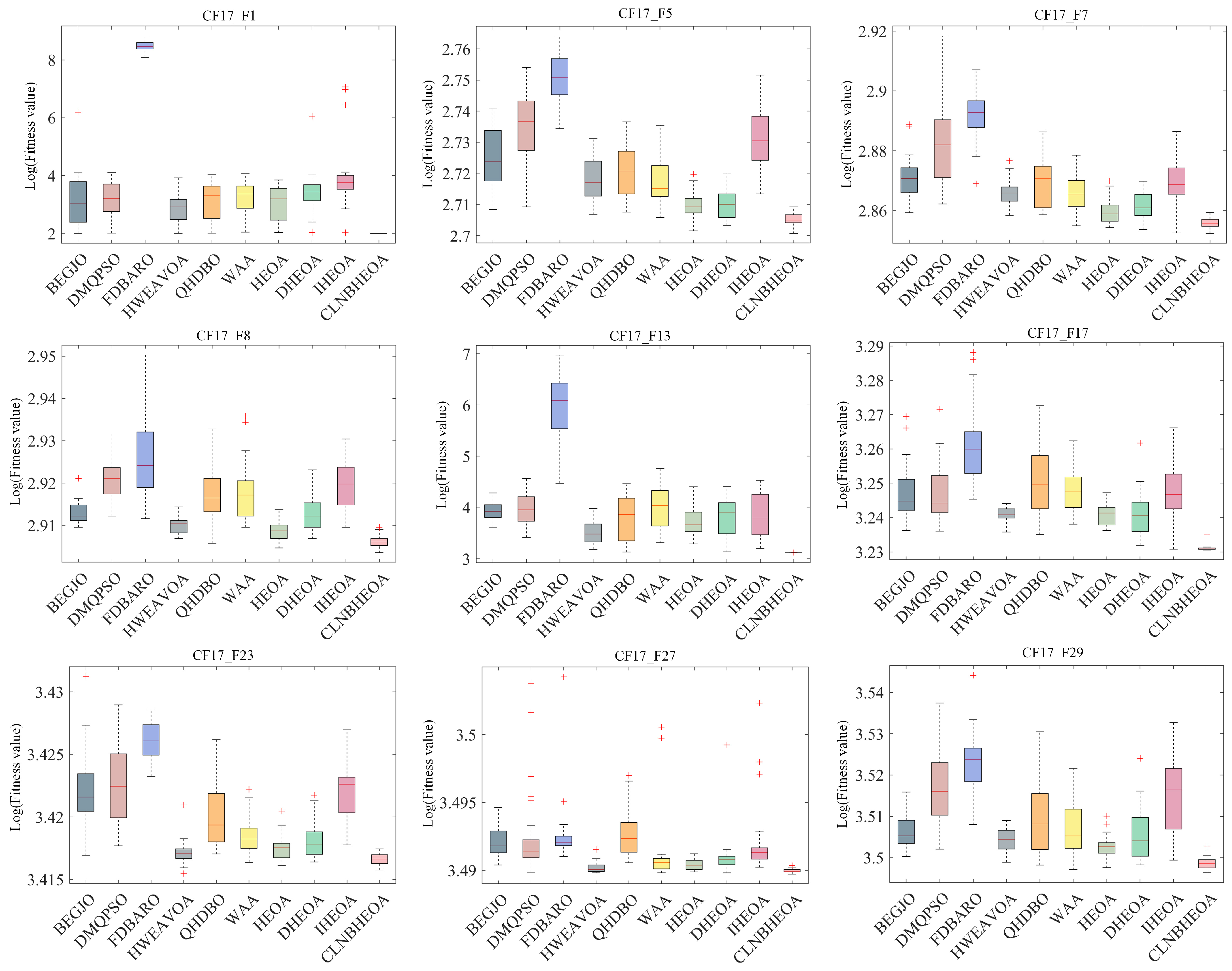
5.1.4. Fitness Function Value Analysis
5.1.5. Expansion Analysis of Fitness Function Values
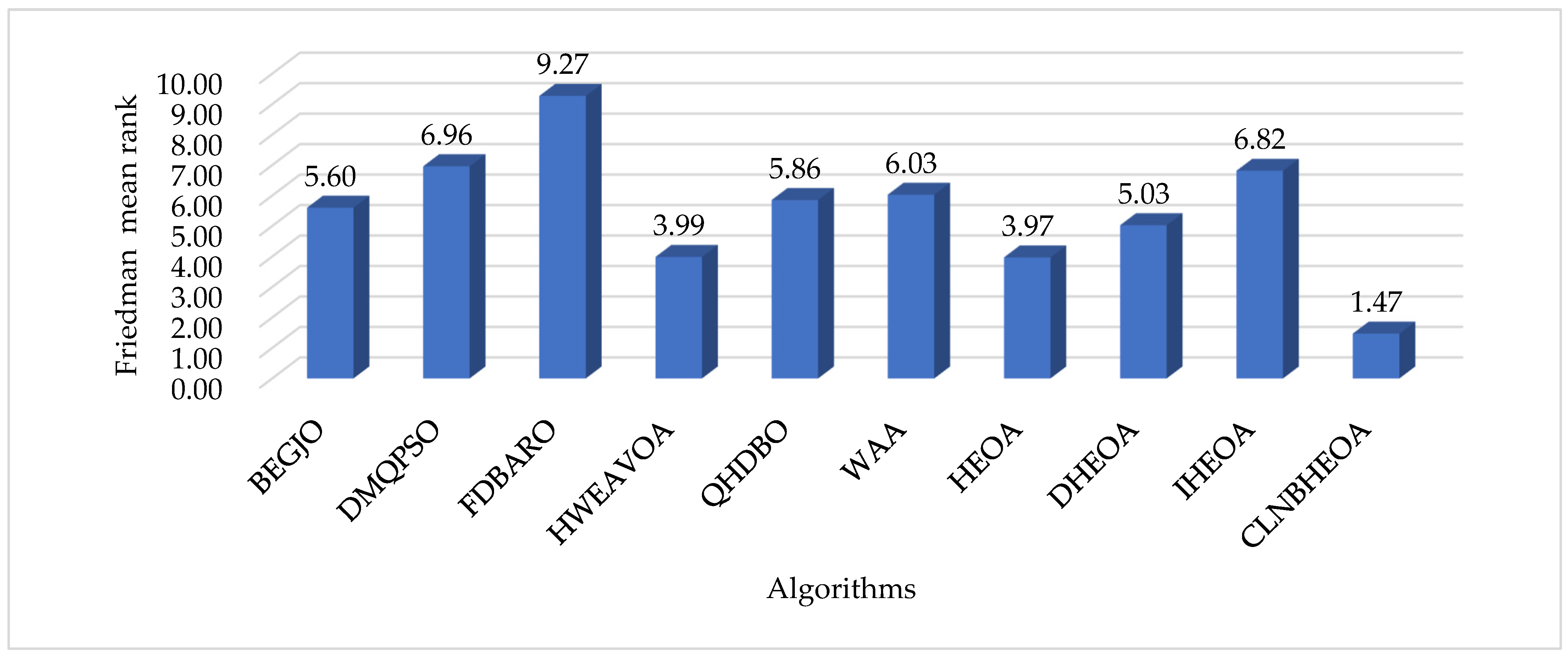
5.1.6. Nonparametric Rank-Sum Test Analysis
5.1.7. Convergence Analysis
5.2. Experimental Results on Multi-Threshold Image Segmentation
5.2.1. The Concept of Otsu Method
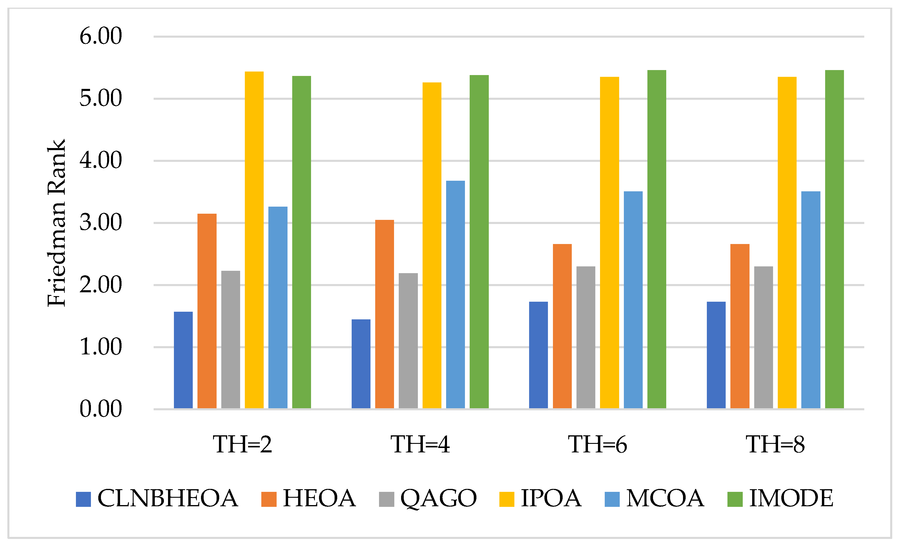
5.2.2. Experimental Results Analysis
6. Discussion
7. Conclusions
Author Contributions
Funding
Data Availability Statement
Acknowledgments
Conflicts of Interest
References
- Cao, W.; Martinis, S.; Plank, S. Automatic SAR-based flood detection using hierarchical tile-ranking thresholding and fuzzy logic. In Proceedings of the 2017 IEEE International Geoscience and Remote Sensing Symposium (IGARSS), Fort Worth, TX, USA, 23–28 July 2017; pp. 5697–5700. [Google Scholar]
- Santhos, K.A.; Kumar, A.; Bajaj, V.; Singh, G.K. McCulloch’s algorithm inspired cuckoo search optimizer based mammographic image segmentation. Multimed. Tools Appl. 2020, 79, 30453–30488. [Google Scholar] [CrossRef]
- Naito, T.; Tsukada, T.; Yamada, K.; Kozuka, K.; Yamamoto, S. Robust license-plate recognition method for passing vehicles under outside environment. IEEE Trans. Veh. Technol. 2000, 49, 2309–2319. [Google Scholar] [CrossRef]
- Huo, W.; Huang, Y.; Pei, J.; Liu, X.; Yang, J. Virtual SAR target image generation and similarity. In Proceedings of the 2016 IEEE International Geoscience and Remote Sensing Symposium (IGARSS), Beijing, China, 10–15 July 2016; pp. 914–917. [Google Scholar]
- Akay, B. A study on particle swarm optimization and artificial bee colony algorithms for multilevel thresholding. Appl. Soft Comput. 2013, 13, 3066–3091. [Google Scholar] [CrossRef]
- Wang, J.; Wang, N.; Wang, R. Research on medical image segmentation based on FCM algorithm. In Proceedings of the 2015 6th International Conference on Manufacturing Science and Engineering, Guangzhou, China, 28–29 November 2015; pp. 90–93. [Google Scholar]
- Heimowitz, A.; Keller, Y. Image segmentation via probabilistic graph matching. IEEE Trans. Image Process. 2017, 25, 4743–4752. [Google Scholar] [CrossRef]
- Wang, J.; Bei, J.; Song, H.; Zhang, H.; Zhang, P. A whale optimization algorithm with combined mutation and removing similarity for global optimization and multilevel thresholding image segmentation. Appl. Soft Comput. 2023, 137, 110130. [Google Scholar] [CrossRef]
- Otsu, N. A threshold selection method from gray-level histograms. Automatica 1975, 11, 23–27. [Google Scholar] [CrossRef]
- Dhanachandra, N.; Chanu, Y.J. An image segmentation approach based on fuzzy c-means and dynamic particle swarm optimization algorithm. Multimed. Tools Appl. 2020, 79, 18839–18858. [Google Scholar] [CrossRef]
- Hashim, F.A.; Hussien, A.G. Snake Optimizer: A novel meta-heuristic optimization algorithm. Knowl.-Based Syst. 2022, 242, 108320. [Google Scholar] [CrossRef]
- Holland, J.H. Genetic algorithms. Sci. Am. 1992, 267, 66–73. [Google Scholar] [CrossRef]
- Rocca, P.; Oliveri, G.; Massa, A. Differential evolution as applied to electromagnetics. IEEE Antennas Propag. Mag. 2011, 53, 38–49. [Google Scholar] [CrossRef]
- Beyer, H.G.; Schwefel, H.P. Evolution strategies—A comprehensive introduction. Nat. Comput. 2002, 1, 3–52. [Google Scholar] [CrossRef]
- Kennedy, J.; Eberhart, R. Particle swarm optimization. In Proceedings of the ICNN’95-International Conference on Neural Networks, Perth, Australia, 27 November–1 December 1995; pp. 1942–1948. [Google Scholar]
- Dorigo, M.; Birattari, M.; Stutzle, T. Ant colony optimization. IEEE Comput. Intell. Mag. 2007, 1, 28–39. [Google Scholar] [CrossRef]
- Mirjalili, S.; Mirjalili, S.M.; Lewis, A. Grey wolf optimizer. Adv. Eng. Softw. 2014, 69, 46–61. [Google Scholar] [CrossRef]
- Mirjalili, S.; Mirjalili, S.M.; Hatamlou, A. Multi-verse optimizer: A nature-inspired algorithm for global optimization. Neural Comput. Appl. 2016, 27, 495–513. [Google Scholar] [CrossRef]
- Tayarani-N, M.H.; Akbarzadeh-T, M.R. Magnetic-inspired optimization algorithms: Operators and structures. Swarm Evol. Comput. 2014, 19, 82–101. [Google Scholar] [CrossRef]
- Zhao, W.; Wang, L.; Zhang, Z. Atom search optimization and its application to solve a hydrogeologic parameter estimation problem. Knowl.-Based Syst. 2019, 163, 283–304. [Google Scholar] [CrossRef]
- Rao, R.V.; Savsani, V.J.; Vakharia, D.P. Teaching–learning-based optimization: A novel method for constrained mechanical design optimization problems. Comput.-Aided Des. 2011, 43, 303–315. [Google Scholar] [CrossRef]
- Shabani, A.; Asgarian, B.; Salido, M.; Gharebaghi, S.A. Search and rescue optimization algorithm: A new optimization method for solving constrained engineering optimization problems. Expert Syst. Appl. 2020, 161, 113698. [Google Scholar] [CrossRef]
- Das, B.; Mukherjee, V.; Das, D. Student psychology based optimization algorithm: A new population based optimization algorithm for solving optimization problems. Adv. Eng. Softw. 2020, 146, 102804. [Google Scholar] [CrossRef]
- Huang, C.; Li, X.; Wen, Y. AN OTSU image segmentation based on fruitfly optimization algorithm. Alex. Eng. J. 2021, 60, 183–188. [Google Scholar] [CrossRef]
- Ma, G.; Yue, X. An improved whale optimization algorithm based on multilevel threshold image segmentation using the Otsu method. Eng. Appl. Artif. Intell. 2022, 113, 104960. [Google Scholar] [CrossRef]
- Chen, L.; Gao, J.; Lopes, A.M.; Zhang, Z.; Chu, Z.; Wu, R. Adaptive fractional-order genetic-particle swarm optimization Otsu algorithm for image segmentation. Appl. Intell. 2023, 53, 26949–26966. [Google Scholar] [CrossRef]
- Qin, J.; Shen, X.; Mei, F.; Fang, Z. An Otsu multi-thresholds segmentation algorithm based on improved ACO. J. Supercomput. 2019, 75, 955–967. [Google Scholar] [CrossRef]
- Fan, Q.; Ma, Y.; Wang, P.; Bai, F. Otsu Image Segmentation Based on a Fractional Order Moth–Flame Optimization Algorithm. Fractal Fract. 2024, 8, 87. [Google Scholar] [CrossRef]
- Khairuzzaman, A.K.M.; Chaudhury, S. Multilevel thresholding using grey wolf optimizer for image segmentation. Expert Syst. Appl. 2017, 86, 64–76. [Google Scholar] [CrossRef]
- Wu, B.; Zhou, J.; Ji, X.; Yin, Y.; Shen, X. An ameliorated teaching–learning-based optimization algorithm based study of image segmentation for multilevel thresholding using Kapur’s entropy and Otsu’s between class variance. Inf. Sci. 2020, 533, 72–107. [Google Scholar] [CrossRef]
- Abd Elaziz, M.; Lu, S.; He, S. A multi-leader whale optimization algorithm for global optimization and image segmentation. Expert Syst. Appl. 2021, 175, 114841. [Google Scholar] [CrossRef]
- Lian, J.; Hui, G. Human evolutionary optimization algorithm. Expert Syst. Appl. 2024, 241, 122638. [Google Scholar] [CrossRef]
- Piotrowski, A.P.; Napiorkowski, J.J.; Piotrowska, A.E. Choice of benchmark optimization problems does matter. Swarm Evol. Comput. 2023, 83, 101378. [Google Scholar] [CrossRef]
- Li, X.D.; Wang, J.S.; Hao, W.K.; Zhang, M.; Wang, M. Chaotic arithmetic optimization algorithm. Appl. Intell. 2022, 52, 16718–16757. [Google Scholar] [CrossRef]
- Yang, Y.; Gao, Y.; Tan, S.; Zhao, S.; Wu, J.; Gao, S.; Wang, Y.G. An opposition learning and spiral modelling based arithmetic optimization algorithm for global continuous optimization problems. Eng. Appl. Artif. Intell. 2022, 113, 104981. [Google Scholar] [CrossRef]
- Zhang, Q.; Gao, H.; Zhan, Z.H.; Li, J.; Zhang, H. Growth Optimizer: A powerful metaheuristic algorithm for solving continuous and discrete global optimization problems. Knowl.-Based Syst. 2023, 261, 110206. [Google Scholar] [CrossRef]
- Elhoseny, M.; Abdel-salam, M.; El-Hasnony, I.M. An improved multi-strategy Golden Jackal algorithm for real world engineering problems. Knowl.-Based Syst. 2024, 295, 111725. [Google Scholar] [CrossRef]
- Zhang, X.; Lin, Q. Three-learning strategy particle swarm algorithm for global optimization problems. Inf. Sci. 2022, 593, 289–313. [Google Scholar] [CrossRef]
- Askr, H.; Abdel-Salam, M.; Hassanien, A.E. Copula entropy-based golden jackal optimization algorithm for high-dimensional feature selection problems. Expert Syst. Appl. 2024, 238, 121582. [Google Scholar] [CrossRef]
- Gong, C.; Zhou, N.; Xia, S.; Huang, S. Quantum particle swarm optimization algorithm based on diversity migration strategy. Future Gener. Comput. Syst. 2024, 157, 445–458. [Google Scholar] [CrossRef]
- Bakır, H. Dynamic fitness-distance balance-based artificial rabbits optimization algorithm to solve optimal power flow problem. Expert Syst. Appl. 2024, 240, 122460. [Google Scholar] [CrossRef]
- Wang, B.; Zhang, Z.; Siarry, P.; Liu, X.; Królczyk, G.; Hua, D.; Li, Z. A nonlinear African vulture optimization algorithm combining Henon chaotic mapping theory and reverse learning competition strategy. Expert Syst. Appl. 2024, 236, 121413. [Google Scholar] [CrossRef]
- Zhu, F.; Li, G.; Tang, H.; Li, Y.; Lv, X.; Wang, X. Dung beetle optimization algorithm based on quantum computing and multi-strategy fusion for solving engineering problems. Expert Syst. Appl. 2024, 236, 121219. [Google Scholar] [CrossRef]
- Cheng, J.; De Waele, W. Weighted average algorithm: A novel meta-heuristic optimization algorithm based on the weighted average position concept. Knowl.-Based Syst. 2024, 305, 112564. [Google Scholar] [CrossRef]
- Wang, Y.; Li, R.; Wang, Y.; Sun, J. Military UCAV 3D Path Planning Based on Multi-strategy Developed Human Evolutionary Optimization Algorithm. IEEE Internet Things J. early access. 2025. [Google Scholar] [CrossRef]
- Wang, X.; Zhou, S.; Wang, Z.; Xia, X.; Duan, Y. An Improved Human Evolution Optimization Algorithm for Unmanned Aerial Vehicle 3D Trajectory Planning. Biomimetics 2025, 10, 23. [Google Scholar] [CrossRef]
- Beşkirli, A.; Dağ, İ.; Kiran, M.S. A tree seed algorithm with multi-strategy for parameter estimation of solar photovoltaic models. Appl. Soft Comput. 2024, 167, 112220. [Google Scholar] [CrossRef]
- Beşkirli, A.; Dağ, İ. I-CPA: An improved carnivorous plant algorithm for solar photovoltaic parameter identification problem. Biomimetics 2023, 8, 569. [Google Scholar] [CrossRef]
- Huynh-Thu, Q.; Ghanbari, M. Scope of validity of PSNR in image/video quality assessment. Electron. Lett. 2008, 44, 800–801. [Google Scholar] [CrossRef]
- Wang, Z.; Bovik, A.C.; Sheikh, H.R.; Simoncelli, E.P. Image quality assessment: From error visibility to structural similarity. IEEE Trans. Image Process. 2004, 13, 600–612. [Google Scholar] [CrossRef] [PubMed]
- Zhang, L.; Zhang, L.; Mou, X.; Zhang, D. FSIM: A feature similarity index for image quality assessment. IEEE Trans. Image Process. 2011, 20, 2378–2386. [Google Scholar] [CrossRef]
- Gao, H.; Zhang, Q.; Bu, X.; Zhang, H. Quadruple parameter adaptation growth optimizer with integrated distribution, confrontation, and balance features for optimization. Expert Syst. Appl. 2024, 235, 121218. [Google Scholar] [CrossRef]
- SeyedGarmroudi, S.; Kayakutlu, G.; Kayalica, M.O.; Çolak, Ü. Improved Pelican optimization algorithm for solving load dispatch problems. Energy 2024, 289, 129811. [Google Scholar] [CrossRef]
- Jia, H.; Zhou, X.; Zhang, J.; Abualigah, L.; Yildiz, A.R.; Hussien, A.G. Modified crayfish optimization algorithm for solving multiple engineering application problems. Artif. Intell. Rev. 2024, 57, 127. [Google Scholar] [CrossRef]
- Sallam, K.M.; Elsayed, S.M.; Chakrabortty, R.K.; Ryan, M.J. Improved multi-operator differential evolution algorithm for solving unconstrained problems. In Proceedings of the 2020 IEEE Congress on Evolutionary Computation, Glasgow, UK, 19–24 July 2020; pp. 1–8. [Google Scholar]
- Beşkirli, A.; Dağ, İ. Parameter extraction for photovoltaic models with tree seed algorithm. Energy Rep. 2023, 9, 174–185. [Google Scholar] [CrossRef]
- Beşkirli, A.; Dağ, İ. An efficient tree seed inspired algorithm for parameter estimation of Photovoltaic models. Energy Rep. 2022, 8, 291–298. [Google Scholar] [CrossRef]


| Functions | Types | Name | Best |
|---|---|---|---|
| CF17_F1 | Unimodal | Shifted and Rotated Bent Cigar Function | 100 |
| CF17_F3 | Shifted and Rotated Zakharov Function | 300 | |
| CF17_F4 | Multimodal | Shifted and Rotated Rosenbrock’s Function | 400 |
| CF17_F5 | Shifted and Rotated Rastrigin’s Function | 500 | |
| CF17_F6 | Shifted and Rotated Expanded Scaffer’s F6 Function | 600 | |
| CF17_F7 | Shifted and Rotated Lunacek Bi-Rastrigin Function | 700 | |
| CF17_F8 | Shifted and Rotated Non-Continuous Rastrigin’s Function | 800 | |
| CF17_F9 | Shifted and Rotated Levy Function | 900 | |
| CF17_F10 | Shifted and Rotated Schwefel’s Function | 1000 | |
| CF17_F11 | Hybrid | Hybrid function 1 (N = 3) | 1100 |
| CF17_F12 | Hybrid function 1 (N = 3) | 1200 | |
| CF17_F13 | Hybrid function 3 (N = 3) | 1300 | |
| CF17_F14 | Hybrid function 4 (N = 4) | 1400 | |
| CF17_F15 | Hybrid function 5 (N = 4) | 1500 | |
| CF17_F16 | Hybrid function 6 (N = 4) | 1600 | |
| CF17_F17 | Hybrid function 6 (N = 5) | 1700 | |
| CF17_F18 | Hybrid function 6 (N = 5) | 1800 | |
| CF17_F19 | Hybrid function 6 (N = 5) | 1900 | |
| CF17_F20 | Hybrid function 6 (N = 6) | 2000 | |
| CF17_F21 | Composition | Composition function 1 (N = 3) | 2100 |
| CF17_F22 | Composition function 2 (N = 3) | 2200 | |
| CF17_F23 | Composition function 3 (N = 4) | 2300 | |
| CF17_F24 | Composition function 4 (N = 4) | 2400 | |
| CF17_F25 | Composition function 5 (N = 5) | 2500 | |
| CF17_F26 | Composition function 6 (N = 5) | 2600 | |
| CF17_F27 | Composition function 7 (N = 6) | 2700 | |
| CF17_F28 | Composition function 8 (N = 6) | 2800 | |
| CF17_F29 | Composition function 9 (N = 3) | 2900 | |
| CF17_F30 | Composition function 10 (N = 3) | 3000 |
| Algorithms | Time | Parameters |
|---|---|---|
| Binary Enhanced Golden Jackal Optimization (BEGJO) [39] | 2024 | |
| DMQPSO [40] | 2024 | |
| Fitness-Distance Balance-Based Artificial Rabbits Optimization (FDBARO) [41] | 2024 | No Parameters |
| HWEAVOA [42] | 2024 | |
| QHDBO [43] | 2024 | |
| Weighted Average Algorithm (WAA) [44] | 2024 | |
| Human Evolutionary Optimization Algorithm (HEOA) | 2024 | |
| Developed Human Evolutionary Optimization Algorithm (DHEOA) [45] | 2025 | |
| Improved Human Evolution Optimization Algorithm (IHEOA) [46] | 2025 | |
| MS-TSA [47] | 2024 | |
| I-CPA [48] | 2023 | No Parameters |
| Functions | Metrics | BEGJO | DMQPSO | FDBARO | HWEAVOA | QHDBO | WAA | HEOA | DHEOA | IHEOA | CLNBHEOA |
|---|---|---|---|---|---|---|---|---|---|---|---|
| CF17_F1 | Mean | 5.470 × 10+04 | 3.042 × 10+03 | 3.238 × 10+08 | 1.554 × 10+03 | 2.964 × 10+03 | 3.112 × 10+03 | 2.226 × 10+03 | 4.028 × 10+04 | 7.981 × 10+05 | 1.000 × 10+02 |
| Std | 2.823 × 10+05 | 3.299 × 10+03 | 1.432 × 10+08 | 1.981 × 10+03 | 3.317 × 10+03 | 3.214 × 10+03 | 2.134 × 10+03 | 2.036 × 10+05 | 2.707 × 10+06 | 4.594 × 10⁻¹⁴ | |
| CF17_F3 | Mean | 3.003 × 10+02 | 3.037 × 10+02 | 2.684 × 10+03 | 3.062 × 10+02 | 3.027 × 10+02 | 3.000 × 10+02 | 3.000 × 10+02 | 3.000 × 10+02 | 3.116 × 10+02 | 3.000 × 10+02 |
| Std | 5.481 × 10−01 | 1.317 × 10+01 | 2.348 × 10+03 | 1.516 × 10+01 | 6.232 × 10+00 | 1.598 × 10−09 | 4.088 × 10⁻¹⁰ | 4.104 × 10−02 | 4.514 × 10+01 | 4.352 × 10⁻¹⁴ | |
| CF17_F4 | Mean | 4.126 × 10+02 | 4.067 × 10+02 | 4.336 × 10+02 | 4.024 × 10+02 | 4.072 × 10+02 | 4.078 × 10+02 | 4.034 × 10+02 | 4.095 × 10+02 | 4.309 × 10+02 | 4.000 × 10+02 |
| Std | 1.754 × 10+01 | 1.198 × 10+01 | 2.297 × 10+01 | 1.268 × 10+00 | 1.278 × 10+01 | 1.441 × 10+01 | 1.423 × 10+00 | 1.599 × 10+01 | 4.480 × 10+01 | 2.396 × 10−08 | |
| CF17_F5 | Mean | 5.311 × 10+02 | 5.434 × 10+02 | 5.635 × 10+02 | 5.221 × 10+02 | 5.250 × 10+02 | 5.218 × 10+02 | 5.125 × 10+02 | 5.134 × 10+02 | 5.386 × 10+02 | 5.072 × 10+02 |
| Std | 1.147 × 10+01 | 1.355 × 10+01 | 9.144 × 10+00 | 8.424 × 10+00 | 9.635 × 10+00 | 8.405 × 10+00 | 5.047 × 10+00 | 5.540 × 10+00 | 1.194 × 10+01 | 2.286 × 10+00 | |
| CF17_F6 | Mean | 6.012 × 10+02 | 6.174 × 10+02 | 6.126 × 10+02 | 6.003 × 10+02 | 6.005 × 10+02 | 6.157 × 10+02 | 6.006 × 10+02 | 6.005 × 10+02 | 6.107 × 10+02 | 6.000 × 10+02 |
| Std | 2.533 × 10+00 | 8.682 × 10+00 | 4.898 × 10+00 | 8.496 × 10−01 | 7.983 × 10−01 | 1.253 × 10+01 | 1.459 × 10+00 | 9.855 × 10−01 | 7.438 × 10+00 | 1.198 × 10−05 | |
| CF17_F7 | Mean | 7.430 × 10+02 | 7.625 × 10+02 | 7.796 × 10+02 | 7.334 × 10+02 | 7.404 × 10+02 | 7.348 × 10+02 | 7.240 × 10+02 | 7.272 × 10+02 | 7.402 × 10+02 | 7.176 × 10+02 |
| Std | 1.193 × 10+01 | 2.254 × 10+01 | 1.380 × 10+01 | 7.288 × 10+00 | 1.286 × 10+01 | 9.414 × 10+00 | 6.465 × 10+00 | 7.060 × 10+00 | 1.132 × 10+01 | 2.921 × 10+00 | |
| CF17_F8 | Mean | 8.184 × 10+02 | 8.336 × 10+02 | 8.434 × 10+02 | 8.130 × 10+02 | 8.269 × 10+02 | 8.281 × 10+02 | 8.106 × 10+02 | 8.182 × 10+02 | 8.310 × 10+02 | 8.057 × 10+02 |
| Std | 4.802 × 10+00 | 8.803 × 10+00 | 1.669 × 10+01 | 3.648 × 10+00 | 1.207 × 10+01 | 1.305 × 10+01 | 4.177 × 10+00 | 7.527 × 10+00 | 1.094 × 10+01 | 2.292 × 10+00 | |
| CF17_F9 | Mean | 9.088 × 10+02 | 1.147 × 10+03 | 9.435 × 10+02 | 9.096 × 10+02 | 9.195 × 10+02 | 9.551 × 10+02 | 9.020 × 10+02 | 9.022 × 10+02 | 9.743 × 10+02 | 9.000 × 10+02 |
| Std | 2.286 × 10+01 | 1.982 × 10+02 | 3.116 × 10+01 | 3.055 × 10+01 | 4.565 × 10+01 | 1.045 × 10+02 | 3.980 × 10+00 | 4.838 × 10+00 | 1.139 × 10+02 | 0.000 × 10+00 | |
| CF17_F10 | Mean | 1.554 × 10+03 | 1.870 × 10+03 | 2.581 × 10+03 | 1.639 × 10+03 | 1.852 × 10+03 | 1.898 × 10+03 | 1.986 × 10+03 | 1.734 × 10+03 | 1.995 × 10+03 | 1.299 × 10+03 |
| Std | 2.869 × 10+02 | 3.439 × 10+02 | 4.125 × 10+02 | 1.752 × 10+02 | 2.865 × 10+02 | 2.944 × 10+02 | 2.801 × 10+02 | 3.176 × 10+02 | 3.067 × 10+02 | 1.419 × 10+02 | |
| CF17_F11 | Mean | 1.124 × 10+03 | 1.159 × 10+03 | 1.213 × 10+03 | 1.109 × 10+03 | 1.114 × 10+03 | 1.162 × 10+03 | 1.118 × 10+03 | 1.128 × 10+03 | 1.227 × 10+03 | 1.101 × 10+03 |
| Std | 1.006 × 10+01 | 5.745 × 10+01 | 9.193 × 10+01 | 5.848 × 10+00 | 1.267 × 10+01 | 4.330 × 10+01 | 1.898 × 10+01 | 2.979 × 10+01 | 1.120 × 10+02 | 1.298 × 10+00 | |
| CF17_F12 | Mean | 7.460 × 10+03 | 6.561 × 10+05 | 2.192 × 10+07 | 9.042 × 10+03 | 1.829 × 10+06 | 2.340 × 10+06 | 1.667 × 10+04 | 2.972 × 10+04 | 1.908 × 10+06 | 1.321 × 10+03 |
| Std | 2.941 × 10+03 | 8.157 × 10+05 | 1.941 × 10+07 | 4.121 × 10+03 | 3.708 × 10+06 | 1.941 × 10+06 | 1.596 × 10+04 | 8.597 × 10+04 | 3.230 × 10+06 | 9.833 × 10+01 | |
| CF17_F13 | Mean | 9.174 × 10+03 | 1.243 × 10+04 | 1.792 × 10+06 | 3.738 × 10+03 | 9.062 × 10+03 | 1.461 × 10+04 | 7.015 × 10+03 | 8.635 × 10+03 | 1.174 × 10+04 | 1.307 × 10+03 |
| Std | 3.531 × 10+03 | 9.746 × 10+03 | 2.050 × 10+06 | 2.101 × 10+03 | 7.772 × 10+03 | 1.274 × 10+04 | 5.612 × 10+03 | 6.017 × 10+03 | 1.151 × 10+04 | 3.204 × 10+00 | |
| CF17_F14 | Mean | 1.488 × 10+03 | 2.170 × 10+03 | 2.813 × 10+05 | 1.504 × 10+03 | 1.527 × 10+03 | 1.645 × 10+03 | 1.478 × 10+03 | 1.466 × 10+03 | 1.719 × 10+03 | 1.402 × 10+03 |
| Std | 3.098 × 10+01 | 9.216 × 10+02 | 5.167 × 10+05 | 2.896 × 10+01 | 6.726 × 10+01 | 3.296 × 10+02 | 2.411 × 10+01 | 6.426 × 10+01 | 4.939 × 10+02 | 1.071 × 10+00 | |
| CF17_F15 | Mean | 2.040 × 10+03 | 4.224 × 10+03 | 3.891 × 10+04 | 1.819 × 10+03 | 2.142 × 10+03 | 3.961 × 10+03 | 1.704 × 10+03 | 2.519 × 10+03 | 2.417 × 10+03 | 1.501 × 10+03 |
| Std | 9.606 × 10+02 | 2.692 × 10+03 | 6.415 × 10+04 | 2.698 × 10+02 | 8.484 × 10+02 | 2.675 × 10+03 | 9.180 × 10+01 | 1.076 × 10+03 | 9.134 × 10+02 | 1.072 × 10+00 | |
| CF17_F16 | Mean | 1.748 × 10+03 | 1.763 × 10+03 | 1.870 × 10+03 | 1.679 × 10+03 | 1.742 × 10+03 | 1.755 × 10+03 | 1.623 × 10+03 | 1.709 × 10+03 | 1.754 × 10+03 | 1.613 × 10+03 |
| Std | 1.495 × 10+02 | 1.221 × 10+02 | 1.415 × 10+02 | 6.130 × 10+01 | 1.053 × 10+02 | 1.119 × 10+02 | 4.034 × 10+01 | 8.813 × 10+01 | 1.212 × 10+02 | 3.112 × 10+01 | |
| CF17_F17 | Mean | 1.768 × 10+03 | 1.767 × 10+03 | 1.827 × 10+03 | 1.742 × 10+03 | 1.782 × 10+03 | 1.771 × 10+03 | 1.741 × 10+03 | 1.742 × 10+03 | 1.769 × 10+03 | 1.703 × 10+03 |
| Std | 3.236 × 10+01 | 3.434 × 10+01 | 5.324 × 10+01 | 7.993 × 10+00 | 3.992 × 10+01 | 2.714 × 10+01 | 1.266 × 10+01 | 2.539 × 10+01 | 3.142 × 10+01 | 4.960 × 10+00 | |
| CF17_F18 | Mean | 5.919 × 10+03 | 1.516 × 10+04 | 8.325 × 10+06 | 2.971 × 10+03 | 1.052 × 10+04 | 2.042 × 10+04 | 8.224 × 10+03 | 1.306 × 10+04 | 1.878 × 10+04 | 1.805 × 10+03 |
| Std | 5.329 × 10+03 | 1.214 × 10+04 | 1.013 × 10+07 | 1.177 × 10+03 | 8.408 × 10+03 | 1.230 × 10+04 | 5.657 × 10+03 | 1.063 × 10+04 | 1.606 × 10+04 | 7.734 × 10+00 | |
| CF17_F19 | Mean | 1.956 × 10+03 | 9.568 × 10+03 | 8.819 × 10+05 | 2.216 × 10+03 | 3.366 × 10+03 | 4.883 × 10+03 | 2.028 × 10+03 | 8.424 × 10+03 | 5.161 × 10+03 | 1.900 × 10+03 |
| Std | 4.675 × 10+01 | 9.040 × 10+03 | 1.899 × 10+06 | 5.089 × 10+02 | 2.112 × 10+03 | 3.225 × 10+03 | 1.052 × 10+02 | 6.840 × 10+03 | 6.896 × 10+03 | 3.722 × 10−01 | |
| CF17_F20 | Mean | 2.046 × 10+03 | 2.133 × 10+03 | 2.185 × 10+03 | 2.032 × 10+03 | 2.061 × 10+03 | 2.114 × 10+03 | 2.022 × 10+03 | 2.092 × 10+03 | 2.097 × 10+03 | 2.001 × 10+03 |
| Std | 1.831 × 10+01 | 7.504 × 10+01 | 6.224 × 10+01 | 1.590 × 10+01 | 4.496 × 10+01 | 6.861 × 10+01 | 1.060 × 10+01 | 5.782 × 10+01 | 5.656 × 10+01 | 1.151 × 10+00 | |
| CF17_F21 | Mean | 2.314 × 10+03 | 2.271 × 10+03 | 2.350 × 10+03 | 2.256 × 10+03 | 2.322 × 10+03 | 2.283 × 10+03 | 2.277 × 10+03 | 2.286 × 10+03 | 2.232 × 10+03 | 2.248 × 10+03 |
| Std | 4.398 × 10+01 | 6.876 × 10+01 | 2.830 × 10+01 | 5.517 × 10+01 | 2.455 × 10+01 | 5.881 × 10+01 | 4.913 × 10+01 | 4.787 × 10+01 | 5.263 × 10+01 | 5.603 × 10+01 | |
| CF17_F22 | Mean | 2.272 × 10+03 | 2.308 × 10+03 | 2.338 × 10+03 | 2.300 × 10+03 | 2.303 × 10+03 | 2.297 × 10+03 | 2.297 × 10+03 | 2.300 × 10+03 | 2.310 × 10+03 | 2.294 × 10+03 |
| Std | 4.078 × 10+01 | 4.584 × 10+00 | 1.613 × 10+01 | 1.415 × 10+00 | 2.244 × 10+00 | 2.359 × 10+01 | 1.946 × 10+01 | 1.171 × 10+01 | 7.111 × 10+00 | 2.406 × 10+01 | |
| CF17_F23 | Mean | 2.644 × 10+03 | 2.645 × 10+03 | 2.668 × 10+03 | 2.613 × 10+03 | 2.630 × 10+03 | 2.621 × 10+03 | 2.615 × 10+03 | 2.619 × 10+03 | 2.642 × 10+03 | 2.610 × 10+03 |
| Std | 1.779 × 10+01 | 1.876 × 10+01 | 8.838 × 10+00 | 5.935 × 10+00 | 1.528 × 10+01 | 8.681 × 10+00 | 5.536 × 10+00 | 8.574 × 10+00 | 1.349 × 10+01 | 2.528 × 10+00 | |
| CF17_F24 | Mean | 2.737 × 10+03 | 2.765 × 10+03 | 2.800 × 10+03 | 2.718 × 10+03 | 2.758 × 10+03 | 2.741 × 10+03 | 2.704 × 10+03 | 2.744 × 10+03 | 2.671 × 10+03 | 2.644 × 10+03 |
| Std | 1.101 × 10+02 | 7.559 × 10+01 | 1.272 × 10+01 | 6.500 × 10+01 | 1.164 × 10+01 | 4.663 × 10+01 | 8.007 × 10+01 | 8.141 × 10+00 | 1.157 × 10+02 | 1.196 × 10+02 | |
| CF17_F25 | Mean | 2.922 × 10+03 | 2.937 × 10+03 | 2.950 × 10+03 | 2.927 × 10+03 | 2.923 × 10+03 | 2.917 × 10+03 | 2.924 × 10+03 | 2.935 × 10+03 | 2.941 × 10+03 | 2.912 × 10+03 |
| Std | 2.271 × 10+01 | 2.824 × 10+01 | 2.121 × 10+01 | 2.090 × 10+01 | 2.375 × 10+01 | 6.672 × 10+01 | 2.334 × 10+01 | 2.052 × 10+01 | 2.637 × 10+01 | 2.112 × 10+01 | |
| CF17_F26 | Mean | 2.947 × 10+03 | 3.118 × 10+03 | 3.266 × 10+03 | 2.907 × 10+03 | 3.215 × 10+03 | 2.965 × 10+03 | 2.941 × 10+03 | 3.010 × 10+03 | 3.023 × 10+03 | 2.905 × 10+03 |
| Std | 2.533 × 10+02 | 3.427 × 10+02 | 4.882 × 10+02 | 6.786 × 10+01 | 3.558 × 10+02 | 2.843 × 10+02 | 8.060 × 10+01 | 2.247 × 10+02 | 1.445 × 10+02 | 1.798 × 10+01 | |
| CF17_F27 | Mean | 3.105 × 10+03 | 3.108 × 10+03 | 3.109 × 10+03 | 3.092 × 10+03 | 3.110 × 10+03 | 3.098 × 10+03 | 3.093 × 10+03 | 3.097 × 10+03 | 3.105 × 10+03 | 3.090 × 10+03 |
| Std | 8.564 × 10+00 | 2.311 × 10+01 | 1.684 × 10+01 | 2.763 × 10+00 | 1.199 × 10+01 | 1.791 × 10+01 | 3.020 × 10+00 | 1.173 × 10+01 | 1.850 × 10+01 | 9.345 × 10−01 | |
| CF17_F28 | Mean | 3.459 × 10+03 | 3.308 × 10+03 | 3.381 × 10+03 | 3.209 × 10+03 | 3.328 × 10+03 | 3.273 × 10+03 | 3.267 × 10+03 | 3.337 × 10+03 | 3.300 × 10+03 | 3.230 × 10+03 |
| Std | 1.364 × 10+02 | 1.528 × 10+02 | 1.103 × 10+02 | 1.320 × 10+02 | 1.181 × 10+02 | 1.474 × 10+02 | 1.362 × 10+02 | 9.853 × 10+01 | 1.018 × 10+02 | 1.509 × 10+02 | |
| CF17_F29 | Mean | 3.206 × 10+03 | 3.286 × 10+03 | 3.336 × 10+03 | 3.193 × 10+03 | 3.232 × 10+03 | 3.211 × 10+03 | 3.181 × 10+03 | 3.202 × 10+03 | 3.276 × 10+03 | 3.152 × 10+03 |
| Std | 2.861 × 10+01 | 7.563 × 10+01 | 5.761 × 10+01 | 2.078 × 10+01 | 6.186 × 10+01 | 4.800 × 10+01 | 1.967 × 10+01 | 4.596 × 10+01 | 6.796 × 10+01 | 1.063 × 10+01 | |
| CF17_F30 | Mean | 9.854 × 10+04 | 3.599 × 10+05 | 2.222 × 10+06 | 9.285 × 10+04 | 3.151 × 10+05 | 4.437 × 10+05 | 3.566 × 10+05 | 2.669 × 10+05 | 6.622 × 10+05 | 3.514 × 10+03 |
| Std | 2.735 × 10+05 | 4.322 × 10+05 | 3.032 × 10+06 | 2.059 × 10+05 | 4.422 × 10+05 | 6.321 × 10+05 | 4.681 × 10+05 | 4.822 × 10+05 | 7.298 × 10+05 | 8.863 × 10+01 | |
| Mean Rank | 5.14 | 7.69 | 9.72 | 3.24 | 6.07 | 6.34 | 3.21 | 5.03 | 7.31 | 1.10 | |
| Final Rank | 5 | 9 | 10 | 3 | 6 | 7 | 2 | 4 | 8 | 1 | |
| Functions | Metrics | MS-TSA | I-CPA | FDBARO | HWEAVOA | QHDBO | WAA | HEOA | DHEOA | IHEOA | CLNBHEOA |
|---|---|---|---|---|---|---|---|---|---|---|---|
| CF17_F1 | Mean | 4.370 × 10+03 | 6.580 × 10+09 | 3.853 × 10+08 | 1.792 × 10+03 | 2.230 × 10+03 | 1.711 × 10+03 | 1.350 × 10+03 | 2.277 × 10+03 | 6.436 × 10+03 | 1.000 × 10+02 |
| Std | 5.600 × 10+03 | 4.510 × 10+09 | 3.200 × 10+08 | 1.923 × 10+03 | 2.534 × 10+03 | 2.142 × 10+03 | 1.606 × 10+03 | 2.541 × 10+03 | 4.242 × 10+03 | 0.000 × 10+00 | |
| CF17_F3 | Mean | 8.120 × 10+03 | 5.220 × 10+04 | 2.396 × 10+03 | 3.000 × 10+02 | 3.000 × 10+02 | 3.000 × 10+02 | 3.000 × 10+02 | 3.000 × 10+02 | 3.000 × 10+02 | 3.000 × 10+02 |
| Std | 3.150 × 10+03 | 8.930 × 10+03 | 2.063 × 10+03 | 1.007 × 10⁻¹³ | 6.064 × 10⁻¹⁴ | 3.309 × 10⁻¹⁰ | 8.039 × 10⁻¹⁴ | 1.185 × 10⁻¹³ | 2.728 × 10⁻¹³ | 0.000 × 10+00 | |
| CF17_F4 | Mean | 4.530 × 10+02 | 1.840 × 10+03 | 4.272 × 10+02 | 4.001 × 10+02 | 4.028 × 10+02 | 4.001 × 10+02 | 4.000 × 10+02 | 4.003 × 10+02 | 4.104 × 10+02 | 4.000 × 10+02 |
| Std | 3.390 × 10+01 | 1.090 × 10+03 | 1.720 × 10+01 | 2.526 × 10−02 | 1.884 × 10+00 | 2.380 × 10−01 | 2.060 × 10−02 | 1.440 × 10−01 | 1.528 × 10+01 | 0.000 × 10+00 | |
| CF17_F5 | Mean | 6.240 × 10+02 | 7.280 × 10+02 | 5.538 × 10+02 | 5.147 × 10+02 | 5.224 × 10+02 | 5.159 × 10+02 | 5.100 × 10+02 | 5.136 × 10+02 | 5.267 × 10+02 | 5.066 × 10+02 |
| Std | 6.570 × 10+01 | 4.900 × 10+01 | 1.029 × 10+01 | 6.363 × 10+00 | 8.643 × 10+00 | 6.316 × 10+00 | 3.606 × 10+00 | 6.456 × 10+00 | 1.244 × 10+01 | 2.283 × 10+00 | |
| CF17_F6 | Mean | 6.000 × 10+02 | 6.420 × 10+02 | 6.115 × 10+02 | 6.001 × 10+02 | 6.003 × 10+02 | 6.018 × 10+02 | 6.003 × 10+02 | 6.002 × 10+02 | 6.073 × 10+02 | 6.000 × 10+02 |
| Std | 2.350 × 10−01 | 7.320 × 10+00 | 2.965 × 10+00 | 2.009 × 10−01 | 4.866 × 10−01 | 2.426 × 10+00 | 7.679 × 10−01 | 5.185 × 10−01 | 6.315 × 10+00 | 2.111 × 10⁻¹⁴ | |
| CF17_F7 | Mean | 8.960 × 10+02 | 1.100 × 10+03 | 7.770 × 10+02 | 7.300 × 10+02 | 7.256 × 10+02 | 7.279 × 10+02 | 7.190 × 10+02 | 7.259 × 10+02 | 7.439 × 10+02 | 7.182 × 10+02 |
| Std | 5.010 × 10+01 | 8.140 × 10+01 | 1.099 × 10+01 | 7.209 × 10+00 | 9.149 × 10+00 | 8.671 × 10+00 | 4.072 × 10+00 | 6.837 × 10+00 | 1.197 × 10+01 | 3.557 × 10+00 | |
| CF17_F8 | Mean | 9.280 × 10+02 | 9.930 × 10+02 | 8.366 × 10+02 | 8.090 × 10+02 | 8.213 × 10+02 | 8.159 × 10+02 | 8.093 × 10+02 | 8.131 × 10+02 | 8.284 × 10+02 | 8.053 × 10+02 |
| Std | 6.630 × 10+01 | 3.510 × 10+01 | 9.495 × 10+00 | 2.629 × 10+00 | 6.345 × 10+00 | 6.868 × 10+00 | 3.108 × 10+00 | 4.638 × 10+00 | 8.632 × 10+00 | 1.597 × 10+00 | |
| CF17_F9 | Mean | 9.010 × 10+02 | 5.470 × 10+03 | 9.486 × 10+02 | 9.002 × 10+02 | 9.020 × 10+02 | 9.011 × 10+02 | 9.015 × 10+02 | 9.017 × 10+02 | 9.436 × 10+02 | 9.000 × 10+02 |
| Std | 1.140 × 10+00 | 1.600 × 10+03 | 4.633 × 10+01 | 4.684 × 10−01 | 5.830 × 10+00 | 2.234 × 10+00 | 2.265 × 10+00 | 8.098 × 10+00 | 6.363 × 10+01 | 0.000 × 10+00 | |
| CF17_F10 | Mean | 7.100 × 10+03 | 6.000 × 10+03 | 2.377 × 10+03 | 1.435 × 10+03 | 1.745 × 10+03 | 1.645 × 10+03 | 1.304 × 10+03 | 1.591 × 10+03 | 1.790 × 10+03 | 1.279 × 10+03 |
| Std | 1.530 × 10+03 | 6.680 × 10+02 | 4.389 × 10+02 | 1.395 × 10+02 | 2.904 × 10+02 | 2.182 × 10+02 | 1.986 × 10+02 | 2.558 × 10+02 | 2.855 × 10+02 | 1.794 × 10+02 | |
| CF17_F11 | Mean | 1.170 × 10+03 | 3.490 × 10+03 | 1.181 × 10+03 | 1.104 × 10+03 | 1.112 × 10+03 | 1.133 × 10+03 | 1.111 × 10+03 | 1.116 × 10+03 | 1.173 × 10+03 | 1.101 × 10+03 |
| Std | 4.890 × 10+01 | 1.810 × 10+03 | 5.112 × 10+01 | 3.404 × 10+00 | 8.111 × 10+00 | 2.325 × 10+01 | 1.009 × 10+01 | 8.447 × 10+00 | 6.107 × 10+01 | 1.207 × 10+00 | |
| CF17_F12 | Mean | 2.060 × 10+05 | 6.370 × 10+08 | 2.275 × 10+07 | 6.805 × 10+03 | 3.021 × 10+05 | 1.957 × 10+04 | 1.079 × 10+04 | 1.188 × 10+04 | 5.464 × 10+05 | 1.294 × 10+03 |
| Std | 1.140 × 10+05 | 7.140 × 10+08 | 3.035 × 10+07 | 2.654 × 10+03 | 6.095 × 10+05 | 1.824 × 10+04 | 1.040 × 10+04 | 1.091 × 10+04 | 1.796 × 10+06 | 9.653 × 10+01 | |
| CF17_F13 | Mean | 1.480 × 10+04 | 6.370 × 10+08 | 1.155 × 10+06 | 2.416 × 10+03 | 2.522 × 10+03 | 1.052 × 10+04 | 1.949 × 10+03 | 7.999 × 10+03 | 8.345 × 10+03 | 1.307 × 10+03 |
| Std | 1.480 × 10+04 | 1.320 × 10+09 | 1.439 × 10+06 | 8.483 × 10+02 | 1.673 × 10+03 | 8.300 × 10+03 | 6.000 × 10+02 | 6.887 × 10+03 | 9.312 × 10+03 | 3.127 × 10+00 | |
| CF17_F14 | Mean | 7.180 × 10+03 | 1.020 × 10+06 | 2.927 × 10+05 | 1.423 × 10+03 | 1.451 × 10+03 | 1.456 × 10+03 | 1.425 × 10+03 | 1.426 × 10+03 | 1.486 × 10+03 | 1.402 × 10+03 |
| Std | 4.330 × 10+03 | 7.340 × 10+05 | 4.628 × 10+05 | 6.130 × 10+00 | 2.465 × 10+01 | 2.469 × 10+01 | 1.196 × 10+01 | 1.314 × 10+01 | 4.387 × 10+01 | 7.221 × 10−01 | |
| CF17_F15 | Mean | 6.870 × 10+03 | 7.210 × 10+06 | 6.155 × 10+04 | 1.513 × 10+03 | 1.541 × 10+03 | 1.619 × 10+03 | 1.513 × 10+03 | 1.524 × 10+03 | 1.659 × 10+03 | 1.501 × 10+03 |
| Std | 7.010 × 10+03 | 1.950 × 10+07 | 9.634 × 10+04 | 6.968 × 10+00 | 3.751 × 10+01 | 5.685 × 10+01 | 1.390 × 10+01 | 1.894 × 10+01 | 9.289 × 10+01 | 7.846 × 10−01 | |
| CF17_F16 | Mean | 2.430 × 10+03 | 3.230 × 10+03 | 1.857 × 10+03 | 1.610 × 10+03 | 1.658 × 10+03 | 1.646 × 10+03 | 1.623 × 10+03 | 1.680 × 10+03 | 1.697 × 10+03 | 1.608 × 10+03 |
| Std | 4.550 × 10+02 | 3.970 × 10+02 | 1.733 × 10+02 | 2.898 × 10+01 | 6.980 × 10+01 | 5.531 × 10+01 | 4.515 × 10+01 | 7.447 × 10+01 | 9.699 × 10+01 | 2.318 × 10+01 | |
| CF17_F17 | Mean | 1.950 × 10+03 | 2.310 × 10+03 | 1.826 × 10+03 | 1.732 × 10+03 | 1.752 × 10+03 | 1.747 × 10+03 | 1.733 × 10+03 | 1.726 × 10+03 | 1.749 × 10+03 | 1.703 × 10+03 |
| Std | 1.750 × 10+02 | 2.160 × 10+02 | 5.685 × 10+01 | 9.655 × 10+00 | 4.067 × 10+01 | 2.250 × 10+01 | 1.003 × 10+01 | 1.825 × 10+01 | 1.433 × 10+01 | 4.944 × 10+00 | |
| CF17_F18 | Mean | 5.710 × 10+05 | 4.360 × 10+06 | 5.424 × 10+06 | 2.856 × 10+03 | 1.006 × 10+04 | 1.194 × 10+04 | 4.412 × 10+03 | 1.577 × 10+04 | 1.659 × 10+04 | 1.802 × 10+03 |
| Std | 5.220 × 10+05 | 5.170 × 10+06 | 4.735 × 10+06 | 1.057 × 10+03 | 1.204 × 10+04 | 9.162 × 10+03 | 2.557 × 10+03 | 1.077 × 10+04 | 1.711 × 10+04 | 4.795 × 10+00 | |
| CF17_F19 | Mean | 8.260 × 10+03 | 2.050 × 10+07 | 8.285 × 10+05 | 1.909 × 10+03 | 1.926 × 10+03 | 1.936 × 10+03 | 1.906 × 10+03 | 2.318 × 10+03 | 2.082 × 10+03 | 1.900 × 10+03 |
| Std | 8.410 × 10+03 | 3.680 × 10+07 | 1.619 × 10+06 | 3.241 × 10+00 | 3.012 × 10+01 | 2.384 × 10+01 | 2.628 × 10+00 | 1.085 × 10+03 | 2.712 × 10+02 | 4.137 × 10−01 | |
| CF17_F20 | Mean | 2.230 × 10+03 | 2.650 × 10+03 | 2.162 × 10+03 | 2.016 × 10+03 | 2.041 × 10+03 | 2.044 × 10+03 | 2.021 × 10+03 | 2.037 × 10+03 | 2.078 × 10+03 | 2.000 × 10+03 |
| Std | 1.500 × 10+02 | 1.590 × 10+02 | 5.858 × 10+01 | 1.087 × 10+01 | 4.659 × 10+01 | 2.867 × 10+01 | 1.132 × 10+01 | 4.000 × 10+01 | 5.295 × 10+01 | 5.700 × 10−02 | |
| CF17_F21 | Mean | 2.410 × 10+03 | 2.510 × 10+03 | 2.333 × 10+03 | 2.249 × 10+03 | 2.323 × 10+03 | 2.239 × 10+03 | 2.252 × 10+03 | 2.295 × 10+03 | 2.252 × 10+03 | 2.204 × 10+03 |
| Std | 6.270 × 10+01 | 3.420 × 10+01 | 4.335 × 10+01 | 5.676 × 10+01 | 2.471 × 10+01 | 6.097 × 10+01 | 5.538 × 10+01 | 4.315 × 10+01 | 5.627 × 10+01 | 1.087 × 10+00 | |
| CF17_F22 | Mean | 2.880 × 10+03 | 5.240 × 10+03 | 2.332 × 10+03 | 2.300 × 10+03 | 2.333 × 10+03 | 2.305 × 10+03 | 2.296 × 10+03 | 2.298 × 10+03 | 2.309 × 10+03 | 2.292 × 10+03 |
| Std | 1.620 × 10+03 | 2.210 × 10+03 | 7.154 × 10+00 | 3.050 × 10−01 | 1.574 × 10+02 | 2.188 × 10+00 | 2.059 × 10+01 | 1.506 × 10+01 | 7.373 × 10+00 | 2.510 × 10+01 | |
| CF17_F23 | Mean | 2.730 × 10+03 | 3.080 × 10+03 | 2.666 × 10+03 | 2.612 × 10+03 | 2.623 × 10+03 | 2.617 × 10+03 | 2.614 × 10+03 | 2.615 × 10+03 | 2.635 × 10+03 | 2.610 × 10+03 |
| Std | 4.560 × 10+01 | 1.220 × 10+02 | 1.011 × 10+01 | 4.234 × 10+00 | 8.796 × 10+00 | 6.911 × 10+00 | 5.506 × 10+00 | 6.909 × 10+00 | 1.336 × 10+01 | 3.366 × 10+00 | |
| CF17_F24 | Mean | 2.980 × 10+03 | 3.220 × 10+03 | 2.789 × 10+03 | 2.706 × 10+03 | 2.749 × 10+03 | 2.742 × 10+03 | 2.732 × 10+03 | 2.744 × 10+03 | 2.557 × 10+03 | 2.635 × 10+03 |
| Std | 5.370 × 10+01 | 8.790 × 10+01 | 5.087 × 10+01 | 8.217 × 10+01 | 4.814 × 10+01 | 1.041 × 10+01 | 4.421 × 10+01 | 5.488 × 10+00 | 1.090 × 10+02 | 1.205 × 10+02 | |
| CF17_F25 | Mean | 2.890 × 10+03 | 3.170 × 10+03 | 2.949 × 10+03 | 2.921 × 10+03 | 2.923 × 10+03 | 2.920 × 10+03 | 2.925 × 10+03 | 2.937 × 10+03 | 2.931 × 10+03 | 2.915 × 10+03 |
| Std | 8.590 × 10+00 | 1.180 × 10+02 | 2.167 × 10+01 | 2.292 × 10+01 | 2.332 × 10+01 | 2.323 × 10+01 | 2.312 × 10+01 | 1.959 × 10+01 | 2.596 × 10+01 | 2.220 × 10+01 | |
| CF17_F26 | Mean | 4.620 × 10+03 | 7.520 × 10+03 | 3.180 × 10+03 | 2.875 × 10+03 | 3.264 × 10+03 | 2.905 × 10+03 | 2.954 × 10+03 | 2.937 × 10+03 | 3.038 × 10+03 | 2.882 × 10+03 |
| Std | 6.550 × 10+02 | 1.060 × 10+03 | 4.030 × 10+02 | 8.561 × 10+01 | 4.072 × 10+02 | 1.514 × 10+01 | 1.291 × 10+02 | 1.221 × 10+02 | 1.112 × 10+02 | 7.702 × 10+01 | |
| CF17_F27 | Mean | 3.220 × 10+03 | 3.590 × 10+03 | 3.106 × 10+03 | 3.091 × 10+03 | 3.106 × 10+03 | 3.091 × 10+03 | 3.095 × 10+03 | 3.097 × 10+03 | 3.097 × 10+03 | 3.090 × 10+03 |
| Std | 1.360 × 10+01 | 1.430 × 10+02 | 6.123 × 10+00 | 1.784 × 10+00 | 1.077 × 10+01 | 2.094 × 10+00 | 3.625 × 10+00 | 8.231 × 10+00 | 4.143 × 10+00 | 6.596 × 10−01 | |
| CF17_F28 | Mean | 3.140 × 10+03 | 3.860 × 10+03 | 3.358 × 10+03 | 3.206 × 10+03 | 3.300 × 10+03 | 3.180 × 10+03 | 3.254 × 10+03 | 3.197 × 10+03 | 3.224 × 10+03 | 3.100 × 10+03 |
| Std | 5.960 × 10+01 | 2.880 × 10+02 | 8.745 × 10+01 | 1.406 × 10+02 | 1.360 × 10+02 | 1.352 × 10+02 | 1.419 × 10+02 | 7.235 × 10+01 | 9.211 × 10+01 | 1.259 × 10−05 | |
| CF17_F29 | Mean | 3.510 × 10+03 | 4.720 × 10+03 | 3.285 × 10+03 | 3.164 × 10+03 | 3.192 × 10+03 | 3.162 × 10+03 | 3.160 × 10+03 | 3.202 × 10+03 | 3.197 × 10+03 | 3.143 × 10+03 |
| Std | 1.820 × 10+02 | 4.080 × 10+02 | 6.727 × 10+01 | 1.743 × 10+01 | 3.464 × 10+01 | 1.973 × 10+01 | 1.875 × 10+01 | 4.422 × 10+01 | 3.806 × 10+01 | 8.508 × 10+00 | |
| CF17_F30 | Mean | 8.500 × 10+03 | 4.530 × 10+07 | 1.427 × 10+06 | 6.665 × 10+03 | 9.272 × 10+04 | 7.678 × 10+04 | 2.308 × 10+05 | 6.174 × 10+04 | 4.548 × 10+05 | 3.431 × 10+03 |
| Std | 3.640 × 10+03 | 8.510 × 10+07 | 1.258 × 10+06 | 2.995 × 10+03 | 2.472 × 10+05 | 2.679 × 10+05 | 4.560 × 10+05 | 2.064 × 10+05 | 8.935 × 10+05 | 6.031 × 10+01 | |
| Mean Rank | 7.41 | 9.93 | 8.41 | 2.83 | 5.59 | 4.52 | 3.38 | 4.66 | 6.41 | 1.10 | |
| Final Rank | 8 | 10 | 9 | 2 | 6 | 4 | 3 | 5 | 7 | 1 | |
| Functions | BEGJO | DMQPSO | FDBARO | HWEAVOA | QHDBO | WAA | HEOA | DHEOA | IHEOA |
|---|---|---|---|---|---|---|---|---|---|
| CF17_F1 | 1.212 × 10⁻¹²/− | 1.212 × 10⁻¹²/− | 1.212 × 10⁻¹²/− | 1.212 × 10⁻¹²/− | 1.212 × 10⁻¹²/− | 1.212 × 10⁻¹²/− | 1.212 × 10⁻¹²/− | 1.212 × 10⁻¹²/− | 1.158 × 10⁻¹²/− |
| CF17_F3 | 1.212 × 10⁻¹²/− | 1.212 × 10⁻¹²/− | 1.212 × 10⁻¹²/− | 1.212 × 10⁻¹²/− | 1.212 × 10⁻¹²/− | 1.212 × 10⁻¹²/− | 1.271 × 10−05/− | 1.212 × 10⁻¹²/− | 1.212 × 10⁻¹²/− |
| CF17_F4 | 2.705 × 10⁻¹¹/− | 2.705 × 10⁻¹¹/− | 2.705 × 10⁻¹¹/− | 2.705 × 10⁻¹¹/− | 2.705 × 10⁻¹¹/− | 2.705 × 10⁻¹¹/− | 2.705 × 10⁻¹¹/− | 2.705 × 10⁻¹¹/− | 2.688 × 10⁻¹¹/− |
| CF17_F5 | 3.897 × 10⁻¹¹/− | 2.885 × 10⁻¹¹/− | 2.885 × 10⁻¹¹/− | 1.047 × 10⁻¹⁰/− | 7.070 × 10⁻¹¹/− | 6.406 × 10⁻¹¹/− | 2.813 × 10−06/− | 2.653 × 10−06/− | 2.885 × 10⁻¹¹/− |
| CF17_F6 | 2.559 × 10⁻¹¹/− | 2.559 × 10⁻¹¹/− | 2.559 × 10⁻¹¹/− | 3.132 × 10⁻¹¹/− | 2.559 × 10⁻¹¹/− | 2.559 × 10⁻¹¹/− | 3.829 × 10⁻¹¹/− | 2.559 × 10⁻¹¹/− | 2.559 × 10⁻¹¹/− |
| CF17_F7 | 3.338 × 10⁻¹¹/− | 3.020 × 10⁻¹¹/− | 3.020 × 10⁻¹¹/− | 5.494 × 10⁻¹¹/− | 4.077 × 10⁻¹¹/− | 4.200 × 10⁻¹⁰/− | 1.996 × 10−05/− | 7.088 × 10−08/− | 5.573 × 10⁻¹⁰/− |
| CF17_F8 | 2.894 × 10⁻¹¹/− | 2.894 × 10⁻¹¹/− | 2.894 × 10⁻¹¹/− | 4.445 × 10⁻¹⁰/− | 1.551 × 10⁻¹⁰/− | 2.894 × 10⁻¹¹/− | 4.334 × 10−07/− | 1.531 × 10⁻¹⁰/− | 2.894 × 10⁻¹¹/− |
| CF17_F9 | 1.212 × 10⁻¹²/− | 1.212 × 10⁻¹²/− | 1.212 × 10⁻¹²/− | 1.212 × 10⁻¹²/− | 1.212 × 10⁻¹²/− | 1.212 × 10⁻¹²/− | 1.641 × 10⁻¹¹/− | 1.212 × 10⁻¹²/− | 4.574 × 10⁻¹²/− |
| CF17_F10 | 3.770 × 10−04/− | 1.070 × 10−09/− | 3.020 × 10⁻¹¹/− | 3.197 × 10−09/− | 7.119 × 10−09/− | 8.993 × 10⁻¹¹/− | 8.101 × 10⁻¹⁰/− | 3.804 × 10−07/− | 4.778 × 10−09/− |
| CF17_F11 | 2.644 × 10⁻¹¹/− | 2.389 × 10⁻¹¹/− | 2.389 × 10⁻¹¹/− | 1.067 × 10⁻¹⁰/− | 5.340 × 10⁻¹¹/− | 2.389 × 10⁻¹¹/− | 3.956 × 10⁻¹¹/− | 2.925 × 10⁻¹¹/− | 2.389 × 10⁻¹¹/− |
| CF17_F12 | 3.020 × 10⁻¹¹/− | 3.020 × 10⁻¹¹/− | 3.020 × 10⁻¹¹/− | 3.020 × 10⁻¹¹/− | 3.020 × 10⁻¹¹/− | 3.020 × 10⁻¹¹/− | 3.020 × 10⁻¹¹/− | 3.020 × 10⁻¹¹/− | 3.020 × 10⁻¹¹/− |
| CF17_F13 | 3.018 × 10⁻¹¹/− | 3.018 × 10⁻¹¹/− | 3.018 × 10⁻¹¹/− | 3.018 × 10⁻¹¹/− | 3.018 × 10⁻¹¹/− | 3.018 × 10⁻¹¹/− | 3.018 × 10⁻¹¹/− | 3.018 × 10⁻¹¹/− | 3.018 × 10⁻¹¹/− |
| CF17_F14 | 2.879 × 10⁻¹¹/− | 2.879 × 10⁻¹¹/− | 2.879 × 10⁻¹¹/− | 2.879 × 10⁻¹¹/− | 2.879 × 10⁻¹¹/− | 2.879 × 10⁻¹¹/− | 2.879 × 10⁻¹¹/− | 2.879 × 10⁻¹¹/− | 2.879 × 10⁻¹¹/− |
| CF17_F15 | 3.020 × 10⁻¹¹/− | 3.020 × 10⁻¹¹/− | 3.020 × 10⁻¹¹/− | 3.020 × 10⁻¹¹/− | 3.020 × 10⁻¹¹/− | 3.020 × 10⁻¹¹/− | 3.020 × 10⁻¹¹/− | 3.338 × 10⁻¹¹/− | 3.020 × 10⁻¹¹/− |
| CF17_F16 | 1.010 × 10−08/− | 8.891 × 10⁻¹⁰/− | 5.494 × 10⁻¹¹/− | 3.646 × 10−08/− | 2.227 × 10−09/− | 7.380 × 10⁻¹⁰/− | 3.368 × 10−05/− | 1.698 × 10−08/− | 1.411 × 10−09/− |
| CF17_F17 | 3.014 × 10⁻¹¹/− | 3.014 × 10⁻¹¹/− | 3.014 × 10⁻¹¹/− | 3.014 × 10⁻¹¹/− | 3.014 × 10⁻¹¹/− | 3.014 × 10⁻¹¹/− | 3.014 × 10⁻¹¹/− | 7.376 × 10⁻¹¹/− | 1.462 × 10⁻¹⁰/− |
| CF17_F18 | 3.020 × 10⁻¹¹/− | 3.020 × 10⁻¹¹/− | 3.020 × 10⁻¹¹/− | 3.020 × 10⁻¹¹/− | 3.020 × 10⁻¹¹/− | 3.020 × 10⁻¹¹/− | 3.020 × 10⁻¹¹/− | 3.020 × 10⁻¹¹/− | 3.020 × 10⁻¹¹/− |
| CF17_F19 | 2.951 × 10⁻¹¹/− | 2.951 × 10⁻¹¹/− | 2.951 × 10⁻¹¹/− | 2.951 × 10⁻¹¹/− | 2.951 × 10⁻¹¹/− | 2.951 × 10⁻¹¹/− | 2.951 × 10⁻¹¹/− | 2.951 × 10⁻¹¹/− | 2.951 × 10⁻¹¹/− |
| CF17_F20 | 1.263 × 10⁻¹¹/− | 1.263 × 10⁻¹¹/− | 1.263 × 10⁻¹¹/− | 1.263 × 10⁻¹¹/− | 1.555 × 10⁻¹¹/− | 1.263 × 10⁻¹¹/− | 2.351 × 10⁻¹¹/− | 1.913 × 10⁻¹¹/− | 1.263 × 10⁻¹¹/− |
| CF17_F21 | 2.772 × 10−09/− | 1.412 × 10−04/− | 6.673 × 10⁻¹¹/− | 9.468 × 10−03/− | 1.100 × 10−09/− | 8.623 × 10−06/− | 7.943 × 10−03/− | 5.666 × 10−04/− | 6.262 × 10−02/= |
| CF17_F22 | 4.282 × 10−01/= | 2.214 × 10⁻¹⁰/− | 2.800 × 10⁻¹¹/− | 7.517 × 10−03/− | 3.928 × 10⁻¹⁰/− | 7.321 × 10−08/− | 4.450 × 10−08/− | 3.941 × 10−09/− | 2.800 × 10⁻¹¹/− |
| CF17_F23 | 7.389 × 10⁻¹¹/− | 3.020 × 10⁻¹¹/− | 3.020 × 10⁻¹¹/− | 1.031 × 10−02/− | 8.153 × 10⁻¹¹/− | 1.429 × 10−08/− | 4.943 × 10−05/− | 4.113 × 10−07/− | 3.020 × 10⁻¹¹/− |
| CF17_F24 | 9.489 × 10−08/− | 8.367 × 10⁻¹⁰/− | 2.521 × 10⁻¹¹/− | 3.317 × 10−02/− | 3.936 × 10⁻¹⁰/− | 1.822 × 10−06/− | 1.281 × 10−01/= | 1.618 × 10−05/− | 3.372 × 10−03/− |
| CF17_F25 | 1.486 × 10−04/− | 6.238 × 10−08/− | 4.470 × 10−08/− | 3.118 × 10−05/− | 1.118 × 10−03/− | 1.605 × 10−03/− | 1.074 × 10−04/− | 3.673 × 10−07/− | 5.741 × 10−08/− |
| CF17_F26 | 5.029 × 10−02/= | 4.045 × 10−06/− | 1.122 × 10⁻¹⁰/− | 8.466 × 10−06/− | 4.718 × 10−09/− | 1.001 × 10−07/− | 2.383 × 10−03/− | 1.188 × 10−07/− | 3.253 × 10−07/− |
| CF17_F27 | 2.852 × 10⁻¹¹/− | 1.020 × 10−09/− | 2.852 × 10⁻¹¹/− | 9.378 × 10−03/− | 2.852 × 10⁻¹¹/− | 1.421 × 10−07/− | 5.309 × 10−07/− | 6.283 × 10−08/− | 3.154 × 10⁻¹¹/− |
| CF17_F28 | 2.527 × 10⁻¹⁰/− | 4.392 × 10−04/− | 3.343 × 10−06/− | 5.052 × 10−02/= | 6.388 × 10−04/− | 2.820 × 10−03/− | 2.153 × 10−02/− | 2.436 × 10−04/− | 4.426 × 10−03/− |
| CF17_F29 | 7.389 × 10⁻¹¹/− | 4.077 × 10⁻¹¹/− | 3.020 × 10⁻¹¹/− | 5.072 × 10⁻¹⁰/− | 3.497 × 10−09/− | 4.311 × 10−08/− | 3.646 × 10−08/− | 5.092 × 10−08/− | 8.993 × 10⁻¹¹/− |
| CF17_F30 | 3.020 × 10⁻¹¹/− | 3.020 × 10⁻¹¹/− | 3.020 × 10⁻¹¹/− | 3.020 × 10⁻¹¹/− | 3.010 × 10⁻¹¹/− | 3.020 × 10⁻¹¹/− | 3.012 × 10⁻¹¹/− | 3.020 × 10⁻¹¹/− | 3.012 × 10⁻¹¹/− |
| +/−/= | 0/27/2 | 0/29/0 | 0/29/0 | 0/28/1 | 0/29/0 | 0/29/0 | 0/28/1 | 0/29/0 | 0/28/1 |
| Algorithms | Time | Parameters |
|---|---|---|
| HEOA | 2024 | |
| QAGO [52] | 2024 | |
| IPOA [53] | 2024 | |
| MCOA [54] | 2024 | |
| IMODE [55] | 2020 |
| Image | TH | CLNBHEOA | HEOA | QAGO | IPOA | MCOA | IMODE | ||||||
|---|---|---|---|---|---|---|---|---|---|---|---|---|---|
| Mean | Std | Mean | Std | Mean | Std | Mean | Std | Mean | Std | Mean | Std | ||
| Hunter | 2 | 2.99 × 10+03 | 9.33 × 10⁻¹³ | 2.98 × 10+03 | 4.40 × 10+01 | 2.98 × 10+03 | 4.53 × 10−02 | 2.96 × 10+03 | 3.35 × 10+01 | 2.98 × 10+03 | 2.89 × 10+01 | 2.96 × 10+03 | 2.18 × 10+01 |
| 4 | 3.19 × 10+03 | 8.47 × 10−02 | 3.18 × 10+03 | 2.25 × 10+01 | 3.18 × 10+03 | 3.65 × 10−01 | 3.14 × 10+03 | 2.00 × 10+01 | 3.19 × 10+03 | 5.62 × 10+00 | 3.15 × 10+03 | 2.25 × 10+01 | |
| 6 | 3.25 × 10+03 | 1.37 × 10−01 | 3.24 × 10+03 | 1.16 × 10+01 | 3.24 × 10+03 | 6.26 × 10−01 | 3.20 × 10+03 | 2.61 × 10+01 | 3.24 × 10+03 | 5.08 × 10+00 | 3.20 × 10+03 | 2.17 × 10+01 | |
| 8 | 3.27 × 10+03 | 4.47 × 10−01 | 3.27 × 10+03 | 1.20 × 10+01 | 3.26 × 10+03 | 9.25 × 10−01 | 3.23 × 10+03 | 1.45 × 10+01 | 3.27 × 10+03 | 3.50 × 10+00 | 3.23 × 10+03 | 1.55 × 10+01 | |
| Baboon | 2 | 1.24 × 10+03 | 4.67 × 10⁻¹³ | 1.24 × 10+03 | 0.00 × 10+00 | 1.23 × 10+03 | 7.31 × 10−02 | 1.21 × 10+03 | 3.78 × 10+01 | 1.23 × 10+03 | 3.94 × 10+01 | 1.20 × 10+03 | 2.97 × 10+01 |
| 4 | 1.38 × 10+03 | 4.75 × 10−02 | 1.35 × 10+03 | 5.07 × 10+01 | 1.37 × 10+03 | 2.07 × 10−01 | 1.33 × 10+03 | 2.10 × 10+01 | 1.37 × 10+03 | 8.20 × 10+00 | 1.32 × 10+03 | 2.05 × 10+01 | |
| 6 | 1.41 × 10+03 | 2.60 × 10−01 | 1.41 × 10+03 | 9.75 × 10+00 | 1.40 × 10+03 | 8.95 × 10−01 | 1.37 × 10+03 | 1.87 × 10+01 | 1.41 × 10+03 | 3.94 × 10+00 | 1.37 × 10+03 | 2.28 × 10+01 | |
| 8 | 1.43 × 10+03 | 6.94 × 10−01 | 1.42 × 10+03 | 1.99 × 10+01 | 1.42 × 10+03 | 5.54 × 10−01 | 1.39 × 10+03 | 1.90 × 10+01 | 1.43 × 10+03 | 1.97 × 10+00 | 1.39 × 10+03 | 1.91 × 10+01 | |
| Barbara | 2 | 1.73 × 10+03 | 0.00 × 10+00 | 1.72 × 10+03 | 3.60 × 10+01 | 1.71 × 10+03 | 1.59 × 10−01 | 1.70 × 10+03 | 2.76 × 10+01 | 1.72 × 10+03 | 3.64 × 10+01 | 1.68 × 10+03 | 6.17 × 10+01 |
| 4 | 1.92 × 10+03 | 5.98 × 10−02 | 1.89 × 10+03 | 6.06 × 10+01 | 1.90 × 10+03 | 3.19 × 10−01 | 1.85 × 10+03 | 3.43 × 10+01 | 1.91 × 10+03 | 4.92 × 10+00 | 1.84 × 10+03 | 3.21 × 10+01 | |
| 6 | 1.97 × 10+03 | 2.89 × 10−01 | 1.96 × 10+03 | 2.83 × 10+01 | 1.93 × 10+03 | 6.42 × 10−01 | 1.91 × 10+03 | 1.89 × 10+01 | 1.96 × 10+03 | 6.28 × 10+00 | 1.91 × 10+03 | 2.54 × 10+01 | |
| 8 | 1.99 × 10+03 | 4.82 × 10−01 | 1.97 × 10+03 | 3.24 × 10+01 | 1.98 × 10+03 | 5.53 × 10−01 | 1.94 × 10+03 | 1.94 × 10+01 | 1.99 × 10+03 | 1.72 × 10+00 | 1.95 × 10+03 | 9.04 × 10+00 | |
| Camera | 2 | 5.12 × 10+03 | 9.33 × 10⁻¹³ | 5.11 × 10+03 | 1.87 × 10⁻¹² | 5.12 × 10+03 | 5.30 × 10−02 | 5.09 × 10+03 | 3.16 × 10+01 | 5.11 × 10+03 | 1.01 × 10+01 | 5.10 × 10+03 | 1.58 × 10+01 |
| 4 | 5.24 × 10+03 | 4.33 × 10−02 | 5.21 × 10+03 | 8.48 × 10+01 | 5.22 × 10+03 | 2.02 × 10−01 | 5.21 × 10+03 | 1.51 × 10+01 | 5.23 × 10+03 | 8.25 × 10+00 | 5.21 × 10+03 | 1.55 × 10+01 | |
| 6 | 5.27 × 10+03 | 1.39 × 10+00 | 5.26 × 10+03 | 1.90 × 10+01 | 5.27 × 10+03 | 1.51 × 10+00 | 5.25 × 10+03 | 7.35 × 10+00 | 5.27 × 10+03 | 2.75 × 10+00 | 5.25 × 10+03 | 9.55 × 10+00 | |
| 8 | 5.30 × 10+03 | 9.68 × 10−01 | 5.03 × 10+03 | 1.18 × 10+03 | 5.28 × 10+03 | 5.94 × 10−01 | 5.27 × 10+03 | 6.27 × 10+00 | 5.29 × 10+03 | 2.92 × 10+00 | 5.27 × 10+03 | 6.27 × 10+00 | |
| Lena | 2 | 1.96 × 10+03 | 7.00 × 10⁻¹³ | 1.95 × 10+03 | 2.33 × 10⁻¹³ | 1.94 × 10+03 | 2.72 × 10−01 | 1.93 × 10+03 | 2.60 × 10+01 | 1.93 × 10+03 | 1.14 × 10+01 | 1.93 × 10+03 | 2.80 × 10+01 |
| 4 | 2.19 × 10+03 | 6.48 × 10−02 | 2.16 × 10+03 | 4.96 × 10+01 | 2.16 × 10+03 | 1.69 × 10−01 | 2.12 × 10+03 | 2.85 × 10+01 | 2.18 × 10+03 | 1.57 × 10+01 | 2.13 × 10+03 | 2.54 × 10+01 | |
| 6 | 2.24 × 10+03 | 2.78 × 10−01 | 2.22 × 10+03 | 2.60 × 10+01 | 2.23 × 10+03 | 5.20 × 10−01 | 2.19 × 10+03 | 1.92 × 10+01 | 2.23 × 10+03 | 6.37 × 10+00 | 2.18 × 10+03 | 1.61 × 10+01 | |
| 8 | 2.25 × 10+03 | 3.79 × 10−01 | 2.24 × 10+03 | 1.34 × 10+01 | 2.24 × 10+03 | 7.71 × 10−01 | 2.21 × 10+03 | 1.08 × 10+01 | 2.23 × 10+03 | 2.38 × 10+00 | 2.21 × 10+03 | 1.28 × 10+01 | |
| Woman | 2 | 1.48 × 10+03 | 7.00 × 10⁻¹³ | 1.47 × 10+03 | 2.48 × 10+01 | 1.47 × 10+03 | 1.84 × 10−01 | 1.44 × 10+03 | 2.52 × 10+01 | 1.47 × 10+03 | 5.35 × 10+00 | 1.44 × 10+03 | 3.17 × 10+01 |
| 4 | 1.61 × 10+03 | 4.75 × 10−02 | 1.60 × 10+03 | 1.97 × 10+01 | 1.60 × 10+03 | 1.58 × 10−01 | 1.56 × 10+03 | 2.55 × 10+01 | 1.60 × 10+03 | 8.50 × 10+00 | 1.57 × 10+03 | 1.88 × 10+01 | |
| 6 | 1.66 × 10+03 | 7.36 × 10−01 | 1.65 × 10+03 | 7.45 × 10+00 | 1.63 × 10+03 | 7.27 × 10−01 | 1.61 × 10+03 | 2.51 × 10+01 | 1.65 × 10+03 | 5.04 × 10+00 | 1.61 × 10+03 | 2.19 × 10+01 | |
| 8 | 1.67 × 10+03 | 4.95 × 10−01 | 1.61 × 10+03 | 1.35 × 10+01 | 1.63 × 10+03 | 7.07 × 10−01 | 1.64 × 10+03 | 1.03 × 10+01 | 1.62 × 10+03 | 3.61 × 10+00 | 1.63 × 10+03 | 2.08 × 10+01 | |
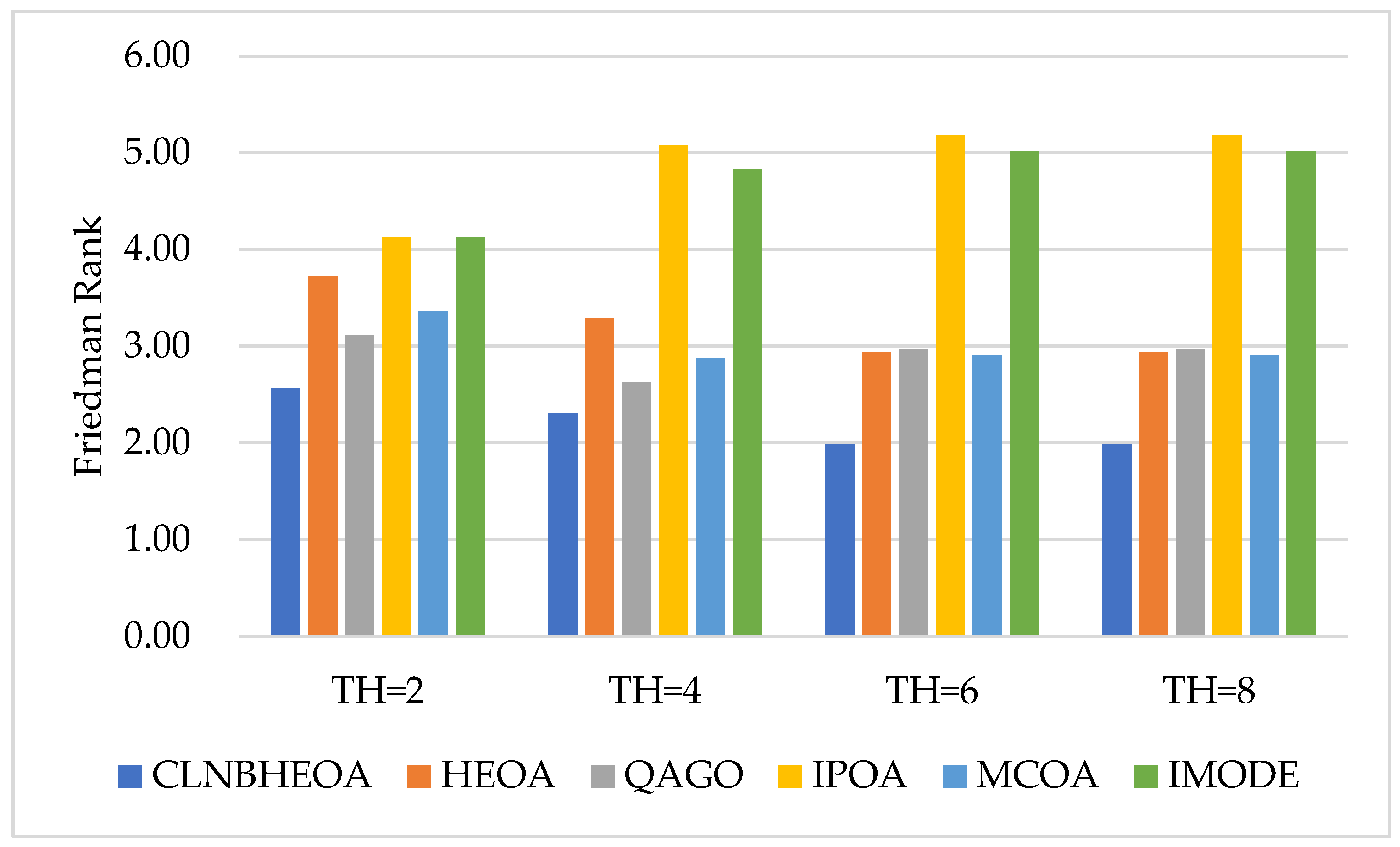
| Friedman Rank | 1.62 | 2.88 | 2.25 | 5.35 | 3.49 | 5.42 | |||||||
| Final Rank | 1.00 | 3.00 | 2.00 | 5.00 | 4.00 | 6.00 | |||||||
| Image | TH | CLNBHEOA | HEOA | QAGO | IPOA | MCOA | IMODE | ||||||
|---|---|---|---|---|---|---|---|---|---|---|---|---|---|
| Mean | Std | Mean | Std | Mean | Std | Mean | Std | Mean | Std | Mean | Std | ||
| Hunter | 2 | 1.79 × 10+01 | 0.00 × 10+00 | 1.78 × 10+01 | 4.35 × 10−01 | 1.79 × 10+01 | 7.95 × 10−03 | 1.72 × 10+01 | 1.31 × 10+00 | 1.79 × 10+01 | 3.17 × 10−01 | 1.76 × 10+01 | 4.10 × 10−01 |
| 4 | 2.22 × 10+01 | 3.14 × 10−02 | 2.20 × 10+01 | 6.15 × 10−01 | 2.21 × 10+01 | 5.00 × 10−02 | 2.00 × 10+01 | 2.76 × 10+00 | 2.20 × 10+01 | 2.80 × 10−01 | 2.07 × 10+01 | 7.56 × 10−01 | |
| 6 | 2.51 × 10+01 | 3.04 × 10−02 | 2.46 × 10+01 | 7.25 × 10−01 | 2.50 × 10+01 | 2.37 × 10−01 | 2.06 × 10+01 | 3.65 × 10+00 | 2.45 × 10+01 | 4.44 × 10−01 | 2.26 × 10+01 | 9.21 × 10−01 | |
| 8 | 2.68 × 10+01 | 9.58 × 10−02 | 2.64 × 10+01 | 7.74 × 10−01 | 2.67 × 10+01 | 1.42 × 10−01 | 2.37 × 10+01 | 1.17 × 10+00 | 2.64 × 10+01 | 2.6 × 10−01 | 2.37 × 10+01 | 9.70 × 10−01 | |
| Baboon | 2 | 1.53 × 10+01 | 5.47 × 10⁻¹⁵ | 1.52 × 10+01 | 0.00 × 10+00 | 1.52 × 10+01 | 4.07 × 10−02 | 1.47 × 10+01 | 1.30 × 10+00 | 1.52 × 10+01 | 4.47 × 10−01 | 1.49 × 10+01 | 1.22 × 10+00 |
| 4 | 2.05 × 10+01 | 4.10 × 10−02 | 1.98 × 10+01 | 1.86 × 10+00 | 2.04 × 10+01 | 9.46 × 10−02 | 1.80 × 10+01 | 3.10 × 10+00 | 2.02 × 10+01 | 7.08 × 10−01 | 1.84 × 10+01 | 1.54 × 10+00 | |
| 6 | 2.37 × 10+01 | 1.78 × 10−01 | 2.35 × 10+01 | 1.11 × 10+00 | 2.34 × 10+01 | 3.54 × 10−01 | 2.00 × 10+01 | 3.18 × 10+00 | 2.35 × 10+01 | 6.14 × 10−01 | 2.12 × 10+01 | 1.74 × 10+00 | |
| 8 | 2.63 × 10+01 | 4.80 × 10−01 | 2.54 × 10+01 | 2.03 × 10+00 | 2.61 × 10+01 | 2.96 × 10−01 | 2.07 × 10+01 | 4.04 × 10+00 | 2.62 × 10+01 | 3.44 × 10−01 | 2.25 × 10+01 | 1.74 × 10+00 | |
| Barbara | 2 | 1.64 × 10+01 | 1.88 × 10−02 | 1.63 × 10+01 | 5.67 × 10−01 | 1.63 × 10+01 | 3.65 × 10⁻¹⁵ | 1.54 × 10+01 | 1.86 × 10+00 | 1.62 × 10+01 | 6.63 × 10−01 | 1.56 × 10+01 | 7.99 × 10−01 |
| 4 | 1.98 × 10+01 | 2.33 × 10−01 | 1.92 × 10+01 | 1.35 × 10+00 | 1.96 × 10+01 | 9.48 × 10−02 | 1.87 × 10+01 | 1.00 × 10+00 | 1.97 × 10+01 | 3.52 × 10−02 | 1.86 × 10+01 | 1.19 × 10+00 | |
| 6 | 2.24 × 10+01 | 3.20 × 10−01 | 2.21 × 10+01 | 1.07 × 10+00 | 2.23 × 10+01 | 1.84 × 10−01 | 1.99 × 10+01 | 1.84 × 10+00 | 2.23 × 10+01 | 1.24 × 10−01 | 2.06 × 10+01 | 1.05 × 10+00 | |
| 8 | 2.43 × 10+01 | 2.23 × 10−01 | 2.33 × 10+01 | 1.73 × 10+00 | 2.41 × 10+01 | 1.45 × 10−01 | 2.19 × 10+01 | 1.55 × 10+00 | 2.42 × 10+01 | 2.17 × 10−01 | 2.24 × 10+01 | 1.27 × 10+00 | |
| Camera | 2 | 1.54 × 10+01 | 1.08 × 10+00 | 1.49 × 10+01 | 0.00 × 10+00 | 1.50 × 10+01 | 3.67 × 10−02 | 1.50 × 10+01 | 0.00 × 10+00 | 1.50 × 10+01 | 5.03 × 10−01 | 1.49 × 10+01 | 7.56 × 10−01 |
| 4 | 2.05 × 10+01 | 6.69 × 10−02 | 2.00 × 10+01 | 1.28 × 10+00 | 2.01 × 10+01 | 8.26 × 10−02 | 1.83 × 10+01 | 2.48 × 10+00 | 2.02 × 10+01 | 7.56 × 10−01 | 1.95 × 10+01 | 1.10 × 10+00 | |
| 6 | 2.34 × 10+01 | 2.33 × 10−01 | 2.21 × 10+01 | 1.86 × 10+00 | 2.31 × 10+01 | 3.52 × 10−01 | 2.10 × 10+01 | 1.95 × 10+00 | 2.27 × 10+01 | 4.35 × 10−01 | 2.10 × 10+01 | 1.09 × 10+00 | |
| 8 | 2.57 × 10+01 | 3.57 × 10−01 | 2.47 × 10+01 | 1.55 × 10+00 | 2.54 × 10+01 | 4.20 × 10−01 | 2.20 × 10+01 | 1.75 × 10+00 | 2.50 × 10+01 | 6.05 × 10−01 | 2.27 × 10+01 | 1.00 × 10+00 | |
| Lena | 2 | 1.54 × 10+01 | 1.82 × 10⁻¹⁵ | 1.53 × 10+01 | 1.82 × 10⁻¹⁵ | 1.53 × 10+01 | 2.61 × 10−02 | 1.41 × 10+01 | 1.59 × 10+00 | 1.52 × 10+01 | 4.67 × 10−01 | 1.44 × 10+01 | 8.25 × 10−01 |
| 4 | 1.86 × 10+01 | 2.55 × 10−02 | 1.81 × 10+01 | 1.11 × 10+00 | 1.87 × 10+01 | 2.98 × 10−02 | 1.79 × 10+01 | 1.13 × 10+00 | 1.85 × 10+01 | 3.42 × 10−01 | 1.78 × 10+01 | 8.79 × 10−01 | |
| 6 | 2.08 × 10+01 | 1.70 × 10−01 | 2.05 × 10+01 | 8.75 × 10−01 | 2.07 × 10+01 | 9.41 × 10−02 | 1.97 × 10+01 | 1.68 × 10+00 | 2.07 × 10+01 | 6.10 × 10−01 | 2.01 × 10+01 | 1.22 × 10+00 | |
| 8 | 2.33 × 10+01 | 5.92 × 10−01 | 2.28 × 10+01 | 1.62 × 10+00 | 2.27 × 10+01 | 8.34 × 10−01 | 1.99 × 10+01 | 3.11 × 10+00 | 2.30 × 10+01 | 8.21 × 10−01 | 2.17 × 10+01 | 1.11 × 10+00 | |
| Woman | 2 | 1.47 × 10+01 | 8.75 × 10−01 | 1.45 × 10+01 | 3.53 × 10−01 | 1.46 × 10+01 | 4.33 × 10−02 | 1.45 × 10+01 | 5.49 × 10−01 | 1.45 × 10+01 | 1.67 × 10−01 | 1.46 × 10+01 | 0.00 × 10+00 |
| 4 | 2.16 × 10+01 | 7.27 × 10−02 | 2.11 × 10+01 | 9.23 × 10−01 | 2.16 × 10+01 | 3.69 × 10−02 | 1.86 × 10+01 | 1.83 × 10+00 | 2.14 × 10+01 | 5.02 × 10−01 | 1.96 × 10+01 | 1.56 × 10+00 | |
| 6 | 2.39 × 10+01 | 1.15 × 10−01 | 2.33 × 10+01 | 7.01 × 10−01 | 2.37 × 10+01 | 3.31 × 10−01 | 2.05 × 10+01 | 2.40 × 10+00 | 2.40 × 10+01 | 7.79 × 10−01 | 2.10 × 10+01 | 1.61 × 10+00 | |
| 8 | 2.71 × 10+01 | 1.15 × 10−01 | 2.64 × 10+01 | 1.34 × 10+00 | 2.70 × 10+01 | 1.31 × 10−01 | 2.14 × 10+01 | 3.48 × 10+00 | 2.66 × 10+01 | 5.06 × 10−01 | 2.31 × 10+01 | 1.68 × 10+00 | |
| Friedman Rank | 2.21 | 3.22 | 2.92 | 4.89 | 3.01 | 4.75 | |||||||
| Final Rank | 1 | 4 | 2 | 6 | 3 | 5 | |||||||
| Image | TH | CLNBHEOA | HEOA | QAGO | IPOA | MCOA | IMODE | ||||||
|---|---|---|---|---|---|---|---|---|---|---|---|---|---|
| Mean | Std | Mean | Std | Mean | Std | Mean | Std | Mean | Std | Mean | Std | ||
| Hunter | 2 | 7.89 × 10−01 | 5.37 × 10−03 | 7.61 × 10−01 | 4.39 × 10−03 | 7.61 × 10−01 | 5.64 × 10−03 | 7.58 × 10−01 | 5.86 × 10−03 | 7.60 × 10−01 | 6.18 × 10−03 | 7.63 × 10−01 | 5.09 × 10−03 |
| 4 | 8.31 × 10−01 | 6.04 × 10−03 | 8.05 × 10−01 | 2.18 × 10−03 | 8.03 × 10−01 | 2.21 × 10−03 | 8.06 × 10−01 | 2.24 × 10−03 | 8.03 × 10−01 | 2.19 × 10−03 | 8.04 × 10−01 | 2.34 × 10−03 | |
| 6 | 8.44 × 10−01 | 2.51 × 10−03 | 8.26 × 10−01 | 3.09 × 10−03 | 8.25 × 10−01 | 2.52 × 10−03 | 8.26 × 10−01 | 3.33 × 10−03 | 8.26 × 10−01 | 2.75 × 10−03 | 8.25 × 10−01 | 2.77 × 10−03 | |
| 8 | 8.59 × 10−01 | 6.34 × 10−03 | 8.38 × 10−01 | 6.09 × 10−03 | 8.38 × 10−01 | 5.98 × 10−03 | 8.39 × 10−01 | 6.33 × 10−03 | 8.39 × 10−01 | 6.39 × 10−03 | 8.40 × 10−01 | 5.07 × 10−03 | |
| Baboon | 2 | 7.83 × 10−01 | 8.90 × 10−03 | 7.55 × 10−01 | 2.61 × 10−03 | 7.55 × 10−01 | 2.71 × 10−03 | 7.55 × 10−01 | 2.86 × 10−03 | 7.55 × 10−01 | 2.93 × 10−03 | 7.55 × 10−01 | 2.82 × 10−03 |
| 4 | 8.22 × 10−01 | 5.58 × 10−03 | 8.05 × 10−01 | 3.13 × 10−03 | 8.04 × 10−01 | 2.67 × 10−03 | 8.06 × 10−01 | 2.87 × 10−03 | 8.05 × 10−01 | 2.70 × 10−03 | 8.05 × 10−01 | 3.18 × 10−03 | |
| 6 | 8.74 × 10−01 | 2.20 × 10−03 | 8.65 × 10−01 | 3.03 × 10−02 | 8.69 × 10−01 | 5.15 × 10−03 | 7.45 × 10−01 | 1.32 × 10−01 | 8.65 × 10−01 | 1.31 × 10−02 | 7.99 × 10−01 | 4.76 × 10−02 | |
| 8 | 9.16 × 10−01 | 5.31 × 10−03 | 8.91 × 10−01 | 4.99 × 10−02 | 9.15 × 10−01 | 2.85 × 10−03 | 7.48 × 10−01 | 1.69 × 10−01 | 9.13 × 10−01 | 5.23 × 10−03 | 8.31 × 10−01 | 4.12 × 10−02 | |
| Barbara | 2 | 7.81 × 10−01 | 5.76 × 10−03 | 7.55 × 10−01 | 3.64 × 10−03 | 7.54 × 10−01 | 2.84 × 10−03 | 7.56 × 10−01 | 3.18 × 10−03 | 7.55 × 10−01 | 2.79 × 10−03 | 7.55 × 10−01 | 3.04 × 10−03 |
| 4 | 8.22 × 10−01 | 5.97 × 10−03 | 8.05 × 10−01 | 2.95 × 10−03 | 8.05 × 10−01 | 3.18 × 10−03 | 8.06 × 10−01 | 3.31 × 10−03 | 8.04 × 10−01 | 2.48 × 10−03 | 8.05 × 10−01 | 3.53 × 10−03 | |
| 6 | 8.40 × 10−01 | 5.05 × 10−03 | 8.25 × 10−01 | 2.79 × 10−03 | 8.26 × 10−01 | 2.77 × 10−03 | 8.19 × 10−01 | 3.62 × 10−02 | 8.25 × 10−01 | 3.23 × 10−03 | 8.25 × 10−01 | 3.26 × 10−03 | |
| 8 | 8.60 × 10−01 | 5.42 × 10−03 | 8.42 × 10−01 | 6.39 × 10−03 | 8.40 × 10−01 | 6.26 × 10−03 | 8.39 × 10−01 | 5.76 × 10−03 | 8.40 × 10−01 | 6.53 × 10−03 | 8.42 × 10−01 | 5.76 × 10−03 | |
| Camera | 2 | 7.95 × 10−01 | 3.02 × 10−03 | 7.61 × 10−01 | 5.03 × 10−03 | 7.59 × 10−01 | 6.45 × 10−03 | 7.59 × 10−01 | 5.60 × 10−03 | 7.60 × 10−01 | 5.72 × 10−03 | 7.59 × 10−01 | 5.97 × 10−03 |
| 4 | 8.30 × 10−01 | 5.98 × 10−03 | 8.11 × 10−01 | 6.26 × 10−03 | 8.08 × 10−01 | 6.20 × 10−03 | 8.09 × 10−01 | 5.62 × 10−03 | 8.08 × 10−01 | 5.98 × 10−03 | 8.10 × 10−01 | 5.83 × 10−03 | |
| 6 | 8.46 × 10−01 | 2.36 × 10−03 | 8.25 × 10−01 | 2.74 × 10−03 | 8.25 × 10−01 | 3.19 × 10−03 | 8.25 × 10−01 | 2.92 × 10−03 | 8.25 × 10−01 | 3.04 × 10−03 | 8.25 × 10−01 | 3.08 × 10−03 | |
| 8 | 8.59 × 10−01 | 6.04 × 10−03 | 8.35 × 10−01 | 2.70 × 10−03 | 8.34 × 10−01 | 2.73 × 10−03 | 8.35 × 10−01 | 2.93 × 10−03 | 8.35 × 10−01 | 2.71 × 10−03 | 8.35 × 10−01 | 2.48 × 10−03 | |
| Lena | 2 | 7.94 × 10−01 | 3.23 × 10−03 | 7.90 × 10−01 | 6.11 × 10−03 | 7.92 × 10−01 | 5.92 × 10−03 | 7.78 × 10−01 | 5.68 × 10−02 | 7.91 × 10−01 | 6.12 × 10−03 | 7.89 × 10−01 | 6.46 × 10−03 |
| 4 | 8.30 × 10−01 | 7.12 × 10−03 | 8.07 × 10−01 | 6.06 × 10−03 | 8.10 × 10−01 | 6.71 × 10−03 | 8.10 × 10−01 | 5.71 × 10−03 | 8.08 × 10−01 | 5.90 × 10−03 | 8.13 × 10−01 | 5.63 × 10−03 | |
| 6 | 8.44 × 10−01 | 2.72 × 10−03 | 8.25 × 10−01 | 2.48 × 10−03 | 8.26 × 10−01 | 2.98 × 10−03 | 8.25 × 10−01 | 2.87 × 10−03 | 8.24 × 10−01 | 2.57 × 10−03 | 8.25 × 10−01 | 3.15 × 10−03 | |
| 8 | 8.63 × 10−01 | 6.11 × 10−03 | 8.41 × 10−01 | 5.48 × 10−03 | 8.41 × 10−01 | 5.62 × 10−03 | 8.39 × 10−01 | 6.16 × 10−03 | 8.41 × 10−01 | 6.57 × 10−03 | 8.40 × 10−01 | 6.39 × 10−03 | |
| Woman | 2 | 7.95 × 10−01 | 2.86 × 10−03 | 7.64 × 10−01 | 8.70 × 10−03 | 7.66 × 10−01 | 9.26 × 10−03 | 7.66 × 10−01 | 8.17 × 10−03 | 7.65 × 10−01 | 8.74 × 10−03 | 7.63 × 10−01 | 9.42 × 10−03 |
| 4 | 8.31 × 10−01 | 4.93 × 10−03 | 8.09 × 10−01 | 6.62 × 10−03 | 8.11 × 10−01 | 6.13 × 10−03 | 8.11 × 10−01 | 6.98 × 10−03 | 8.10 × 10−01 | 5.87 × 10−03 | 8.11 × 10−01 | 6.84 × 10−03 | |
| 6 | 8.45 × 10−01 | 2.78 × 10−03 | 8.24 × 10−01 | 2.97 × 10−03 | 8.25 × 10−01 | 2.98 × 10−03 | 8.24 × 10−01 | 3.17 × 10−03 | 8.25 × 10−01 | 2.60 × 10−03 | 8.26 × 10−01 | 2.96 × 10−03 | |
| 8 | 8.93 × 10−01 | 3.90 × 10−03 | 8.65 × 10−01 | 3.00 × 10−03 | 8.64 × 10−01 | 2.87 × 10−03 | 8.66 × 10−01 | 3.09 × 10−03 | 8.65 × 10−01 | 3.22 × 10−03 | 8.66 × 10−01 | 3.31 × 10−03 | |
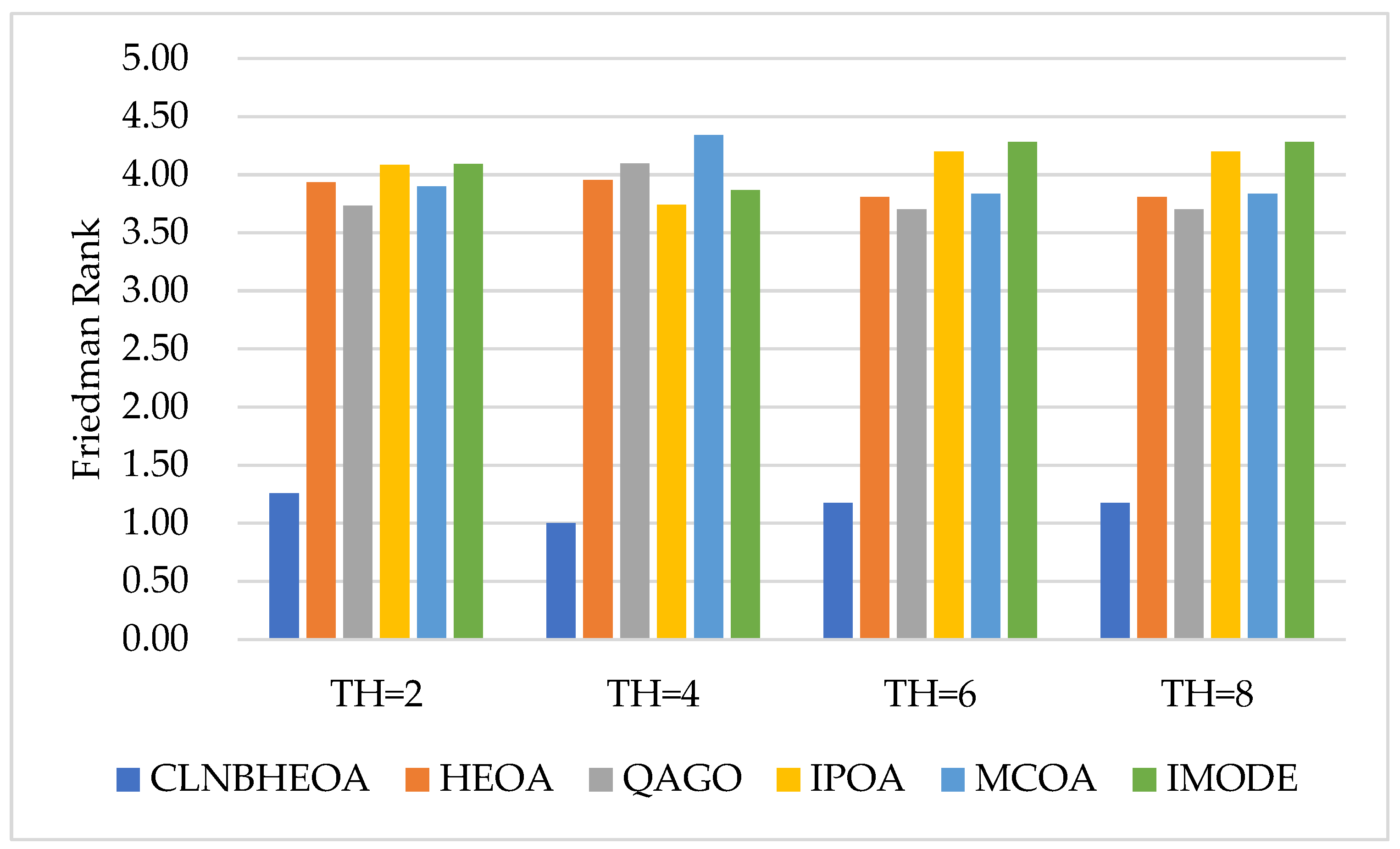
| Friedman Rank | 1.15 | 3.88 | 3.81 | 4.06 | 3.98 | 4.13 | |||||||
| Final Rank | 1 | 3 | 2 | 5 | 4 | 6 | |||||||
| Image | TH | CLNBHEOA | HEOA | QAGO | IPOA | MCOA | IMODE | ||||||
|---|---|---|---|---|---|---|---|---|---|---|---|---|---|
| Mean | Std | Mean | Std | Mean | Std | Mean | Std | Mean | Std | Mean | Std | ||
| Hunter | 2 | 7.96 × 10−01 | 3.04 × 10−03 | 7.67 × 10−01 | 1.45 × 10−02 | 7.68 × 10−01 | 1.35 × 10−02 | 7.69 × 10−01 | 1.32 × 10−02 | 7.67 × 10−01 | 1.35 × 10−02 | 7.67 × 10−01 | 1.76 × 10−02 |
| 4 | 8.54 × 10−01 | 2.28 × 10−04 | 8.46 × 10−01 | 1.98 × 10−02 | 8.52 × 10−01 | 1.71 × 10−03 | 7.89 × 10−01 | 8.94 × 10−02 | 8.49 × 10−01 | 6.68 × 10−03 | 8.13 × 10−01 | 1.76 × 10−02 | |
| 6 | 9.09 × 10−01 | 3.70 × 10−04 | 9.00 × 10−01 | 1.69 × 10−02 | 9.07 × 10−01 | 1.56 × 10−03 | 8.06 × 10−01 | 9.06 × 10−02 | 9.01 × 10−01 | 6.85 × 10−03 | 8.54 × 10−01 | 2.19 × 10−02 | |
| 8 | 9.39 × 10−01 | 4.39 × 10−04 | 9.34 × 10−01 | 1.67 × 10−02 | 9.38 × 10−01 | 1.69 × 10−03 | 8.79 × 10−01 | 2.76 × 10−02 | 9.35 × 10−01 | 5.54 × 10−03 | 8.86 × 10−01 | 1.75 × 10−02 | |
| Baboon | 2 | 7.95 × 10−01 | 2.61 × 10−03 | 7.64 × 10−01 | 1.47 × 10−02 | 7.67 × 10−01 | 1.63 × 10−02 | 7.68 × 10−01 | 1.32 × 10−02 | 7.68 × 10−01 | 1.58 × 10−02 | 7.61 × 10−01 | 1.68 × 10−02 |
| 4 | 8.43 × 10−01 | 8.85 × 10−04 | 8.16 × 10−01 | 6.17 × 10−02 | 8.42 × 10−01 | 1.75 × 10−03 | 7.69 × 10−01 | 1.11 × 10−01 | 8.35 × 10−01 | 1.82 × 10−02 | 7.82 × 10−01 | 4.18 × 10−02 | |
| 6 | 8.99 × 10−01 | 2.85 × 10−03 | 8.93 × 10−01 | 2.38 × 10−02 | 8.96 × 10−01 | 3.64 × 10−03 | 8.08 × 10−01 | 1.01 × 10−01 | 8.95 × 10−01 | 1.26 × 10−02 | 8.51 × 10−01 | 3.48 × 10−02 | |
| 8 | 9.34 × 10−01 | 6.87 × 10−03 | 9.17 × 10−01 | 3.76 × 10−02 | 9.34 × 10−01 | 4.81 × 10−03 | 8.09 × 10−01 | 1.29 × 10−01 | 9.34 × 10−01 | 5.48 × 10−03 | 8.73 × 10−01 | 3.66 × 10−02 | |
| Barbara | 2 | 7.85 × 10−01 | 2.13 × 10−03 | 7.61 × 10−01 | 7.18 × 10−03 | 7.66 × 10−01 | 8.16 × 10−03 | 7.64 × 10−01 | 8.73 × 10−03 | 7.65 × 10−01 | 1.48 × 10−02 | 7.66 × 10−01 | 8.71 × 10−03 |
| 4 | 8.07 × 10−01 | 6.96 × 10−04 | 7.89 × 10−01 | 3.32 × 10−02 | 8.07 × 10−01 | 6.93 × 10−04 | 7.74 × 10−01 | 2.36 × 10−02 | 8.06 × 10−01 | 2.64 × 10−03 | 7.68 × 10−01 | 2.75 × 10−02 | |
| 6 | 8.63 × 10−01 | 1.41 × 10−03 | 8.56 × 10−01 | 2.38 × 10−02 | 8.62 × 10−01 | 1.11 × 10−03 | 7.85 × 10−01 | 4.40 × 10−02 | 8.58 × 10−01 | 7.46 × 10−03 | 8.05 × 10−01 | 1.97 × 10−02 | |
| 8 | 8.93 × 10−01 | 7.43 × 10−04 | 8.67 × 10−01 | 3.89 × 10−02 | 8.92 × 10−01 | 1.08 × 10−03 | 8.28 × 10−01 | 3.12 × 10−02 | 8.92 × 10−01 | 2.84 × 10−03 | 8.47 × 10−01 | 1.49 × 10−02 | |
| Camera | 2 | 7.85 × 10−01 | 3.06 × 10−03 | 7.65 × 10−01 | 8.23 × 10−03 | 7.69 × 10−01 | 8.25 × 10−03 | 7.64 × 10−01 | 7.83 × 10−03 | 7.64 × 10−01 | 9.72 × 10−03 | 7.60 × 10−01 | 8.44 × 10−03 |
| 4 | 8.28 × 10−01 | 1.20 × 10−03 | 8.17 × 10−01 | 2.81 × 10−02 | 8.27 × 10−01 | 1.09 × 10−03 | 7.93 × 10−01 | 3.17 × 10−02 | 8.18 × 10−01 | 2.07 × 10−02 | 7.93 × 10−01 | 2.08 × 10−02 | |
| 6 | 8.74 × 10−01 | 1.33 × 10−02 | 8.46 × 10−01 | 3.89 × 10−02 | 8.73 × 10−01 | 7.82 × 10−03 | 8.33 × 10−01 | 4.48 × 10−02 | 8.66 × 10−01 | 1.53 × 10−02 | 8.31 × 10−01 | 2.48 × 10−02 | |
| 8 | 9.13 × 10−01 | 3.20 × 10−03 | 9.01 × 10−01 | 2.20 × 10−02 | 9.12 × 10−01 | 3.48 × 10−03 | 8.57 × 10−01 | 2.12 × 10−02 | 9.03 × 10−01 | 1.02 × 10−02 | 8.74 × 10−01 | 1.69 × 10−02 | |
| Lena | 2 | 7.91 × 10−01 | 5.97 × 10−03 | 7.64 × 10−01 | 8.86 × 10−03 | 7.60 × 10−01 | 7.93 × 10−03 | 7.65 × 10−01 | 7.98 × 10−03 | 7.64 × 10−01 | 8.87 × 10−03 | 7.65 × 10−01 | 8.40 × 10−03 |
| 4 | 8.28 × 10−01 | 5.54 × 10−03 | 8.13 × 10−01 | 5.33 × 10−03 | 8.10 × 10−01 | 6.83 × 10−03 | 8.08 × 10−01 | 5.34 × 10−03 | 8.08 × 10−01 | 5.53 × 10−03 | 8.10 × 10−01 | 4.89 × 10−03 | |
| 6 | 8.53 × 10−01 | 8.15 × 10−04 | 8.42 × 10−01 | 2.33 × 10−02 | 8.52 × 10−01 | 8.29 × 10−04 | 7.99 × 10−01 | 3.39 × 10−02 | 8.44 × 10−01 | 1.05 × 10−02 | 8.02 × 10−01 | 2.02 × 10−02 | |
| 8 | 8.71 × 10−01 | 2.33 × 10−03 | 8.63 × 10−01 | 2.08 × 10−02 | 8.70 × 10−01 | 1.50 × 10−03 | 8.02 × 10−01 | 5.88 × 10−02 | 8.67 × 10−01 | 3.98 × 10−03 | 8.34 × 10−01 | 1.62 × 10−02 | |
| Woman | 2 | 7.94 × 10−01 | 2.56 × 10−03 | 7.75 × 10−01 | 2.92 × 10−03 | 7.74 × 10−01 | 2.58 × 10−03 | 7.75 × 10−01 | 2.72 × 10−03 | 7.76 × 10−01 | 2.66 × 10−03 | 7.74 × 10−01 | 2.57 × 10−03 |
| 4 | 8.16 × 10−01 | 7.67 × 10−04 | 8.05 × 10−01 | 2.28 × 10−02 | 8.15 × 10−01 | 9.54 × 10−04 | 7.50 × 10−01 | 2.51 × 10−02 | 8.08 × 10−01 | 1.30 × 10−02 | 7.86 × 10−01 | 1.79 × 10−02 | |
| 6 | 8.84 × 10−01 | 1.90 × 10−03 | 8.81 × 10−01 | 1.70 × 10−02 | 8.83 × 10−01 | 2.89 × 10−03 | 7.86 × 10−01 | 5.95 × 10−02 | 8.70 × 10−01 | 1.23 × 10−02 | 8.00 × 10−01 | 3.38 × 10−02 | |
| 8 | 9.17 × 10−01 | 1.86 × 10−03 | 9.05 × 10−01 | 3.04 × 10−02 | 9.16 × 10−01 | 1.76 × 10−03 | 7.99 × 10−01 | 7.89 × 10−02 | 9.07 × 10−01 | 9.87 × 10−03 | 8.37 × 10−01 | 3.21 × 10−02 | |
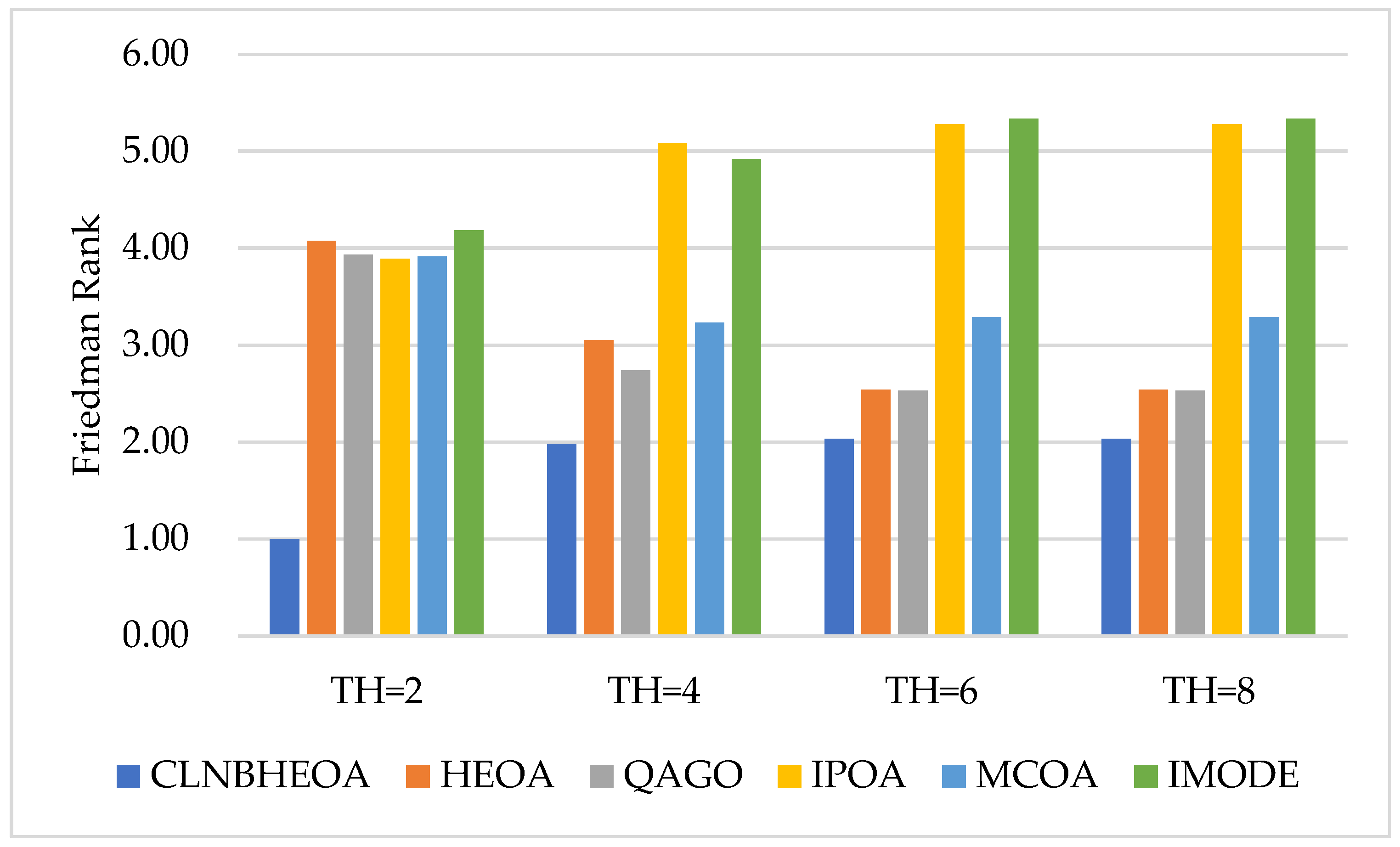
| Friedman Rank | 1.76 | 3.05 | 2.93 | 4.88 | 3.43 | 4.94 | |||||||
| Final Rank | 1 | 3 | 2 | 5 | 4 | 6 | |||||||
Disclaimer/Publisher’s Note: The statements, opinions and data contained in all publications are solely those of the individual author(s) and contributor(s) and not of MDPI and/or the editor(s). MDPI and/or the editor(s) disclaim responsibility for any injury to people or property resulting from any ideas, methods, instructions or products referred to in the content. |
© 2025 by the authors. Licensee MDPI, Basel, Switzerland. This article is an open access article distributed under the terms and conditions of the Creative Commons Attribution (CC BY) license (https://creativecommons.org/licenses/by/4.0/).
Share and Cite
Xiang, L.; Zhao, X.; Wang, J.; Wang, B. An Enhanced Human Evolutionary Optimization Algorithm for Global Optimization and Multi-Threshold Image Segmentation. Biomimetics 2025, 10, 282. https://doi.org/10.3390/biomimetics10050282
Xiang L, Zhao X, Wang J, Wang B. An Enhanced Human Evolutionary Optimization Algorithm for Global Optimization and Multi-Threshold Image Segmentation. Biomimetics. 2025; 10(5):282. https://doi.org/10.3390/biomimetics10050282
Chicago/Turabian StyleXiang, Liang, Xiajie Zhao, Jianfeng Wang, and Bin Wang. 2025. "An Enhanced Human Evolutionary Optimization Algorithm for Global Optimization and Multi-Threshold Image Segmentation" Biomimetics 10, no. 5: 282. https://doi.org/10.3390/biomimetics10050282
APA StyleXiang, L., Zhao, X., Wang, J., & Wang, B. (2025). An Enhanced Human Evolutionary Optimization Algorithm for Global Optimization and Multi-Threshold Image Segmentation. Biomimetics, 10(5), 282. https://doi.org/10.3390/biomimetics10050282