Figure 1.
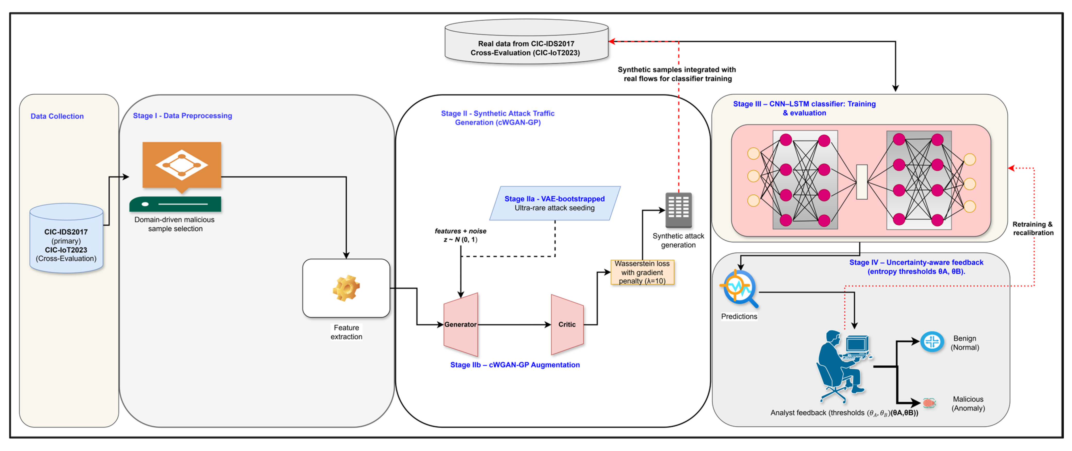
Proposed uncertainty-aware intrusion detection workflow. Stage I performs leakage-safe preprocessing on CIC-IDS2017 (primary) and CIC-IoT2023 (cross-evaluation), including domain-driven selection of minority attacks and feature extraction. Stage II introduces generative augmentation: (IIa) a variational autoencoder (VAE) bootstraps ultra-rare classes, and (IIb) a conditional Wasserstein GAN with gradient penalty (cWGAN-GP) synthesizes diverse attack flows that are merged with real traffic. Stage III involved training the calibrated CNN–LSTM classifier using the combined dataset. Stage IV applies entropy-based thresholds (θA, θB) to defer uncertain predictions to analysts; their feedback is logged for periodic retraining and recalibration.
Figure 2.
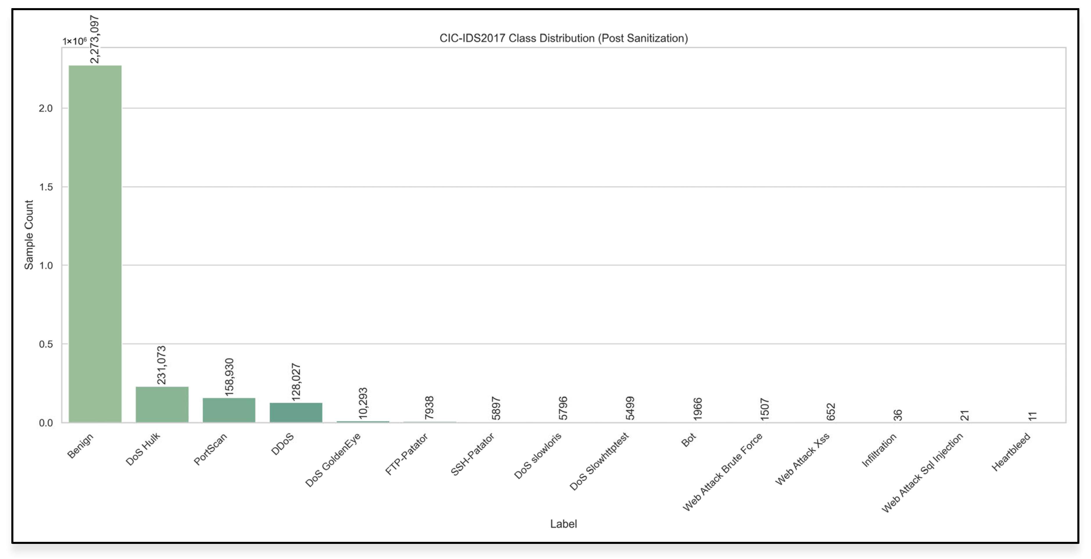
Class distribution of the CIC-IDS2017 dataset.
Figure 2.
Class distribution of the CIC-IDS2017 dataset.
Figure 3.
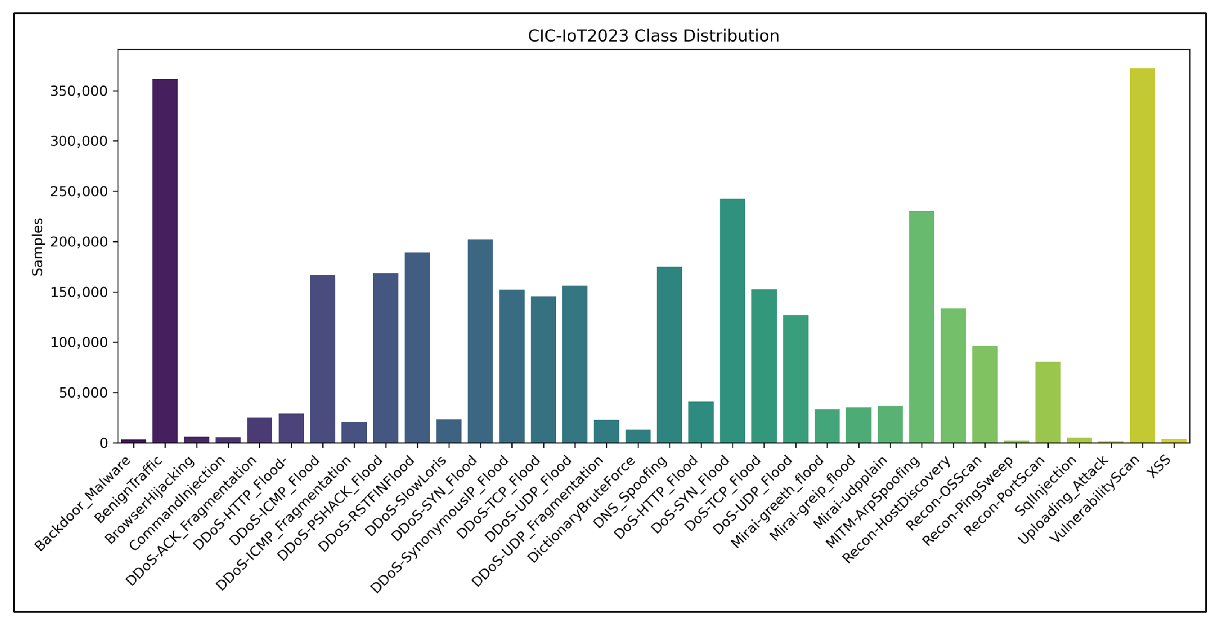
Class distribution of the CIC-IoT2023 dataset.
Figure 3.
Class distribution of the CIC-IoT2023 dataset.
Figure 4.
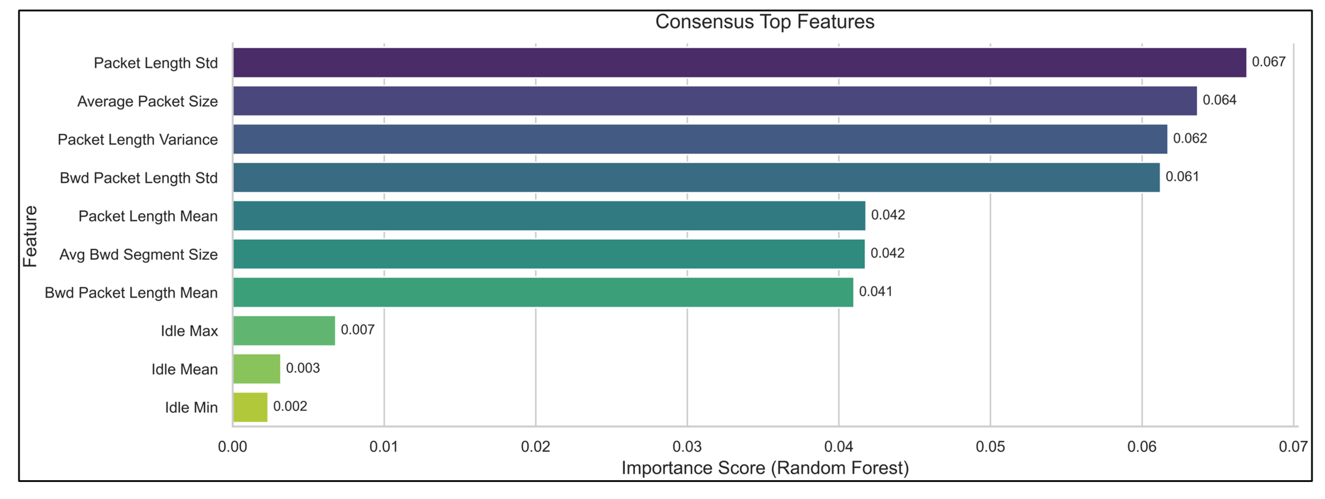
Consensus top flow features driving IDS decisions.
Figure 4.
Consensus top flow features driving IDS decisions.
Figure 5.
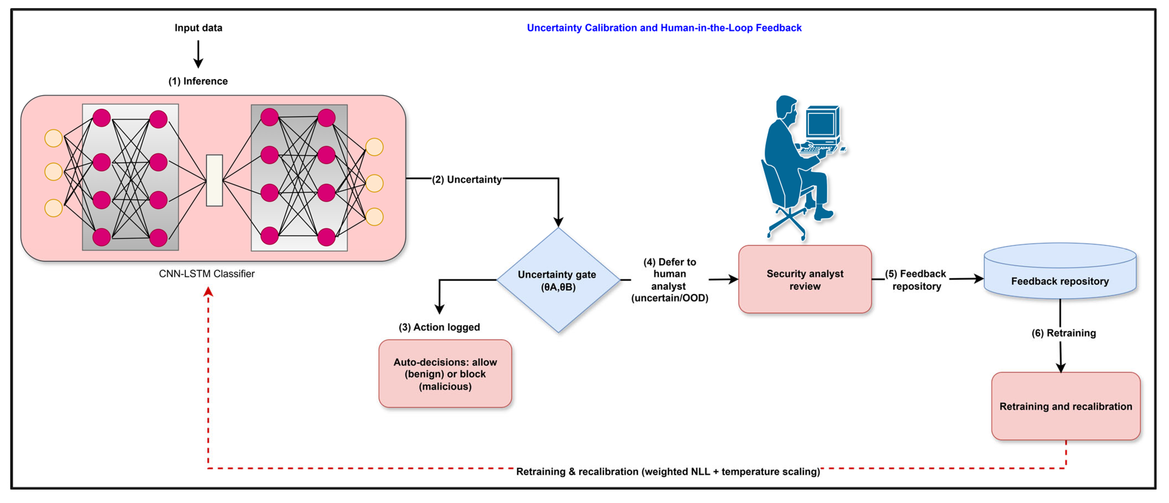
The uncertainty calibration and analysis feedback mechanisms are discussed. Predictions passing through the entropy-based uncertainty gate are either auto-decided (benign/malicious) or deferred to a human analyst for evaluation. Analyst feedback is stored in a repository and used for retraining and recalibration via weighted NLL and temperature-scaling.
Figure 6.
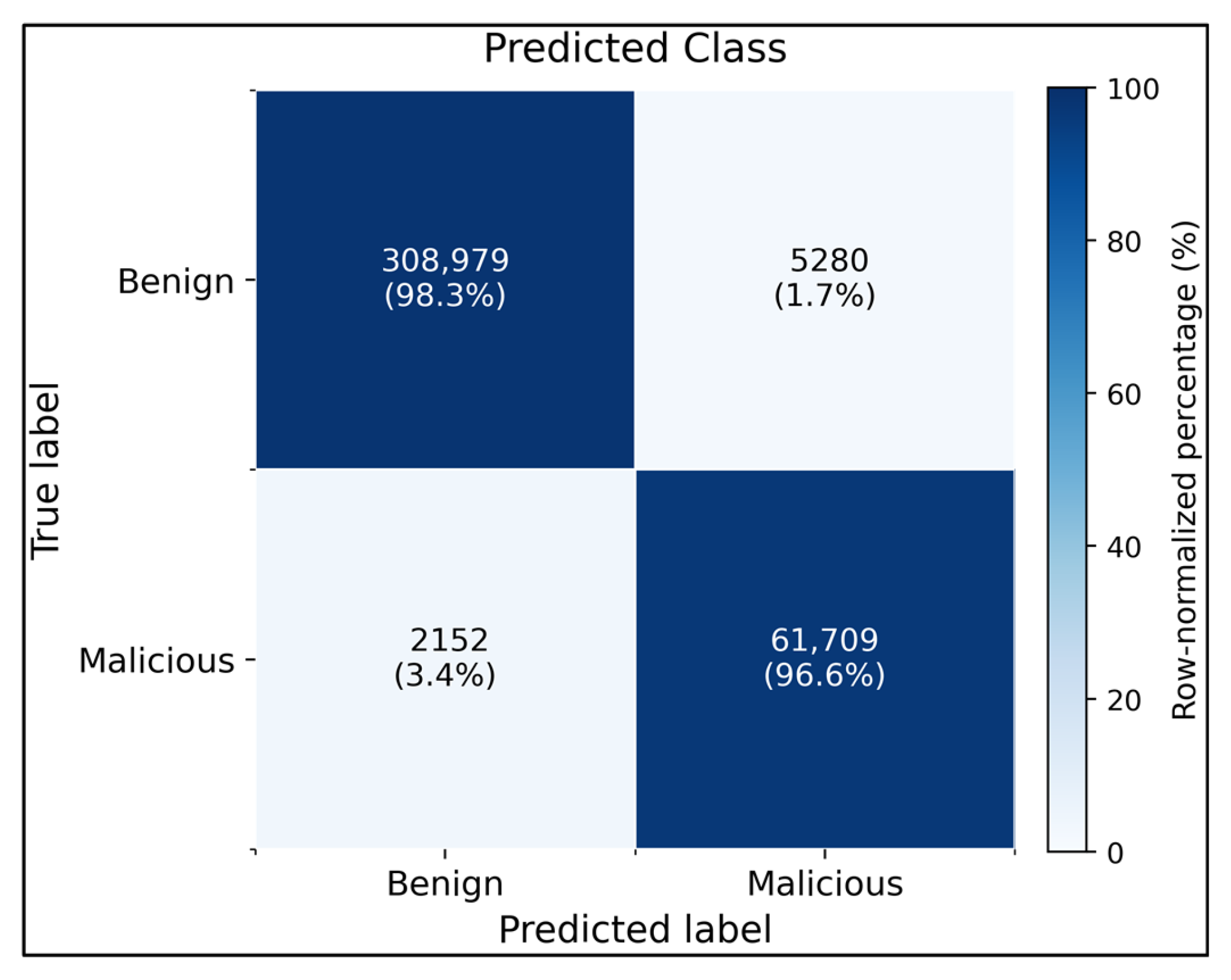
Binary confusion matrix for the baseline CNN–LSTM on the CIC-IDS2017 test split using all 46 features. The classifier correctly identified 98.3% of benign flows (308,979/314,259) and 96.6% of malicious flows (61,709/63,861), with only 1.7% false positives and 3.4% false negatives, demonstrating a high-fidelity benign–malicious separation.
Figure 7.
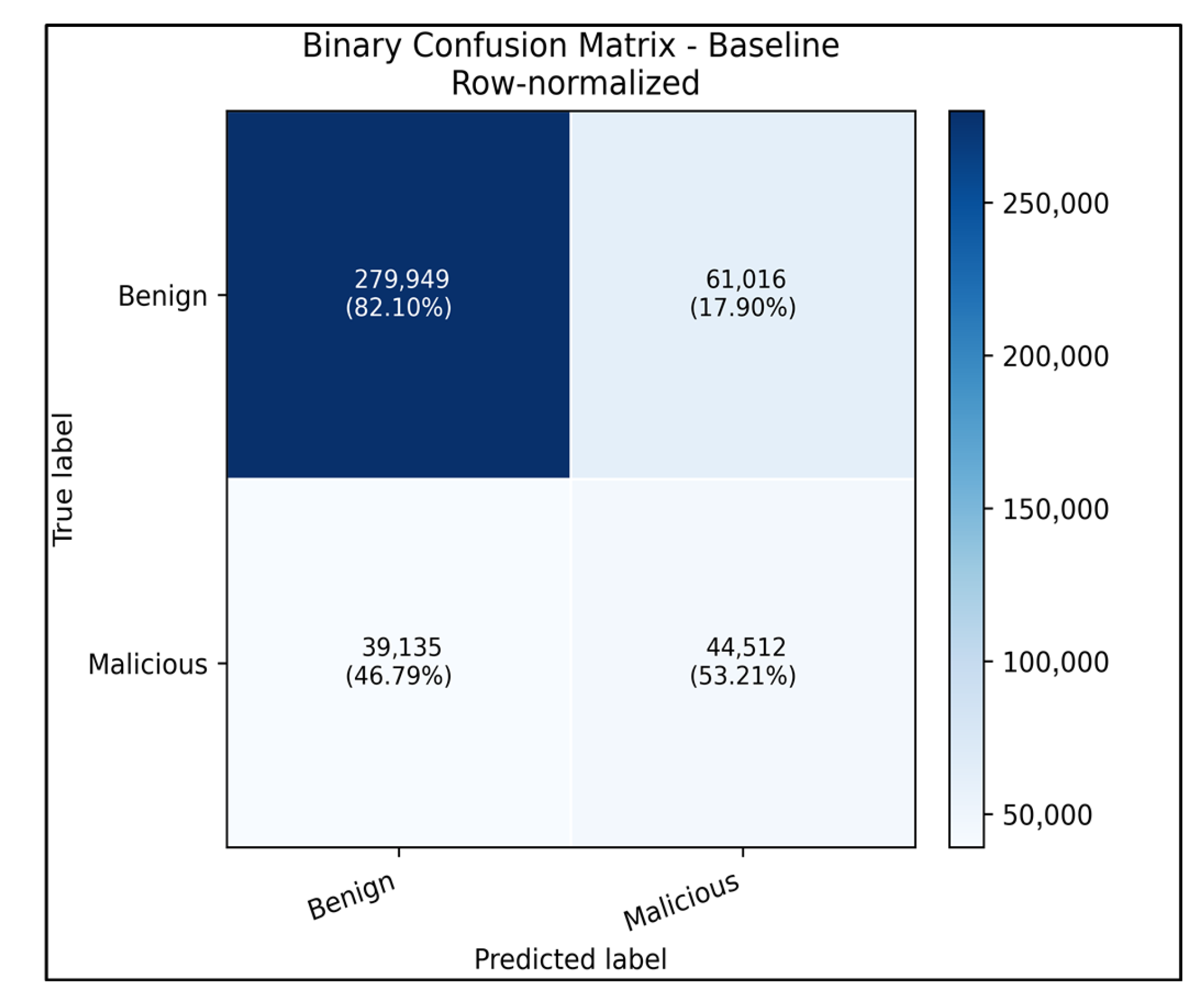
Row-normalized confusion matrix of the baseline binary CNN–LSTM evaluated on the CIC-IDS2017 dataset. Benign flows were correctly classified 82.1% of the time (17.9% false positives), whereas malicious flows reached 53.2% true positives with 46.8% missed detections, illustrating the remaining imbalance between benign and attack coverage even after calibration.
Figure 8.
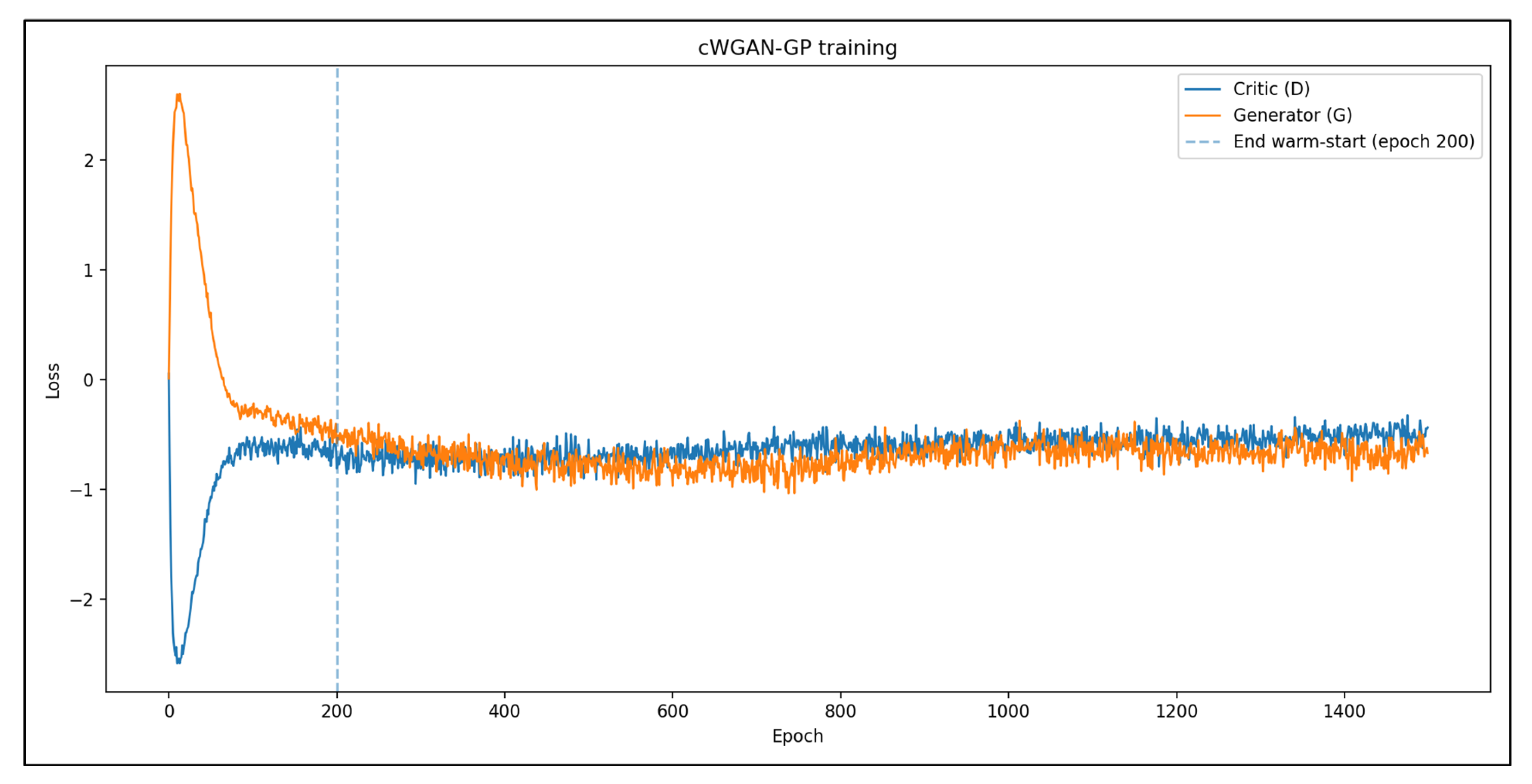
Training dynamics of the cWGAN-GP used for synthetic attack flow generation. The critic loss (blue) initially increased as the discriminator learned to distinguish between real and synthetic flows, and then stabilized with oscillatory behavior indicative of equilibrium. The generator loss (orange) gradually improved, reflecting the increased fidelity of the generated samples. The stable convergence pattern, with no mode collapse or divergence, validates the suitability of the cWGAN-GP for realistic network traffic synthesis in scenarios with imbalanced intrusion detection.
Figure 9.
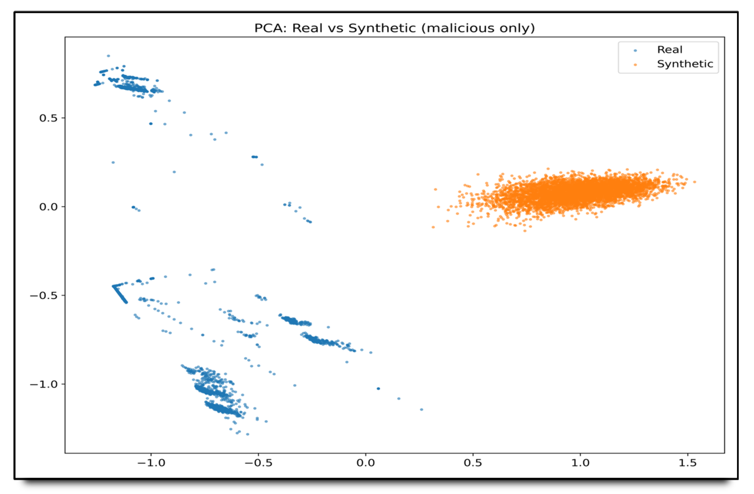
PCA visualization of real versus synthetic malicious flows. The 2D embedding reveals that real attack traces (blue) occupy a broader manifold, whereas cWGAN-GP samples (orange) cluster tightly, indicating a reduced intra-class diversity. This divergence underscores the need for additional regularization or conditioning to better match the variability of real-world attack behavior.
Figure 10.
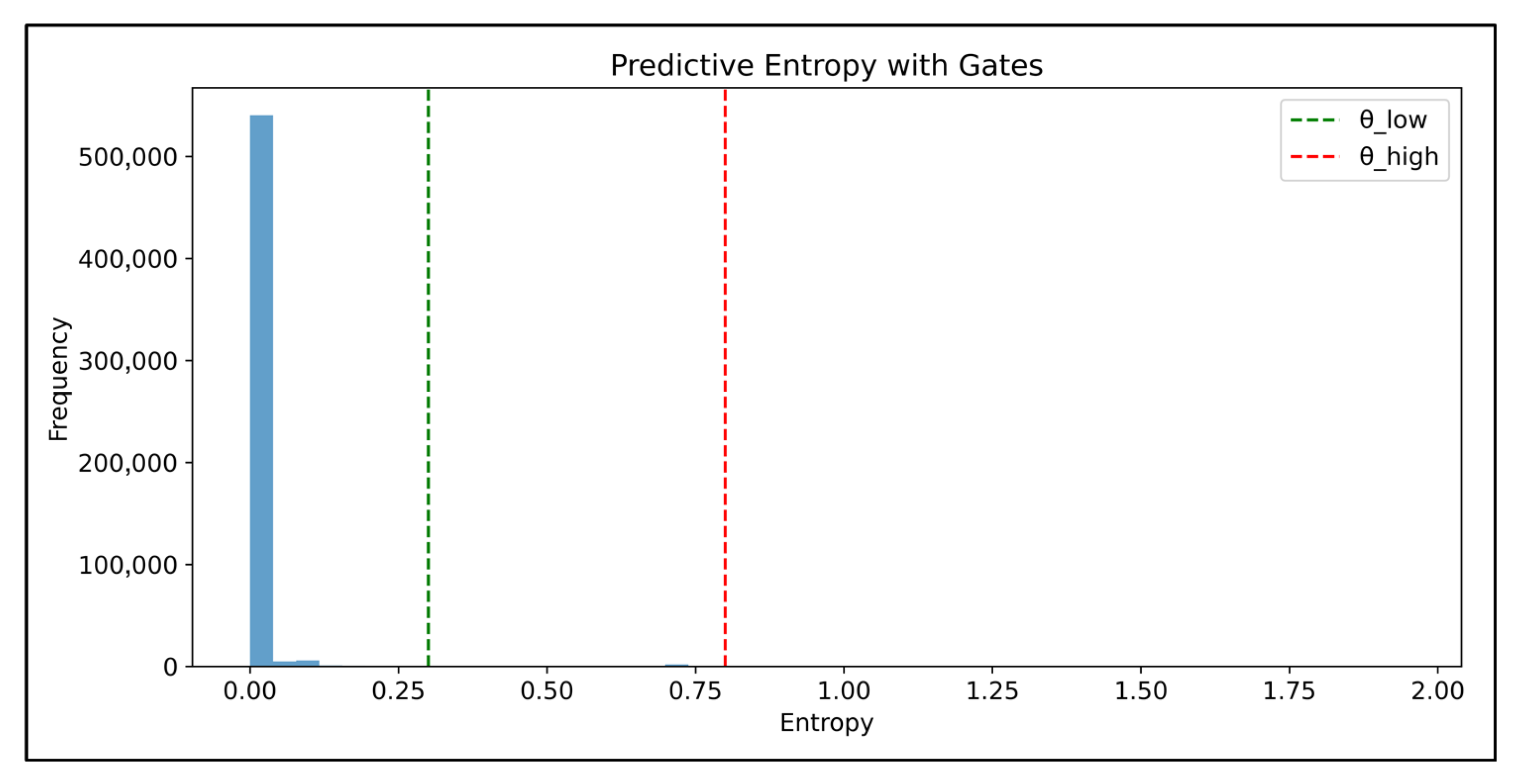
Predictive entropy distribution for the calibrated CNN–LSTM on CIC-IDS2017 (validation set) under the hu-man-in-the-loop gating policy. The dashed lines mark the low threshold (green) used for auto-acceptance and the high threshold (red), indicating high-confidence decisions, whereas only a small tail is routed to the feedback queue.
Figure 11.
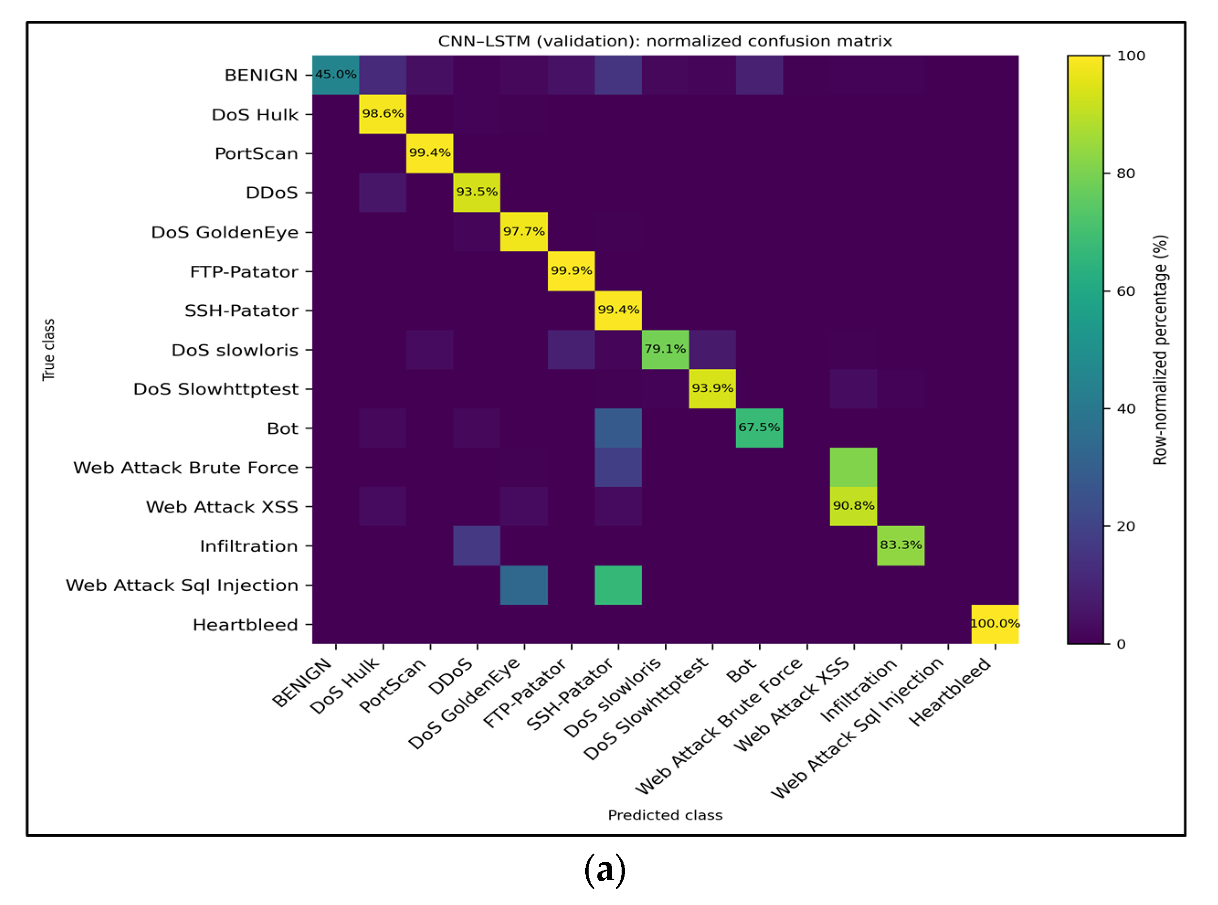
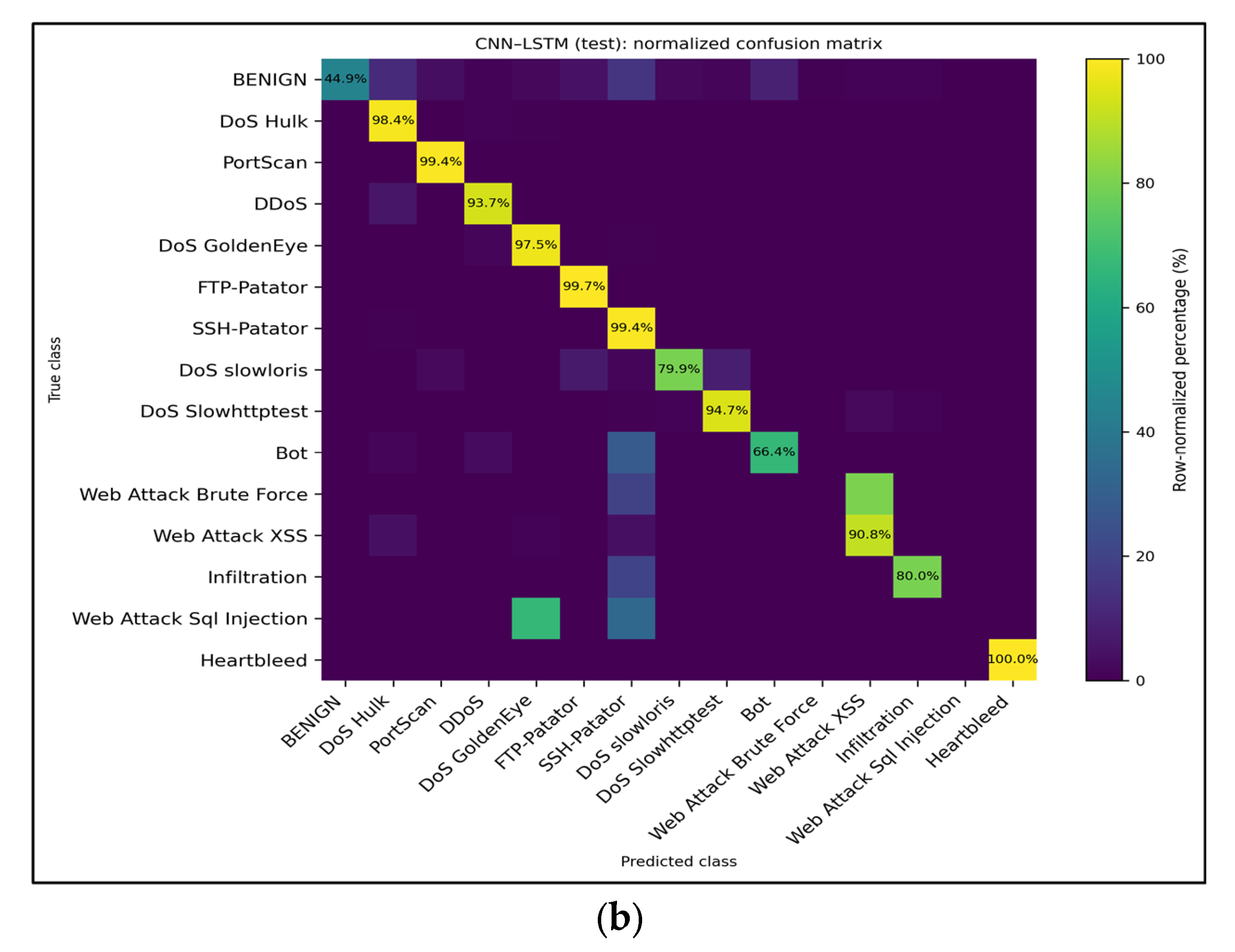
Row-normalized multiclass confusion matrices for the baseline CNN–LSTM model trained on all features. (a) Validation split—major high-volume attacks retain >97% recall, whereas minority classes, such as Web Attack–XSS and Infiltration, remain the primary sources of error. (b) Test split—shows nearly identical behavior, confirming that the multiclass performance generalizes across holds. The values inside each cell denote the recall percentages for the corresponding true class.
Figure 12.
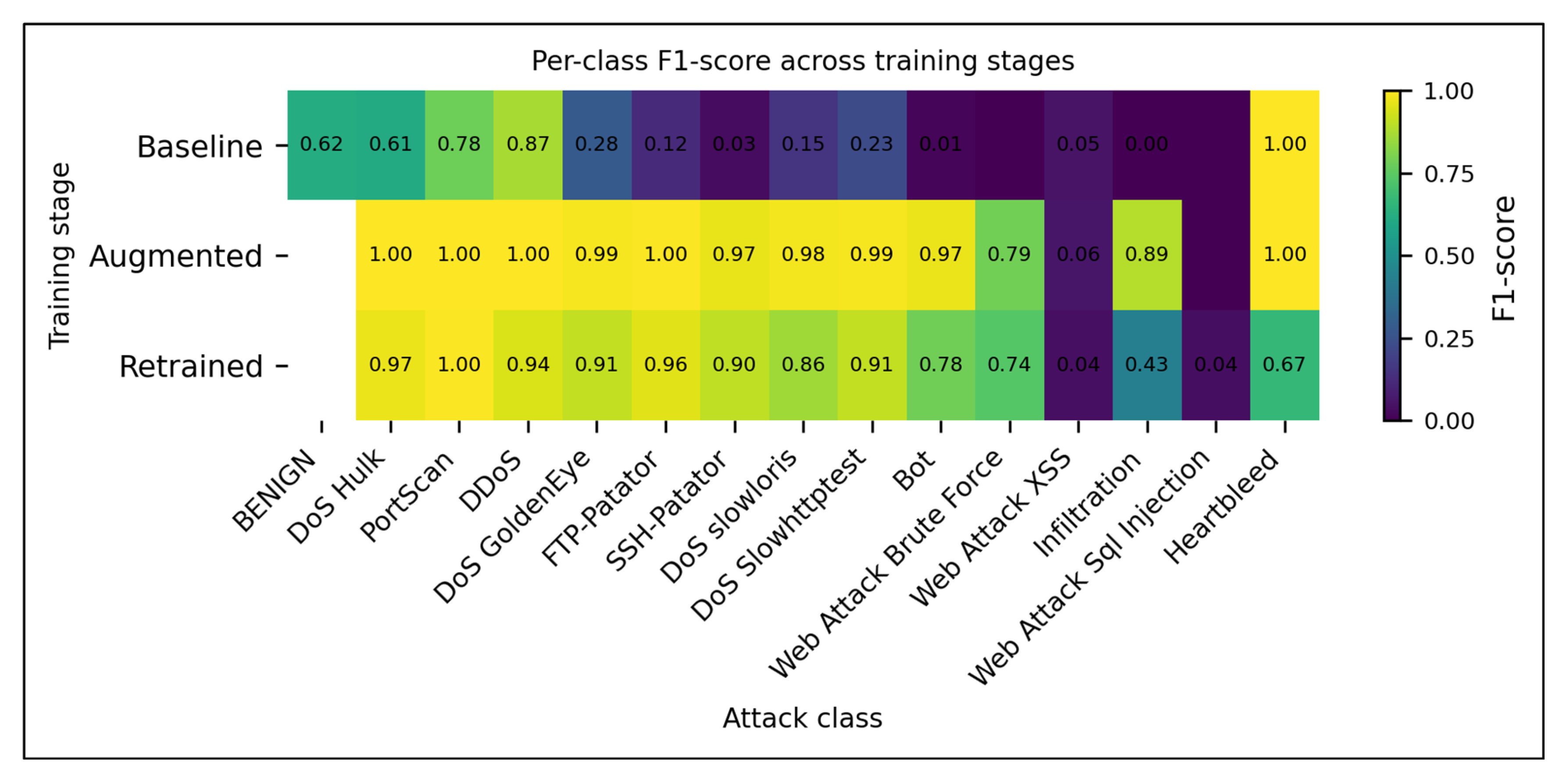
Per-class F1-scores for CNN–LSTM across the three pipeline stages (baseline, GAN-augmented, and feedback-retrained). Augmentation boosts F1 dramatically for most minority classes (e.g., FTP-Patator, SSH-Patator, Bot), and uncertainty-guided retraining preserves most of those gains while stabilizing benign performance. The values embedded in each cell represent the exact classwise F1.
Figure 13.
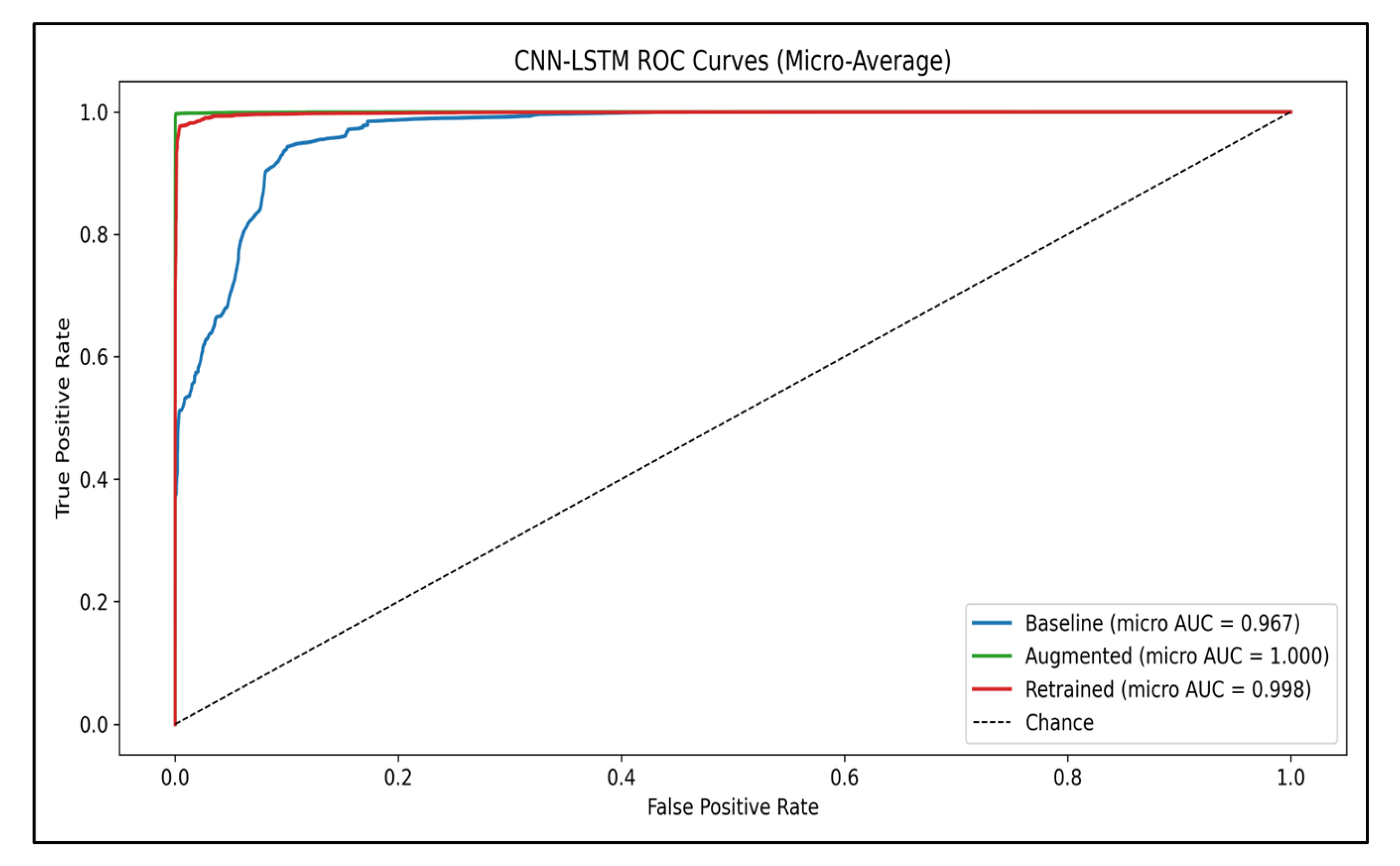
Micro-averaged ROC curves for CNN–LSTM across the three stages (baseline, augmented, and retrained). Augmentation lifts the curve to almost perfect separability (AUC = 1.000), and uncertainty-guided retraining retains that performance (AUC = 0.998), whereas the baseline remains high at AUC = 0.967. The dashed line indicates a chance classifier.
Figure 14.
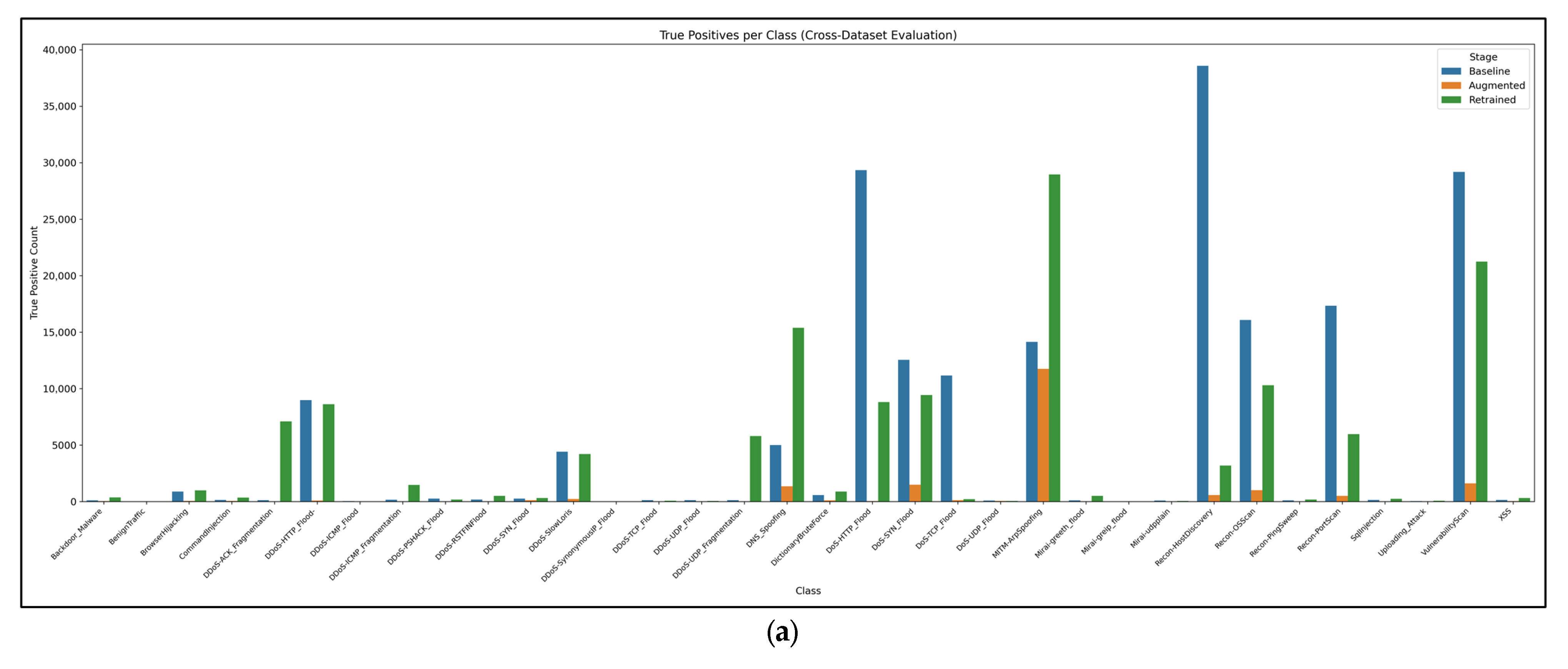
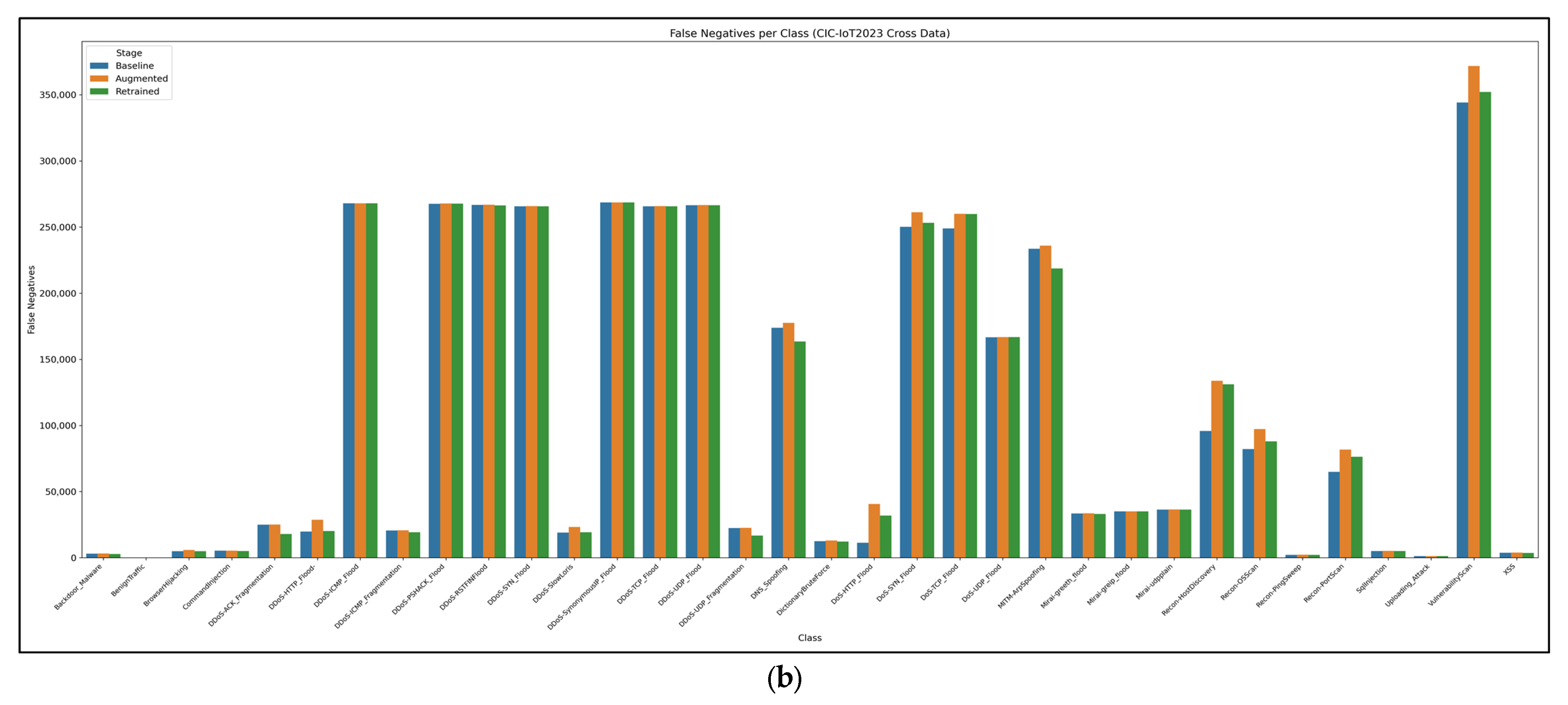
(a) True-positive counts per IoT attack class for the baseline, augmented, and retrained CNN–LSTM stages. (b) Corresponding false-negative counts. Cross-dataset transfer is dominated by a few Mirai/DDoS classes, whereas most IoT-specific malware remains largely undetected, underscoring a severe domain shift.
Figure 15.
Reliability diagrams for the CNN–LSTM binary classifier at each pipeline stage. The baseline (left) remains close to the diagonal (ECE ≈ 0.04, Brier ≈ 0.11); augmentation (middle) is strongly overconfident, with bins diverging from the diagonal (ECE ≈ 0.62, Brier ≈ 0.51); and retraining (right) partially realigns the probabilities (ECE ≈ 0.32, Brier ≈ 0.28).
Table 1.
Comparison of the IDS studies mentioned above.
Table 1.
Comparison of the IDS studies mentioned above.
| Study (Year) | Dataset(s) Used | IDS Model Type | Imbalance Strategy | Cross-Dataset Eval? | Calibration? | Human-in-Loop? |
|---|
| Shahriar et al. (2024) [26] | V2X network traces (simulated vehicular attacks) | GAN-based (ensemble WGAN, “VEHIGAN”) | Generative oversampling | No | No | No |
| Strickland et al. (2023) [27] | NSL-KDD | Hybrid GAN + DRL (DRL-GAN framework) | GAN minority oversampling | No | No | No |
| Kim et al. (2024) [30] | Simulated alert stream (based on IDS data) | Active learning framework (model-agnostic) | None (active query strategy) | No | No | Yes (analyst feedback loop) |
| Alohali et al. (2025) [32] | IoHT network traces (healthcare IoT) | Ensemble (multiple classifiers) | None (focus on ensemble learning) | No | Yes (Temperature scaling applied) | No |
| Hussain et al. (2025) [35] | UNSW-NB15; CIC-DDoS2019; Kitsune (WSN/IoT) | Ensemble (DRL + LSTM in “MultiNet-IDS”) | None (feature selection used for efficiency) | No | No | No |
| Hossain (2025) [36] | CIC-IoT2023 (IoT traffic) | CNN, LSTM, RNN, MLP (1D CNN found best) | None (standard training) | No | No | No |
| Manocchio et al. (2023) [37] | CIC-IDS2017; NSL-KDD; UNSW-NB15 | Transformer-based (Flow Transformer) | None (pre-training for feature learning) | No | No | No |
| He et al. (2024) [38] | CIC-IDS2017; NSL-KDD; UNSW-NB15 | Transformer-based (Vision Transformer) | None (image-based feature encoding) | No | No | No |
| Sinha et al. (2025) [39] | NSL-KDD; CIC-IDS2017; UNSW-NB15; CTU-13 (WSN) | CNN + adversarial training (WSN-IDS) | SMOTE oversampling used | Yes (evaluated transfer across sets) | No | No |
| Ebrahimi et al. (2025) [40] | TON_IoT (IoT telemetry) | CNN classifier (+ explainable AI) | None (focus on feature selection) | No | No | No |
| Haque (2020) [41] | NSL-KDD (subset for low-sample demo) | Semi-supervised (EC-GAN + classifier) | GAN data augmentation | No | No | No |
| Our Approach (2025) | CIC-IDS2017 (primary), CIC-IoT2023 (cross-eval) | Calibrated CNN–LSTM | VAE-seeded cWGAN-GP generative balancing | Yes (CIC-IDS2017 → CIC-IoT2023) | Yes (temperature scaling; ECE/Brier reported) | Yes (uncertainty-based analyst deferral) |
Table 2.
The main hardware environment of the experiment.
Table 2.
The main hardware environment of the experiment.
| Component | Description | Quantity |
|---|
| CPU | Intel i7-12700H | 1 |
| Graphics | Nvidia GeForce RTX 3050 Ti 32G | 1 |
| Memory | 32 GB | 1 |
| Programing Language | Python 3.11 | - |
Table 3.
CIC-IDS2017 class distribution.
Table 3.
CIC-IDS2017 class distribution.
| Class ID | Class | Count | Proportion (%) | Imbalance Ratio | Train | Val | Test |
|---|
| 0 | BENIGN | 2,273,097 | 80.3004 | 1.0000 | 1,591,167 | 340,964 | 340,966 |
| 1 | DoS Hulk | 231,073 | 8.1630 | 9.8371 | 161,751 | 34,660 | 34,662 |
| 2 | Port Scan | 158,930 | 5.6144 | 14.3025 | 111,251 | 23,839 | 23,840 |
| 3 | DDoS | 128,027 | 4.5227 | 17.7548 | 89,618 | 19,204 | 19,205 |
| 4 | DoS GoldenEye | 10,293 | 0.3636 | 220.8391 | 7205 | 1543 | 1545 |
| 5 | FTP-Patator | 7938 | 0.2804 | 286.3564 | 5556 | 1190 | 1192 |
| 6 | SSH-Patator | 5897 | 0.2083 | 385.4667 | 4127 | 884 | 886 |
| 7 | DoS Slowloris | 5796 | 0.2048 | 392.1837 | 4057 | 869 | 870 |
| 8 | DoS Slowhttptest | 5499 | 0.1943 | 413.3655 | 3849 | 824 | 826 |
| 9 | Bot | 1966 | 0.0695 | 1156.2040 | 1376 | 294 | 296 |
| 10 | Web Attack Brute Force | 1507 | 0.0532 | 1508.3599 | 1054 | 226 | 227 |
| 11 | Web Attack XSS | 652 | 0.0230 | 3486.3451 | 456 | 97 | 99 |
| 12 | Infiltration | 36 | 0.0013 | 63,141.5833 | 25 | 5 | 6 |
| 13 | Web Attack Sql Injection | 21 | 0.0007 | 108,242.7143 | 14 | 3 | 4 |
| 14 | Heartbleed | 11 | 0.0004 | 206,645.1818 | 7 | 1 | 3 |
Table 4.
Synthetic sample counts per class (cWGAN-GP augmentation plan).
Table 4.
Synthetic sample counts per class (cWGAN-GP augmentation plan).
| Class Id | Class | Current Count | Reason | Synthetic to Generate | Final Count |
|---|
| 1 | DoS Hulk | 231,073 | none | 0 | 231,073 |
| 2 | Port Scan | 158,930 | none | 0 | 158,930 |
| 3 | DDoS | 128,027 | none | 0 | 128,027 |
| 4 | DoS GoldenEye | 10,293 | none | 0 | 10,293 |
| 5 | FTP-Patator | 7938 | none | 0 | 7938 |
| 6 | SSH-Patator | 5897 | none | 0 | 5897 |
| 7 | DoS Slowloris | 5796 | none | 0 | 5796 |
| 8 | DoS Slowhttptest | 5499 | none | 0 | 5499 |
| 9 | Bot | 1966 | minority | 7864 | 9830 |
| 10 | Web Attack Brute Force | 1507 | minority | 6028 | 7535 |
| 11 | Web Attack XSS | 652 | minority | 4348 | 5000 |
| 12 | Infiltration | 36 | minority | 4964 | 5000 |
| 13 | Web Attack Sql Injection | 21 | minority | 4979 | 5000 |
| 14 | Heartbleed | 11 | minority | 4989 | 5000 |
Table 5.
CNN–LSTM Classifier Architecture and Training Hyperparameters.
Table 5.
CNN–LSTM Classifier Architecture and Training Hyperparameters.
| Component | Configuration |
|---|
| Input Shape | (D *, 1), where D = number of features (original D = 79, after tuned D = 46) |
| Conv1D Layer 1 | 64 filters, kernel size = 5, activation = ReLU |
| MaxPooling1D | Pool size = 2 |
| Conv1D Layer 2 | 128 filters, kernel size = 3, activation = ReLU |
| LSTM Layer | 128 units, return sequences = False |
| Dropout | 0.30 |
| Output Layer *** | Dense, Softmax activation, C ** classes |
| Optimizer | Adam |
| Learning Rate | |
| Loss Function | Sparse Categorical Cross-Entropy |
| Batch Size | 256 |
| Metrics | Accuracy |
Table 6.
Multi-class baseline results. Macro/weighted metrics across all classes and micrometrics across attack classes only. Support counts reflect the number of flows per split. Weighted averages are dominated by the Benign class; therefore, macro-attack metrics provide a better picture of rare-attack detection.
| Class | Precision | Recall | F1-Score | Support |
|---|
| BENIGN | 0.9999804604813235 | 0.4502880069450147 | 0.6209597997164807 | 340,964.0 |
| DoS Hulk | 0.4455149934810952 | 0.9858630737716743 | 0.613697793662054 | 34,661.0 |
| PortScan | 0.6380619111709287 | 0.9943370107806535 | 0.7773205004181082 | 23,839.0 |
| DDoS | 0.806774787726313 | 0.9351176838158717 | 0.8662180739454454 | 19,204.0 |
| DoS GoldenEye | 0.17060753478900328 | 0.9766839378238342 | 0.2904748146007898 | 1544.0 |
| FTP-Patator | 0.06636155606407322 | 0.9991596638655462 | 0.12445700528602083 | 1190.0 |
| SSH-Patator | 0.016444660630098033 | 0.994343891402715 | 0.03235424028268551 | 884.0 |
| DoS slowloris | 0.08421052631578947 | 0.7908045977011494 | 0.15221238938053097 | 870.0 |
| DoS Slowhttptest | 0.1303397241843256 | 0.9393939393939394 | 0.22891744203219613 | 825.0 |
| Bot | 0.006385368201508102 | 0.6745762711864407 | 0.012650985378258105 | 295.0 |
| Web Attack Brute Force | 0.0 | 0.0 | 0.0 | 226.0 |
| Web Attack XSS | 0.02601578485822859 | 0.9081632653061225 | 0.05058255186132424 | 98.0 |
| Infiltration | 0.0014819205690574985 | 0.8333333333333334 | 0.0029585798816568047 | 6.0 |
| Web Attack Sql Injection | 0.0 | 0.0 | 0.0 | 3.0 |
| Heartbleed | 0.6666666666666666 | 1.0 | 0.8 | 2.0 |
| accuracy | 0.5527388598034436 | 0.5527388598034436 | 0.5527388598034436 | 0.55273 |
| macro avg | 0.27058972634256073 | 0.7654709783550864 | 0.30485361176303666 | 424,611.0 |
| weighted avg | 0.9129459389692415 | 0.5527388598034436 | 0.633800109576285 | 424,611.0 |
Table 7.
Quantitative evaluation of synthetic sample quality across selected attack classes using FID, MMD, and JSD. Lower values across all three metrics indicate a higher similarity between the real and synthetic distributions. These metrics were computed over 46-dimensional network flow features.
| Class ID | FID | MMD | JSD | Num. Real | Num. Synthetic |
|---|
| 9 | 5.616491010801062 | 0.5094026923179626 | 0.688205360212883 | 1966 | 7864 |
| 10 | 5.273963760298355 | 0.7643402218818663 | 0.6900884240235304 | 1507 | 6028 |
| 11 | 5.261420908135975 | 0.981743395328501 | 0.6887034792844112 | 652 | 4348 |
| 12 | 4.738063261646395 | 0.2298018932322524 | 0.6558891723687298 | 36 | 4964 |
| 13 | 5.509566043010276 | 0.6236924529074456 | 0.6918680648782362 | 21 | 4979 |
| 14 | 5.241619543532286 | 0.6988047361373197 | 0.6816343053751411 | 11 | 4989 |
Table 8.
Calibration of CNN–LSTM across training stages.
Table 8.
Calibration of CNN–LSTM across training stages.
| Stage | Decision Threshold | Expected Calibration Error | Brier Score | Description |
|---|
| Baseline | 0.20 | 0.041 | 0.109 | Baseline posteriors are well behaved: the reliability diagram follows the diagonal, indicating that the model's probabilities align with the observed event frequencies. |
| Augmented | 1.00 | 0.618 | 0.513 | GAN-based oversampling and the aggressive threshold push benign precision toward zero, creating large calibration errors. The reliability diagram shows bins far from the diagonal. |
| Retrained | 0.80 | 0.323 | 0.284 | Feedback-driven retraining partially restores calibration: both ECE and Brier fall between the baseline and augmented scores. The reliability diagram shows partial realignment toward the diagonal, though benign probabilities remain over-confident. |
Table 9.
Cross-dataset evaluation on CIC-IoT2023.
Table 9.
Cross-dataset evaluation on CIC-IoT2023.
| Stage | Threshold | Samples | Accuracy (%) | Recall |
|---|
| Baseline | 0.90 | 4,343,217 | 20.04 | 23.09 |
| Augmented | 1.00 | 4,343,217 | 9.98 | 3.23 |
| Retrained | 1.0 | 4,343,217 | 59.83 | 59.88 |
Table 10.
Adversarial Robustness of the Retrained Model.
Table 10.
Adversarial Robustness of the Retrained Model.
| Attack | Epsilon | Accuracy |
|---|
| Clean | - | 0.656 |
| FGSM | 0.005 | 0.537 |
| PGD | 0.01 | 0.409 |
Table 11.
Macro-averaged precision, recall, and F1-score across the stages.
Table 11.
Macro-averaged precision, recall, and F1-score across the stages.
| Stage | Macro Precision | Macro Recall | Macro F1-Score |
|---|
| Baseline | 0.271 | 0.765 | 0.305 |
| Augmented | 0.920 | 0.979 | 0.927 |
| Retrained | 0.789 | 0.865 | 0.779 |
Table 12.
Performance comparison of different intrusion detection methods on the CIC-IDS2017 dataset.
Table 12.
Performance comparison of different intrusion detection methods on the CIC-IDS2017 dataset.
| Model | Accuracy | Precision | Recall | F1-Score |
|---|
| KNN-TACGAN [44] | 95.86% | 96.85% | 94.79% | 95.81% |
| KD-TCNN [45] | 99.44% | 99.48% | 99.47% | 99.46% |
| GAN-RF [46] | 99.83% | 98.68% | 92.76% | 95.04% |
| RTIDS [47] | 99.35% | 98.89% | 98.83% | 99.17% |
| Transformers [48] | 93.135 | 99.22% | 99.13% | 99.16% |
| Ours * (Calibrated CNN-LSTM) | 98.03% | 92.10% | 96.55% | 94.30% |
