Article

Addressing Uncertainty by Designing an Intelligent Fuzzy System to Help Decision Support Systems for Winter Road Maintenance

by
Mahshid Hatamzad
1,*,
Geanette Polanco Pinerez
1 and
Johan Casselgren
2
1
Department of Industrial Engineering, UiT/The Arctic University of Norway, 8514 Narvik, Nordland, Norway
2
Department of Engineering Sciences and Mathematics, Luleå University of Technology, 971 87 Luleå, Sweden
*
Author to whom correspondence should be addressed.
Safety 2022, 8(1), 14; https://doi.org/10.3390/safety8010014
Submission received: 1 November 2021 / Revised: 26 January 2022 / Accepted: 15 February 2022 / Published: 17 February 2022

Abstract

:
One of the main challenges in developing efficient and effective winter road maintenance is to design an accurate prediction model for the road surface friction coefficient. A reliable and accurate prediction model of road surface friction coefficient can help decision support systems to significantly increase traffic safety, while saving time and cost. High dynamicity in weather and road surface conditions can lead to the presence of uncertainties in historical data extracted by sensors. To overcome this issue, this study uses an adaptive neuro-fuzzy inference system that can appropriately address uncertainty using fuzzy logic neural networks. To investigate the ability of the proposed model to predict the road surface friction coefficient, real data were measured at equal time intervals using optical sensors and road-mounted sensors. Then, the most critical features were selected based on the Pearson correlation coefficient, and the dataset was split into two independent training and test datasets. Next, the input variables were fuzzified by generating a fuzzy inference system using the fuzzy c-means clustering method. After training the model, a testing set was used to validate the trained model. The model was evaluated by means of graphical and numerical metrics. The results show that the constructed adaptive neuro-fuzzy model has an excellent ability to learn and accurately predict the road surface friction coefficient.

1. Introduction

1.1. Motivation

Low temperatures and heavy snowfall can be problematic for road users, especially in countries with long and harsh cold-weather conditions. Road safety can be significantly reduced due to slippery surface conditions and poor visibility [1]. Adverse weather can decrease the reliability and productivity of the surface transportation system. In addition, it increases traffic delays and the likelihood of vehicle accidents that may lead to severe injuries and fatalities [2]. To minimize these negative impacts, roads must be kept clear of ice and snow through chemical (salting) and mechanical (plowing) operations, referred to as winter road maintenance (WRM) techniques. WRM helps to increase the friction between tires and the road surface to prepare the road for normal traffic flow, meaning that the road users can drive as fast as in summer (effective WRM); however, this can result in high expenses (inefficient WRM).
Prediction of the road surface friction coefficient (RSFC) can help decision makers to plan in advance for the type and timing of WRM to improve decision support systems (DSS). The prediction of RSFC is a comprehensive calculation from different performance aspects using multiple physical dynamic variables (e.g., weather temperature, ice layer, snow height, etc.), which often shows a nonlinear relationship between road surface friction and the considered variables. In fact, sensors are not always able to measure road surface conditions (RSC) precisely, due to various reasons such as signal noise. Therefore, uncertainties need to be considered to enhance the accuracy of prediction models and improve the WRM performance.

1.2. Significance of the Topic

An accurate RSFC prediction model helps decision makers to effectively prepare for and respond to severe road conditions in winter (such as snowstorms and sharp reductions in RSFC), in order to maximize road safety for road users. Addressing uncertainty in a prediction model allows decision makers to systematically prevent hazards (such as fatal vehicle accidents) and strategically organize WRM resources to mitigate the detrimental impacts that a disaster can cause. In addition, avoiding the use of extra salt (chemicals) on the road surface minimizes cost and environmental impacts. In fact, high WRM quality and using an optimal salt quantity minimizes damage to vehicles, road infrastructure, vegetation, lakes, rivers, etc.

1.3. State-of-the-Art Method

There are several studies that present various methods to reach effective and efficient WRM. Shao and Lister [3], the authors used air temperature, wind speed, surface temperature, and dew-point as input variables to develop an automated road ice prediction model. Mohseni [4] applied a regression model to select the strongest features (pavement temperature, latitude, air temperature, elevation, and depth into the asphalt concrete layer) to develop a prediction model for low pavement temperature based on laboratory tests. Kangas et al. [5] developed a simulation model named RoadSurf using numerical weather forecasts as input to predict road surface temperature and condition. Moreover, developing sensor technologies has had a significant impact on monitoring road surface conditions in winter. Ye et al. [6] presented a review about developing and implementing advanced technologies to achieve safe and efficient WRM. Ewan et al. [7] investigated the reliability of an optical sensor to measure snow depth, water depth, and surface state (dry, wet, icy, etc.). Feng and Fu [8] investigated the performance of pavement sensors, and their results show that a sensor cannot always detect friction precisely. However, WRM effectiveness and efficiency can be improved by developing data-driven approaches using historical data collected by sensors. Ahabchane et al. [9] proposed a data-driven regression model using geometry, weather, and telemetry data to predict the amount of salt and abrasives in street segments. Pan et al. [10] applied deep neural networks to classify RSC according to images. Liu et al. [11] utilized machine learning algorithms (gradient-boosting) to develop road surface temperature forecasting. Roychowdhury et al. [12] applied neural networks to design a methodology to estimate RFSC. Panahandeh et al. [13] employed machine learning (ML) classification algorithms to predict RFCS for connected vehicles. Pu et al. [14] developed a daily RSFC prediction model using a long–short-term memory neural network based on the following three scenarios: (i) considering only daily friction data, (ii) selecting water thickness as an input variable, and (iii) selecting road surface temperature and water thickness as predictors. Their results showed that the second scenario had the highest accuracy. ML algorithms are powerful techniques to predict different nonlinear problems. Optical and road-mounted sensors are mostly used to measure data-related road surface conditions. Sometimes, numerical data derived from sensors can be associated with uncertainty due to imprecision, vagueness, or ambiguity. Song et al. [15] estimated maximum RSFC under uncertainty using deep learning. Matusko et al. [16] presented a new approach by adding neural networks to the friction estimator model, to enhance the estimation quality by compensating for the impacts of uncertainties. Kim et al. [17] designed a system for composite friction control, which included friction uncertainty using recurrent fuzzy neural networks. While previous research studies have contributed significantly to developing different dimensions of WRM, there has, thus far, been no study to predict RSFC by designing an adaptive neuro-fuzzy inference system (ANFIS), which is able to handle the uncertainty hidden in historical data extracted by sensors. An adaptive fuzzy RSFC prediction model with high accuracy plays an important role in making WRM plans in advance, in order to achieve effective and efficient WRM.

1.4. Contributions

Reviewing previous studies on WRM reveals that it is not easy to establish an accurate data-driven RSFC prediction model, due to dynamic weather conditions that can lead to variation in road surface conditions. In addition, historical data collected by sensors can be associated with uncertainty, which must be modeled. To model this complex problem, the main contribution of this study is the design of an ANFIS model to predict RSFC using real data measured by optical and road-mounted sensors. The ANFIS model fuzzifies the crisp data for simulating this complex problem, associated with uncertainty.

1.5. Outline of the Paper

The remainder of this paper is organized as follows. Section 2 explains the summary of ANFIS. The data and methods are defined in Section 3. In Section 4, we present results. Finally, in Section 5, a conclusion is drawn.

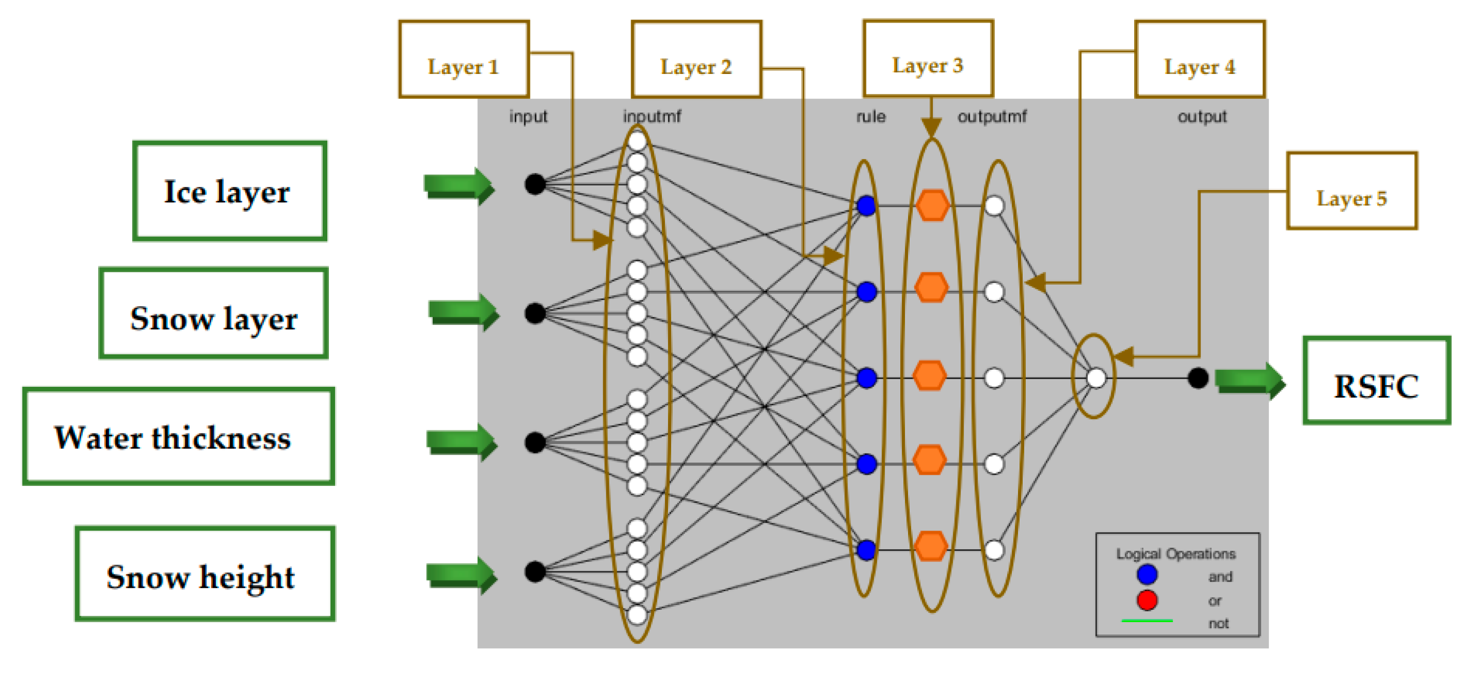
2. Adaptive Neuro-Fuzzy Inference System (ANFIS)
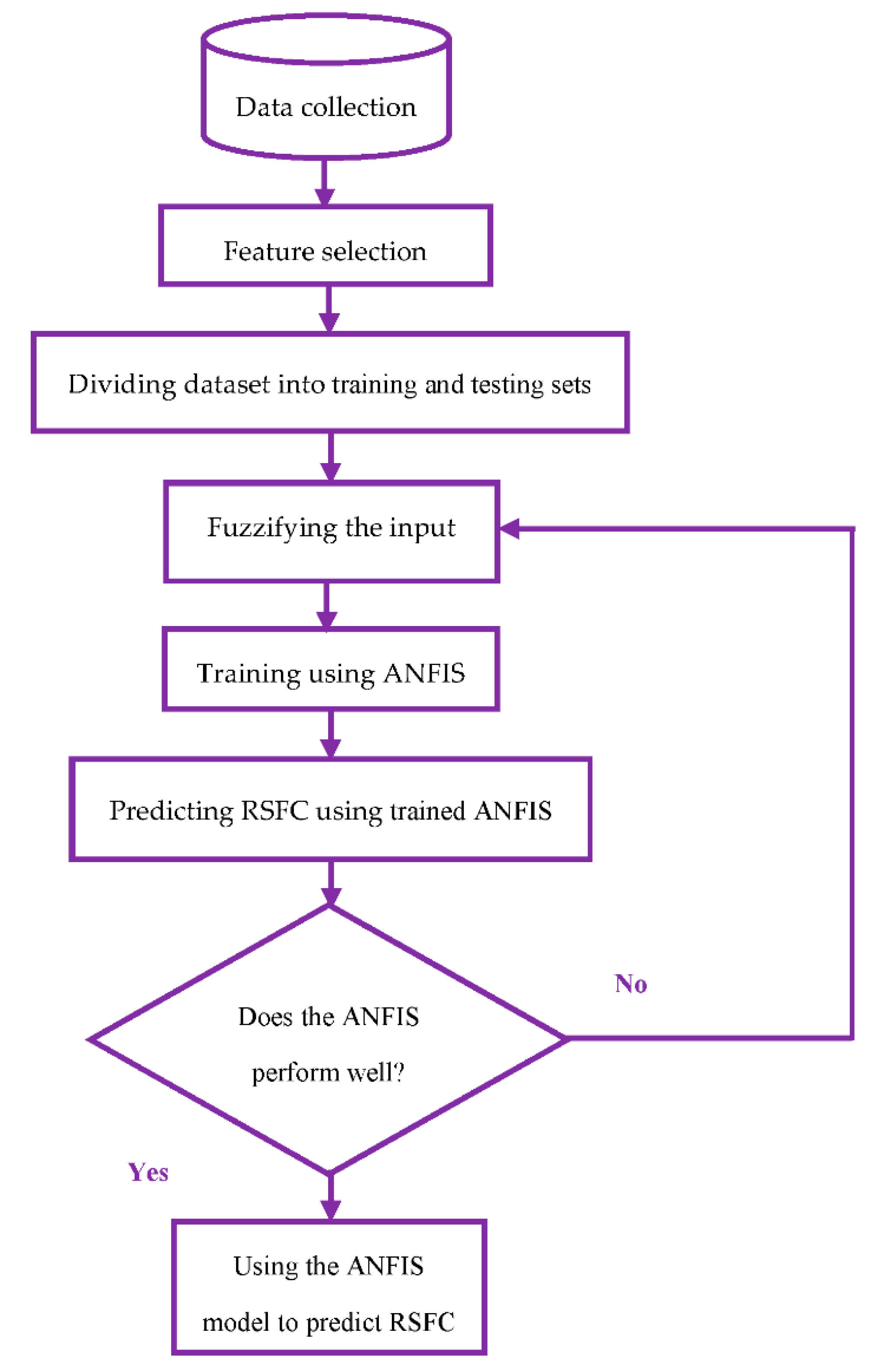
Crisp numerical data points can be fuzzified and represented by membership functions (MFs) [18]. In recent years, artificial intelligence methods, including fuzzy intelligent techniques, have been extensively used in different fields such as economics, medicine, and engineering. The ANFIS model was proposed by Jang in the 1990s [19] and can be considered as a universal estimator for predicting long- and short-term effects [20]. ANFIS is a five-layer adaptive network that illustrates the relationship between inputs and outputs to simulate complex problems associated with uncertainties by creating fuzzy variables [21]. The ANFIS network utilizes the learning ability of neural network concepts and the reasoning mechanisms of the Takagi–Sugeno fuzzy interference system (FIS) [22]. Due to using both fuzzy logic and neural networks, ANFIS can benefit from both models’ principles in a single model. The inference system employs fuzzy “if-then” rules, which have a learning ability to estimate nonlinear functions [23].

3. Data and Methods

Figure 1 shows the framework of this study and its different steps, which are explained in this section.

3.1. Data Collection

Although there is an obvious relationship between road surface conditions and weather conditions, the proposed model’s input variables are defined as conditions that impact the WRM performance. In addition, the output variable is defined as a result gained from the input variables. One of the major benefits of the data-driven model is that different kinds of inputs and outputs are allowed to be included in the model without having special relationships. Moreover, all of the input variables have a similar opportunity to affect the road conditions. Therefore, here, air temperature, surface temperature, ice layer, snow layer, water thickness, and snow height were chosen as input variables and RSFC was chosen as the output variable. Historical data of these variables were measured every 10 min and collected from the Swedish Transport Administration’s RWIS station on a European road at test site E18 in February 2019. The test site E18 is located in Sweden, Northern Europe, between Enköping and Västerås, the latitude and longitude are approximately 59.724 and17.029 [24], and the type of pavement was asphalt. The road weather station measured air temperature. Optical sensors measured ice layer (mm), snow layer (mm) (new snow), and RSFC. A road-mounted sensor measured surface temperature (°C), snow height (mm) (both new and old snow), and water thickness (mm). Table 1 shows the statistical description of the dataset.
In Table 1, the first column shows the number of observations, which are equal for all variables. The second and third columns illustrate the mean value and standard deviation of observations, respectively. The fourth and eighth columns are the minimum and maximum values for each variable. The fifth, sixth, and seventh columns demonstrate the 25th percentile (the lower or first quartile), 50th percentile (the median), and 75th percentile (the upper or third quartile), respectively.

3.2. Feature Selection

In the previous step, variables influencing RSFC were initially chosen. However, reducing the number of input variables decreases the model complexity and enhances the training process, which can lead to enhancing the model accuracy. Therefore, we used the Pearson correlation coefficient to select the most significant predictors. Table 2 shows the absolute value of correlation between the input variables and RSFC. Out of six input variables, four variables (ice layer, snow layer, water thickness, and snow height) were highly correlated with RSFC. Thus, these four input variables were used to design an RSFC prediction model.

3.3. Dividing the Dataset into Training and Testing Sets

The dataset needed to be divided into training and testing sets. The training dataset optimizes the parameters of the model, and the test dataset evaluates the model performance to predict RSFC. In this study, 70% of the observations were considered for training the ANFIS model and the rest of the observations were applied to test the model, since the testing set needs to be large enough to lead to meaningful statistical results. Table 3 shows the statistical information of the testing set.

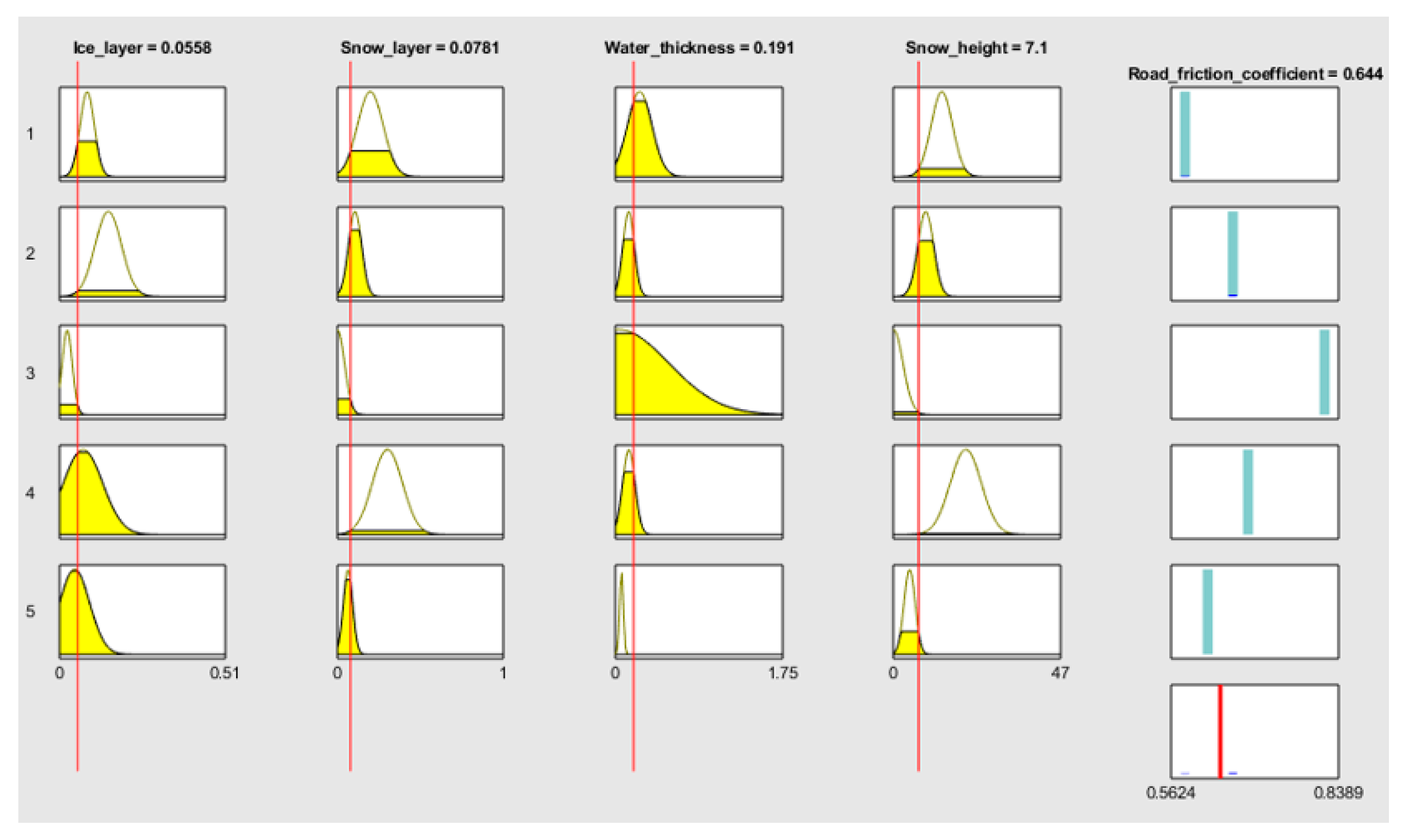
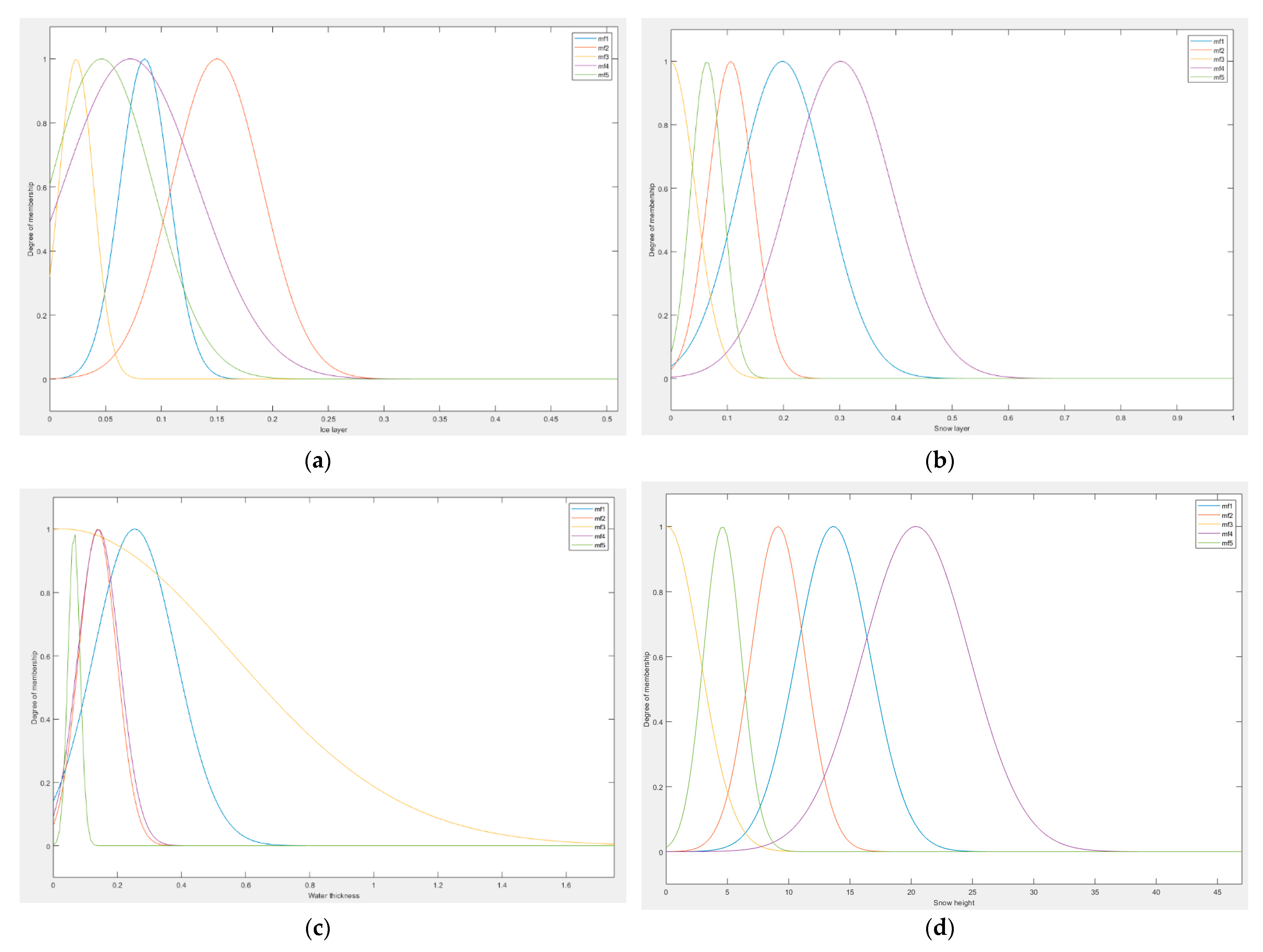
3.4. Generating Basic Fuzzy Inference System

In this stage, input variables were fuzzified by using Genfis3 in Matlab software. Genfis3 generates a structure based on the fuzzy inference system (FIS) using the fuzzy c-means (FCM) clustering method by extracting some fuzzy rules, which model the data behavior. The number of clusters specifies the number of rules and membership functions. We selected the ‘Sugeno’ type because Sugeno is more flexible to design a system more precisely [20]. The number of clusters was five, and the clustering (FCM) options were selected according to the default values in Matlab. The types of the input and output MFs were Gaussian and Linear, respectively. The number of input and output MFs (clusters) was five, equal to the number of fuzzy rules.

3.5. Training Using ANFIS

The training epoch number was set as 200, the initial step size was 0.01 with a decrease rate of 0.9 and an increase rate of 1.1, and the hybrid method was selected as the optimization method [25]. Increasing and decreasing the step sizes balances the exploration and exploitation to enhance the convergence speed and drive the process from the local minimum solution.

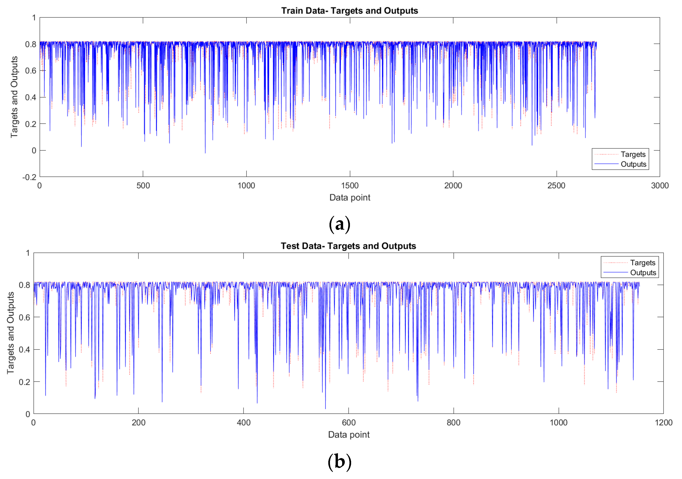
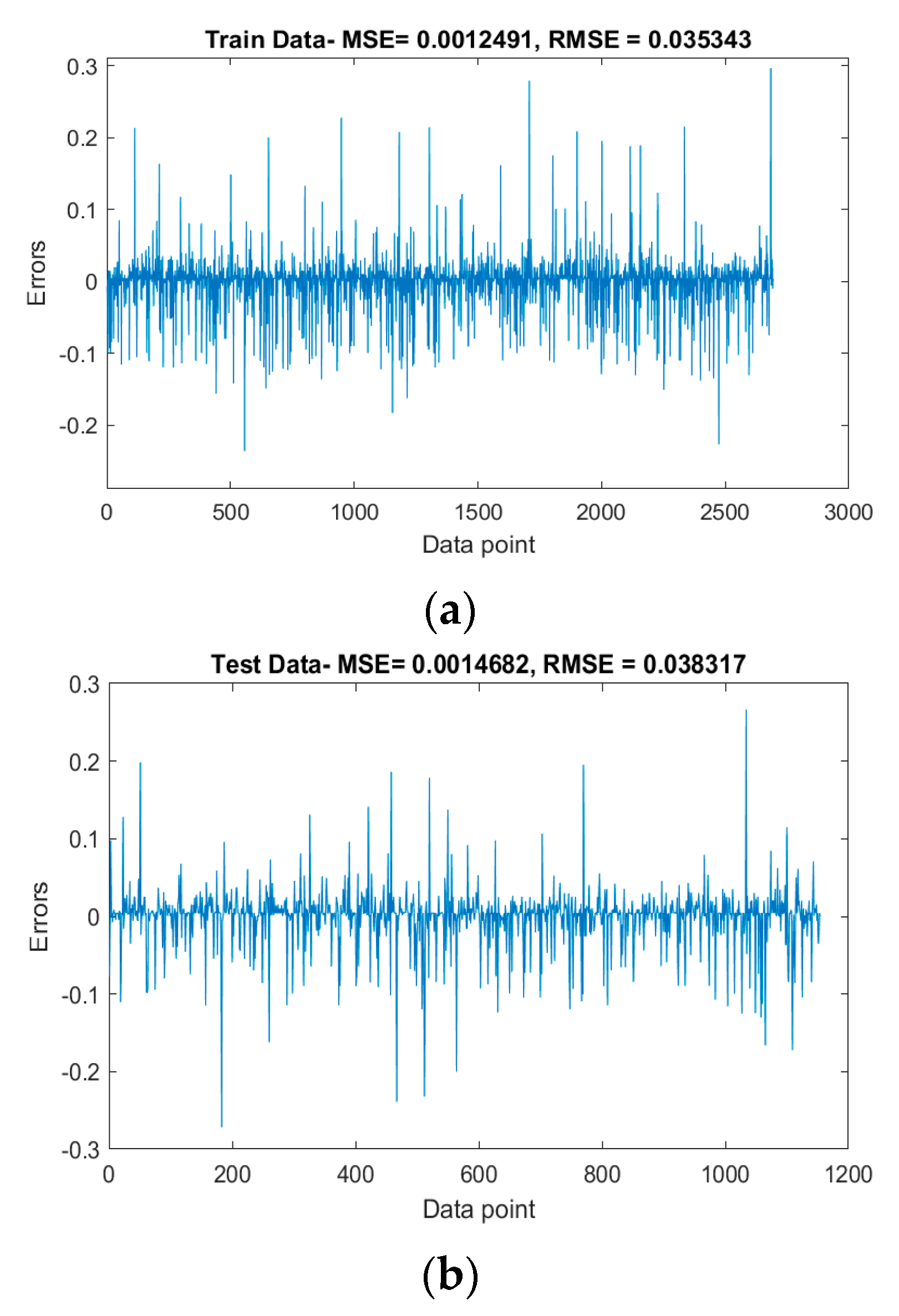
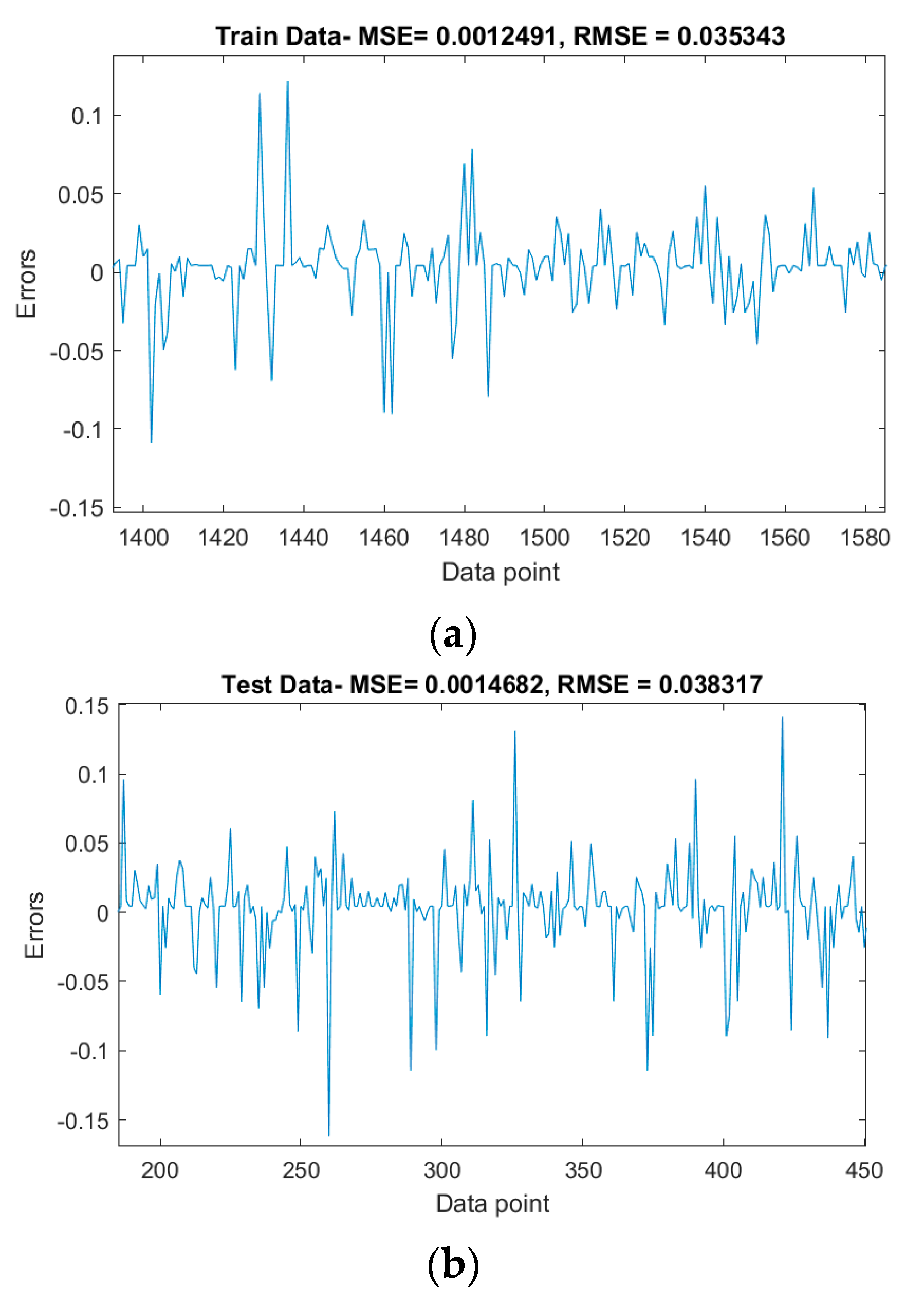
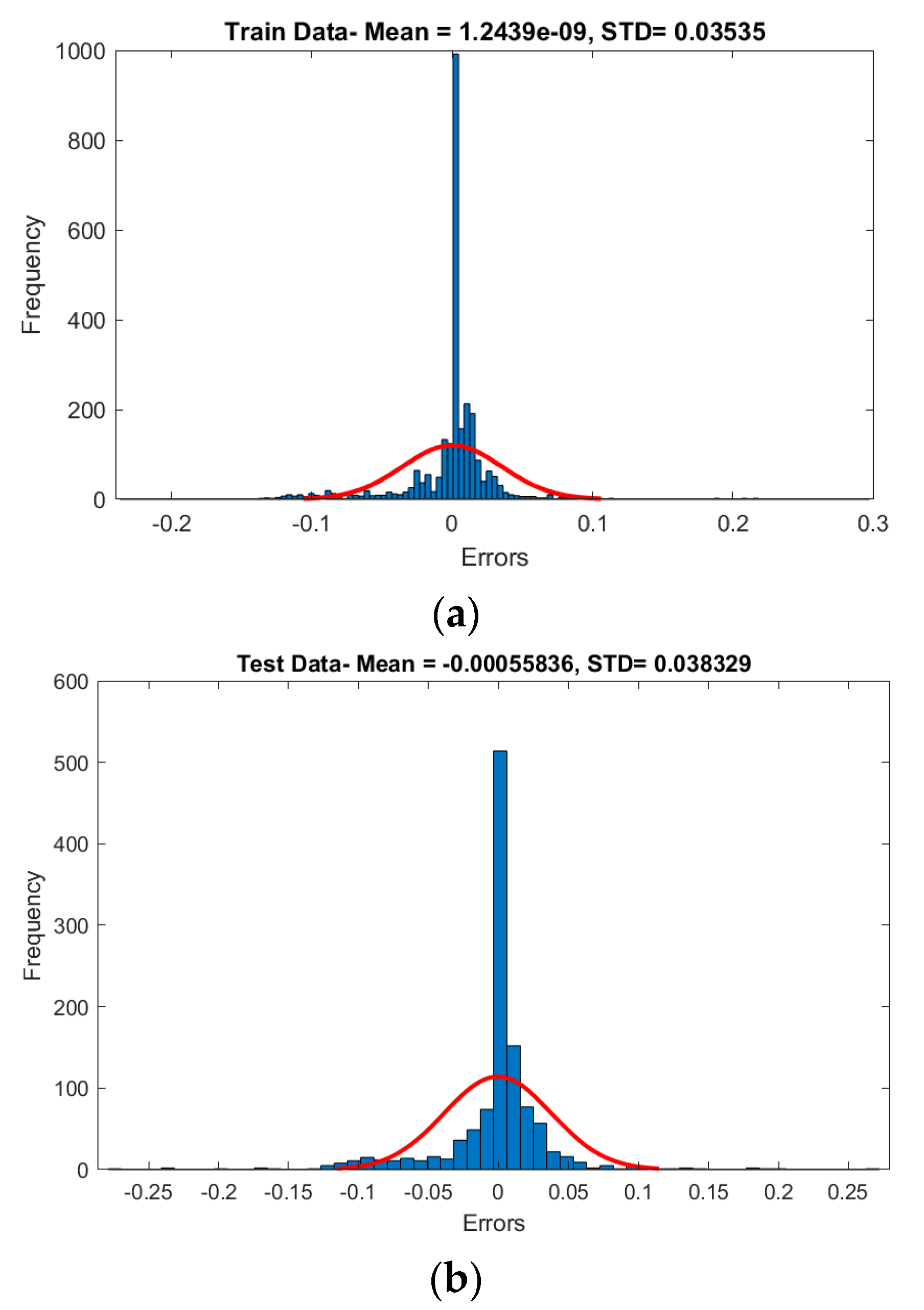
3.6. Evaluating Performance of ANFIS

A total of 3847 data points were considered in this study, of which 2693 (70%) observations were for training and 1154 (30%) were for testing the model. Figure 2 and Table 4 depict the structure of the ANFIS network designed in this study to predict the RSFC in winter. In fact, five layers built the ANFIS model based on node functions. The first layer was the “if part”, or fuzzification; the second layer was implications (rules); the third layer was normalization; the fourth layer was the “then part”, or defuzzification; and the fifth layer was the summation part (output) [20]. According to the collected road dataset, the fuzzy clustering of the predictors for a one-month period is presented in Figure 3. The degree of membership was between 0 and 1. A degree of membership of 0 means that the value does not belong to the given fuzzy set. A degree of membership of 1 means the value certainly belongs to the given fuzzy set. However, if the value of membership is between 0 and 1, it demonstrates the degree of uncertainty with which the value belongs in the given fuzzy set. The information and parameters of the MFs for each input (i.e., mean and standard deviation) and output (coefficients and constant) are shown in Table 5, Table 6 and Table 7. We considered five clusters for each input, and the output based on trial and error, which demonstrated the best results.
After building the base FIS, the model was trained by ANFIS. Figure 4 shows a 3D view of the relationship between the ice layer, snow layer, and RSFC. A 3D view of the relationship between parameters helps us to extract the relationship between effective variables to predict RSFC. For instance, in Figure 4, if the value of the ice layer is less than 0.3, the value of the snow layer has no measurable impact on the created value of the RSFC. The ANFIS rule viewer (for trained data) is shown in Figure 5. Each input column displays five Gaussian membership functions for each input variable and each row shows a particular rule. Hence, each membership function has a specific rule and maps the values of each input variable to rule input values. The output column indicates how various rules can be applied to the RSFC (output variable) [26].
Figure 6, Figure 7, Figure 8, Figure 9 and Figure 10 visualize ANFIS performance for the training and test datasets. The graphs demonstrate that predicted values are close to the real values most of the time. Only a few numbers show obvious errors, which could be due to (i) these targets not being scientifically justifiable, or (ii) this method not being suitable to predict these targets. Figure 10 shows the residual plots that show the difference between real values and predicted values for both the training and testing datasets. As is clear, the value of 0 in the residual plots has the highest number and the residual plots are normally distributed, which means that ANFIS is the correct selection for our dataset. In addition, MSE and RMSE were selected as the evaluation metrics to evaluate the model performance (Table 8). RMSE values for the training and test datasets are 0.035 and 0.038, respectively. The low error of the test set indicates that the ANFIS model has a good generalization performance to effectively predict RSFC based on historical data for an unseen dataset.

4. Analytic Results

Analysis of the variables affecting the RSFC prediction model enables us to drive future insights to accurately predict different road surface conditions at a particular time. The RSFC prediction model helps us to discover the relationship between variables and eventually leads to an improvement in decision-making procedures. We utilized the most informative scatter chart (Figure 11) to plot the RSFC, ice layer, and the amount of chemicals used for WRM to extract valuable findings.
Generally, driving conditions are divided into the following three categories: (i) normal road conditions (RSFC ≥ 0.3), (ii) bad conditions (0.15 < RSFC < 0.3), and (iii) very bad conditions (RSFC ≤ 0.15). When the friction coefficient is under 0.15, the rate of accidents can be four times higher than in conditions with a friction coefficient of 0.35–0.44 [27]. In the previous figure, the data points are shown based on different values of the friction coefficient. It is clear that, with an increase in the thickness of the ice layer on the road surface, the RSFC drops sharply. If no chemicals (e.g., salt) are used on the road surface, this leads to a drastic reduction in road safety. Therefore, the RSFC prediction model contributes to detecting these dangerous situations in advance and taking action to both prevent dangerous vehicle accidents on the road and mitigate their associated severe consequences. Moreover, when the ice layer is thinner than 0.2 mm, using a small amount of salt contributes to increasing friction on the road surface. When the ice layer is almost 0 mm, using a high quantity of chemicals (salt) on the ground leads to extra expense (including materials, trucks, and truck drivers). Chemicals (salt) are not only the main reason for rust and corrosion on vehicles, but also exacerbate the harm to road infrastructure such as concrete bridges. Furthermore, salt has negative impacts on the environment, caused by melting into rivers, lakes, and into soil, damaging vegetation.

5. Conclusions

In this paper, ANFIS was used to design a data-driven model to accurately manage the uncertainty hidden in historical data and predict the road surface friction coefficient in winter. The model was implemented in MATLAB software using real data, measured by a road weather information system, optical sensors, and road-mounted sensors at test site E18 in Sweden in February 2019. The graphical and numerical results of ANFIS modeling demonstrate the high reliability and accuracy of the model in handling uncertainty and predicting the road surface friction coefficient. This model can be considered as a main computational component in decision support systems, to assist decisions made about the type and time of winter road maintenance in a quantitative manner. Thus, the findings of this paper can be used to develop a winter road maintenance strategy for both pre-disaster and post-disaster periods. This accurate prediction model can help decision makers to make plans in advance, which will lead to optimizing the level of service. Preparing the optimal number of trucks and materials in real-time to treat snowy and icy roads leads to improved road transportation safety (by increasing the friction between tires and road surface), traffic flow (by removing snow and ice on the road), and economic productivity (by avoiding the use of extra materials and trucks). However, ANFIS demands computational power, and its performance is significantly dependent on data quantity and quality and specifying the number of member functions for input and output variables. Hence, in future, researchers should search for alternative mathematical methods that are less dependent on data.

Author Contributions

Conceptualization, M.H.; methodology, M.H.; software, M.H.; validation, M.H.; formal analysis, M.H.; investigation, M.H.; resources, M.H.; data curation, J.C.; writing—original draft preparation, M.H.; writing—review and editing, M.H. and G.P.P.; visualization, M.H.; supervision, G.P.P. and J.C.; project administration, G.P.P. All authors have read and agreed to the published version of the manuscript.

Funding

This research was funded by Ministry of Education and Research, Norway, grant number 470079.

Data Availability Statement

We have got the data from the Swedish transport administration’s RWIS station at Test site E18. https://www.trafikverket.se/resa-och-trafik/forskning-och-innovation/aktuell-forskning/transport-pa-vag/testsite-e18--en-vagforskningsstation/ (accessed on 1 January 2020).

Conflicts of Interest

The authors declare no conflict of interest.

References

  1. Feng, F.; Fu, L. Winter Road surface condition forecasting. J. Infrastruct. Syst. 2014, 21, 04014049. [Google Scholar] [CrossRef]
  2. Strong, C.; Shi, X. Benefit-cost analysis of weather information for winter maintenance: A case study. Transp. Res. Rec. 2008, 2055, 119–127. [Google Scholar] [CrossRef]
  3. Shao, J.; Lister, P.J. An automated nowcasting model of road surface temperature and state for winter road maintenance. J. Appl. Meteorol. Climatol. 1996, 35, 1352–1361. [Google Scholar] [CrossRef] [Green Version]
  4. Mohseni, A. LTPP Data Analysis: Improved Low Pavement Temperature Prediction. FHWA Contract 1998, 73, 285–2730. [Google Scholar]
  5. Kangas, M.; Heikinheimo, M.; Hippi, M. RoadSurf: A modelling system for predicting road weather and road surface conditions. Meteorol. Appl. 2015, 22, 544–553. [Google Scholar] [CrossRef]
  6. Ye, Z.; Shi, X.; Strong, C.; Larson, R. Vehicle-based sensor technologies for winter highway operations. IET Intell. Transp. Syst. 2012, 6, 336–345. [Google Scholar] [CrossRef]
  7. Ewan, L.; Al-Kaisy, A.; Veneziano, D. Remote Sensing of Weather and Road Surface Conditions: Is technology mature for reliable intelligent transportation systems applications? Transp. Res. Rec. 2013, 2329, 8–16. [Google Scholar] [CrossRef] [Green Version]
  8. Feng, F.; Fu, L. Evaluation of Two New Vaisala Sensors for Road Surface Conditions Monitoring; HIIFP-054; Department of Civil & Environmental Engineering, University of Waterloo: Toronto, ON, Canada, 2008. [Google Scholar]
  9. Ahabchane, C.; Trépanier, M.; Langevin, A. Street-segment-based salt and abrasive prediction for winter maintenance using machine learning and GIS. Willey Trans. GIS 2018, 23, 48–69. [Google Scholar] [CrossRef] [Green Version]
  10. Pan, G.; Fu, L.; Yu, R.; Muresan, M.L. Winter Road surface condition recognition using a pre-trained deep convolutional neural network. In Proceedings of the Transportation Research Board 97th Annual Meeting, Washington, DC, USA, 7–11 January 2018; pp. 838–855. [Google Scholar]
  11. Liu, B.; Yan, S.; You, H.; Dong, Y.; Li, Y.; Lang, J.; Gu, R. Road surface temperature prediction based on gradient extreme learning machine boosting. Comput. Ind. 2018, 99, 294–302. [Google Scholar] [CrossRef]
  12. Roychowdhury, S.; Zhao, M.; Wallin, A.; Ohlsson, N.; Jonasson, M. Machine Learning Models for Road Surface and Friction Estimation using Front-Camera Images. In Proceedings of the 2018 International Joint Conference on Neural Networks (IJCNN), Rio de Janeiro, Brazil, 8–13 July 2018; pp. 1–8. [Google Scholar]
  13. Panahandeh, G.; Ek, E.; Mohammadiha, N. Road friction estimation for connected vehicles using supervised machine learning. In Proceedings of the Intelligent Vehicles Symposium (IV), Los Angeles, CA, USA, 31 July 2017; pp. 1262–1267. [Google Scholar] [CrossRef] [Green Version]
  14. Pu, Z.; Liu, C.; Shi, X.; Cui, Z.; Wang, Y. Road surface friction prediction using long short-term memory neural network based on historical data. J. Intell. Transp. Syst. 2020, 26, 34–45. [Google Scholar] [CrossRef]
  15. Song, S.; Min, K.; Park, J.; Kim, H.; Huh, K. Estimating the maximum road friction coefficient with uncertainty using deep learning. In Proceedings of the 21st International Conference on Intelligent Transportation Systems (ITSC), Maui, HI, USA, 10 December 2018; pp. 3156–3161. [Google Scholar] [CrossRef]
  16. Matuško, J.; Petrović, I.; Perić, N. Neural network based tire/road friction force estimation. Eng. Appl. Artif. Intell. 2008, 21, 442–456. [Google Scholar] [CrossRef]
  17. Kim, H.M.; Park, S.H.; Han, S.I. Precise friction control for the nonlinear friction system using the friction state observer and sliding mode control with recurrent fuzzy neural networks. Mechatronics 2009, 19, 805–815. [Google Scholar] [CrossRef]
  18. Ross, T.J. Fuzzy Logic with Engineering Applications; JWS: Hoboken, NJ, USA, 2005. [Google Scholar]
  19. Jang, J.S.R. ANFIS: Adaptive-network-based fuzzy inference system. IEEE Trans. Syst. Man Cybern. 1993, 23, 665–685. [Google Scholar] [CrossRef]
  20. Pourdaryaei, A.; Mokhlis, H.; Illias, H.A.; Kaboli, S.H.A.; Ahmad, S. Short-Term Electricity Price Forecasting via Hybrid Backtracking Search Algorithm and ANFIS Approach. IEEE Access 2019, 7, 77674–77691. [Google Scholar] [CrossRef]
  21. Elbaz, K.; Shen, S.; Sun, W.; Yin, Z.; Zhou, A. Prediction Model of Shield Performance During Tunneling via Incorporating Improved Particle Swarm Optimization Into ANFIS. IEEE Access 2020, 8, 39659–39671. [Google Scholar] [CrossRef]
  22. Shekarian, E.; Gholizadeh, A.A. Application of adaptive network based fuzzy inference system method in economic welfare. Knowl. Based Syst. 2013, 39, 151–158. [Google Scholar] [CrossRef]
  23. Yousefi, M.; Hajizadeh, A.; Soltani, M.N. A comparison study on stochastic modeling methods for home energy management systems. IEEE Trans. Industr. Inform. 2019, 15, 4799–4808. [Google Scholar] [CrossRef]
  24. Trafikverket. Available online: https://www.trafikverket.se/trafikinformation/vag/?TrafficType=personalTraffic&map=3%2F50315918%2F6763671.79%2F&Layers=RoadCondition%2BRoadWeather%2B (accessed on 12 December 2019).
  25. MATLAB. Version 9.6.0.1072779 (R2019a); The MathWorks Inc.: Natick, MA, USA, 2019; Available online: https://www.mathworks.com/help/fuzzy/neuro-adaptive-learning-and-anfis.html (accessed on 1 April 2019).
  26. Khan, A.; Pahwa, V. Design and Implementation of ANFIS Based Controller on Variable Speed Isolated Wind-Diesel Hybrid System for Better Performance. Am. J. Electr. Electron. 2017, 5, 172–178. [Google Scholar] [CrossRef] [Green Version]
  27. Wallman, C.G.; Åström, H. Friction Measurement Methods and the Correlation between Road Friction and Traffic Safety: A Literature Review; Swedish National Road and Transport Research Institute: Linköping, Sweden, 2001. [Google Scholar]
Figure 1. The framework used this study.
Safety 08 00014 g001
Figure 2. Structure of the ANFIS network applied in this study to predict the RSFC in winter.
Safety 08 00014 g002
Figure 3. The fuzzy membership functions (Gaussian) selected for (a) ice layer, (b) snow layer, (c) water thickness, and (d) snow height.
Safety 08 00014 g003
Figure 4. A 3D view of the relationship between the ice layer, snow layer and RSFC.
Safety 08 00014 g004
Figure 5. View of the fuzzy rule base for the designed intelligent fuzzy system for RSFC prediction (trained if-then rules).
Safety 08 00014 g005
Figure 6. Comparison between real values (targets) and predicted values (outputs) for (a) training dataset, and (b) testing dataset.
Safety 08 00014 g006
Figure 7. Comparison between real and predicted values of the special interval for (a) training dataset, and (b) testing dataset.
Safety 08 00014 g007
Figure 8. (a) Training errors, and (b) testing errors by the ANFIS model with Gaussian membership functions.
Safety 08 00014 g008
Figure 9. (a) Training errors, and (b) testing errors for the special interval.
Safety 08 00014 g009
Figure 10. Residual distribution plot for (a) training set, and (b) testing set.
Safety 08 00014 g010
Figure 11. Scatter plot for the ice layer, chemicals, and RSFC.
Safety 08 00014 g011
Table 1. Statistical description of the dataset.
VariablesCountMeanStdMin25%50%75%Max
Ice layer38470.0190.0590.0000.0000.0000.0000.510
Snow layer38470.0370.1460.0000.0000.0000.0001.040
Water thickness38470.0600.1350.0000.0000.0300.0601.880
Snow height38472.5625.3410.0000.0000.0002.00047.000
Surface temperature38470.6074.627−14.600−1.5001.1003.30014.200
Air temperature38470.8134.978−20.000−0.9001.9003.80010.400
RSFC (output)38470.7500.1490.1100.7800.8100.8200.820
Table 2. Pearson correlation coefficients between input variables and RSFC.
InputAbsolute Value of Correlation between Input and RSFC
Ice layer0.88
Snow layer0.69
Water thickness0.65
Snow height0.61
Surface temperature0.29
Air temperature0.27
Table 3. Statistical description of the testing set.
VariablesMeanStdMinMax
Ice layer0.0160.0470.0000.380
Snow layer0.0150.0530.0000.830
Water thickness0.0450.1350.0001.880
Snow height0.0670.0990.0001.890
RSFC (output)0.7560.1330.1200.820
Table 4. ANFIS network information used in this study.
Network InformationNumber
Number of nodes57
Number of linear parameters25
Number of nonlinear parameters40
Total number of parameters65
Number of training data pairs2693
Number of testing data pairs1154
Number of fuzzy rules5
Table 5. Information about selected inputs and output.
VariableRangeNumber of mf
Ice layer[0, 0.51]5
Snow layer[0, 1]5
Water thickness[0, 1.75]5
Snow height[0, 47]5
RSFC (output)[0.11, 0.82]5
Table 6. Parameters (Mean and Std values) of each Gaussian mf (cluster) for inputs.
mfIce LayerSnow LayerWater ThicknessSnow Height
MeanStdMeanStdMeanStdMeanStd
mf 10.0850.0220.1980.0770.2540.12813.6433.005
mf 20.1500.0400.1060.0400.1390.0599.1212.202
mf 30.0240.016−0.0010.0430.0300.5300.0872.666
mf 40.0720.0600.3010.0910.1410.06520.3794.365
mf 50.0460.0460.0640.0280.0650.0184.5931.551
Table 7. Parameters (coefficients and constant values) of each linear mf for the output.
mfCoeff1Coeff2Coeff3Coeff4Constant
mf 1−1.737−0.284−0.0220.0170.585
mf 20.598−4.2100.5990.0090.664
mf 3−2.5473.3700.51000.816
mf 4−1.216−0.237−0.038−0.0010.689
mf 52.680−0.026−2.7370.0250.623
Table 8. MSE and RMSE values achieved by the ANFIS model for both training and testing datasets.
Evaluation MetricTraining SetTesting Set
MSE0.00120.0015
RMSE0.03500.0380
Publisher’s Note: MDPI stays neutral with regard to jurisdictional claims in published maps and institutional affiliations.

