
A Generic Framework for Depth Reconstruction Enhancement


Abstract
:1. Introduction
2. Related Work
3. Method
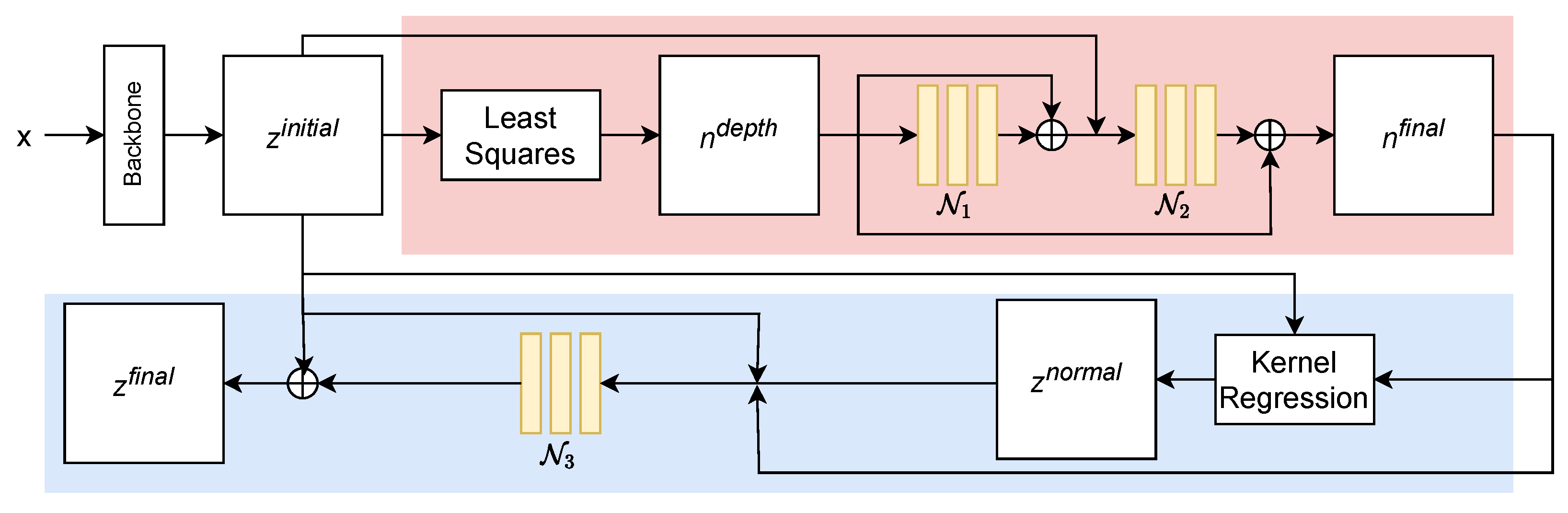
3.1. GeoNet
3.1.1. Normal Refinement
3.1.2. Depth Refinement
3.2. General Depth Enhancement Network
3.3. Loss Functions
3.4. Implementation Details
4. Training and Tasks
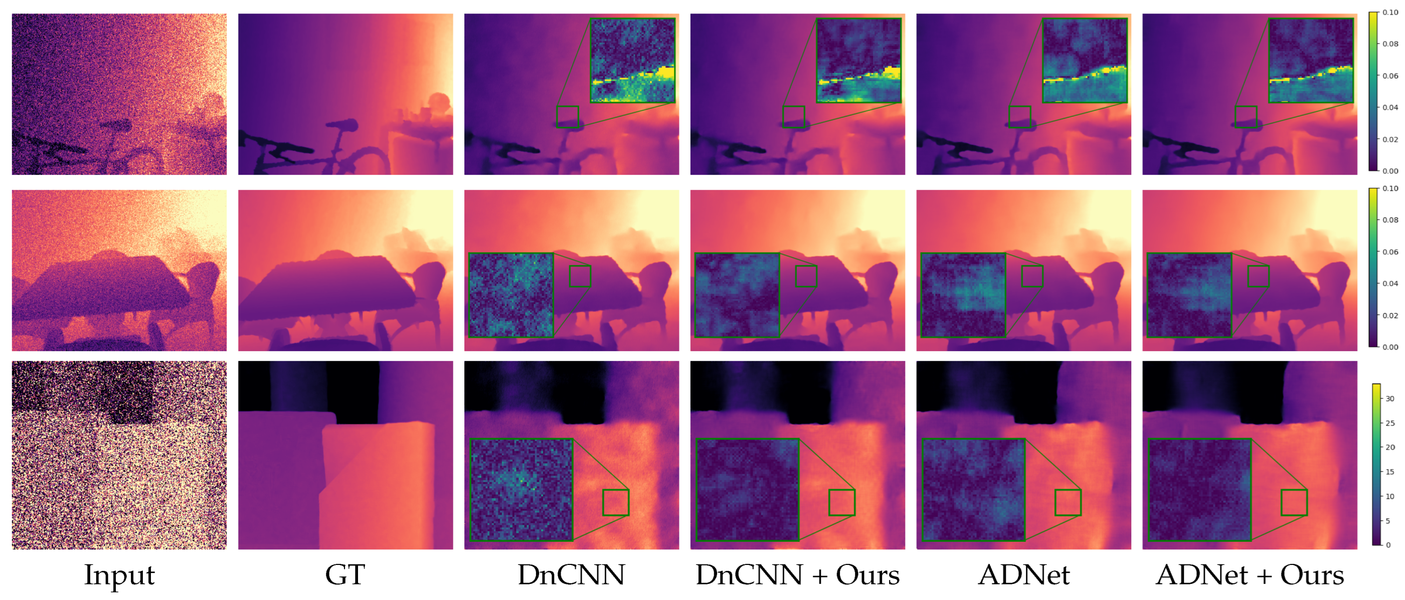
4.1. Denoising
4.2. Deblurring
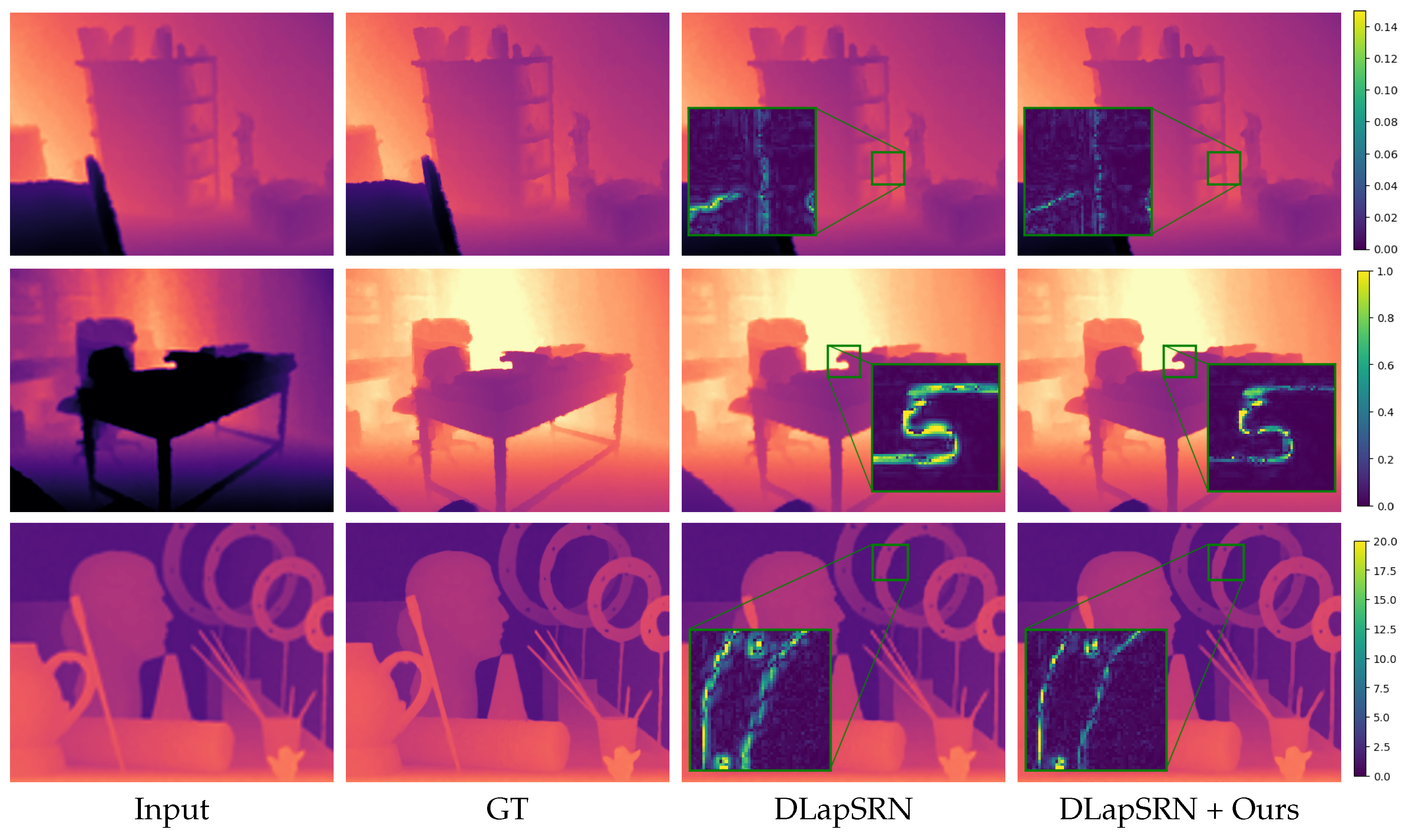
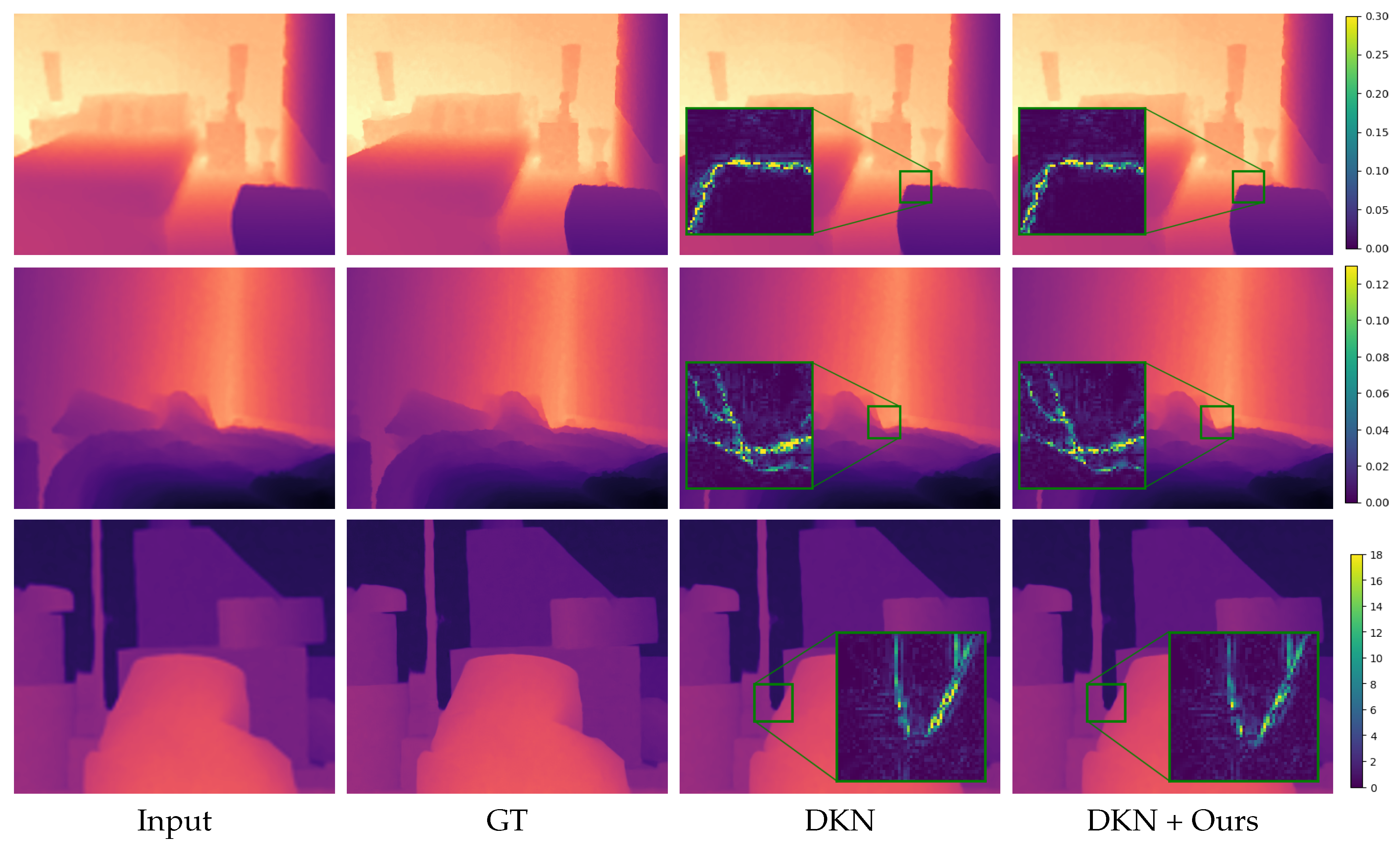
4.3. Super-Resolution
5. Results
6. Conclusions
Author Contributions
Funding
Institutional Review Board Statement
Informed Consent Statement
Data Availability Statement
Acknowledgments
Conflicts of Interest
Abbreviations
| CNN | Convolutional neural network |
| GAN | Generative Adversarial Neural Network |
| DnCNN | Denoising CNN |
| ADNet | Attention-guided denoising network |
| (D)LapSRN | (Depth) Laplacian pyramid super-resolution network |
| DKN | Deformable kernel network |
References
- Keller, M.; Lefloch, D.; Lambers, M.; Izadi, S.; Weyrich, T.; Kolb, A. Real-time 3d reconstruction in dynamic scenes using point-based fusion. In Proceedings of the 2013 International Conference on 3D Vision-3DV, Seattle, WA, USA, 29 June–1 July 2013; IEEE: Piscataway, NJ, USA, 2013; pp. 1–8. [Google Scholar]
- Dai, A.; Nießner, M.; Zollhöfer, M.; Izadi, S.; Theobalt, C. Bundlefusion: Real-time globally consistent 3d reconstruction using on-the-fly surface reintegration. ACM Trans. Graph. (ToG) 2017, 36, 1. [Google Scholar] [CrossRef]
- Lee, W.; Park, N.; Woo, W. Depth-assisted real-time 3D object detection for augmented reality. In Proceedings of the ICAT, Osaka, Japan, 28–30 November 2011; Volume 11, pp. 126–132. [Google Scholar]
- Holynski, A.; Kopf, J. Fast depth densification for occlusion-aware augmented reality. ACM Trans. Graph. (ToG) 2018, 37, 1–11. [Google Scholar] [CrossRef] [Green Version]
- Du, R.; Turner, E.; Dzitsiuk, M.; Prasso, L.; Duarte, I.; Dourgarian, J.; Afonso, J.; Pascoal, J.; Gladstone, J.; Cruces, N.; et al. DepthLab: Real-time 3D interaction with depth maps for mobile augmented reality. In Proceedings of the 33rd Annual ACM Symposium on User Interface Software and Technology, Virtual Event, 20–23 October 2020; pp. 829–843. [Google Scholar]
- You, Y.; Wang, Y.; Chao, W.L.; Garg, D.; Pleiss, G.; Hariharan, B.; Campbell, M.; Weinberger, K.Q. Pseudo-lidar++: Accurate depth for 3d object detection in autonomous driving. arXiv 2019, arXiv:1906.06310. [Google Scholar]
- Liao, M.; Lu, F.; Zhou, D.; Zhang, S.; Li, W.; Yang, R. Dvi: Depth guided video inpainting for autonomous driving. In Proceedings of the European Conference on Computer Vision, Glasgow, UK, 23–28 August 2020; Springer: Berlin/Heidelberg, Germany, 2020; pp. 1–17. [Google Scholar]
- Aladem, M.; Rawashdeh, S.A. A single-stream segmentation and depth prediction CNN for autonomous driving. IEEE Intell. Syst. 2020, 36, 79–85. [Google Scholar] [CrossRef]
- Steiner, H.; Sommerhoff, H.; Bulczak, D.; Jung, N.; Lambers, M.; Kolb, A. Fast motion estimation for field sequential imaging: Survey and benchmark. Image Vis. Comput. 2019, 89, 170–182. [Google Scholar] [CrossRef]
- Riegler, G.; Rüther, M.; Bischof, H. Atgv-net: Accurate depth super-resolution. In Proceedings of the European Conference on Computer Vision, Amsterdam, The Netherlands, 11–14 October 2016; Springer: Berlin/Heidelberg, Germany, 2016; pp. 268–284. [Google Scholar]
- Li, J.; Gao, W.; Wu, Y. High-quality 3d reconstruction with depth super-resolution and completion. IEEE Access 2019, 7, 19370–19381. [Google Scholar] [CrossRef]
- Hui, T.W.; Loy, C.C.; Tang, X. Depth map super-resolution by deep multi-scale guidance. In Proceedings of the European Conference on Computer Vision, Amsterdam, The Netherlands, 11–14 October 2016; Springer: Berlin/Heidelberg, Germany, 2016; pp. 353–369. [Google Scholar]
- Kim, B.; Ponce, J.; Ham, B. Deformable kernel networks for joint image filtering. Int. J. Comput. Vis. 2021, 129, 579–600. [Google Scholar] [CrossRef]
- Tang, J.; Chen, X.; Zeng, G. Joint implicit image function for guided depth super-resolution. In Proceedings of the 29th ACM International Conference on Multimedia, Chengdu, China, 20–24 October 2021; pp. 4390–4399. [Google Scholar]
- Guo, C.; Li, C.; Guo, J.; Cong, R.; Fu, H.; Han, P. Hierarchical features driven residual learning for depth map super-resolution. IEEE Trans. Image Process. 2018, 28, 2545–2557. [Google Scholar] [CrossRef] [PubMed]
- Sterzentsenko, V.; Saroglou, L.; Chatzitofis, A.; Thermos, S.; Zioulis, N.; Doumanoglou, A.; Zarpalas, D.; Daras, P. Self-supervised deep depth denoising. In Proceedings of the IEEE/CVF International Conference on Computer Vision, Seoul, Korea, 27–28 October 2019; pp. 1242–1251. [Google Scholar]
- Yan, S.; Wu, C.; Wang, L.; Xu, F.; An, L.; Guo, K.; Liu, Y. Ddrnet: Depth map denoising and refinement for consumer depth cameras using cascaded cnns. In Proceedings of the European Conference on Computer Vision (ECCV), Munich, Germany, 8–14 September 2018; pp. 151–167. [Google Scholar]
- Tourani, S.; Mittal, S.; Nagariya, A.; Chari, V.; Krishna, M. Rolling shutter and motion blur removal for depth cameras. In Proceedings of the 2016 IEEE International Conference on Robotics and Automation (ICRA), Stockholm, Sweden, 16–21 May 2016; IEEE: Piscataway, NJ, USA, 2016; pp. 5098–5105. [Google Scholar]
- Li, L.; Pan, J.; Lai, W.S.; Gao, C.; Sang, N.; Yang, M.H. Dynamic scene deblurring by depth guided model. IEEE Trans. Image Process. 2020, 29, 5273–5288. [Google Scholar] [CrossRef] [PubMed]
- Qi, X.; Liao, R.; Liu, Z.; Urtasun, R.; Jia, J. Geonet: Geometric neural network for joint depth and surface normal estimation. In Proceedings of the IEEE Conference on Computer Vision and Pattern Recognition, Salt Lake City, UT, USA, 18–23 June 2018; pp. 283–291. [Google Scholar]
- Qi, X.; Liu, Z.; Liao, R.; Torr, P.H.; Urtasun, R.; Jia, J. Geonet++: Iterative geometric neural network with edge-aware refinement for joint depth and surface normal estimation. IEEE Trans. Pattern Anal. Mach. Intell. 2020, 44, 969–984. [Google Scholar] [CrossRef] [PubMed]
- Eigen, D.; Fergus, R. Predicting depth, surface normals and semantic labels with a common multi-scale convolutional architecture. In Proceedings of the IEEE International Conference on Computer Vision, Santiago, Chile, 7–13 December 2015; pp. 2650–2658. [Google Scholar]
- Xu, D.; Ouyang, W.; Wang, X.; Sebe, N. Pad-net: Multi-tasks guided prediction-and-distillation network for simultaneous depth estimation and scene parsing. In Proceedings of the IEEE Conference on Computer Vision and Pattern Recognition, Salt Lake City, UT, USA, 18–23 June 2018; pp. 675–684. [Google Scholar]
- Wang, P.; Shen, X.; Russell, B.; Cohen, S.; Price, B.; Yuille, A.L. Surge: Surface regularized geometry estimation from a single image. Adv. Neural Inf. Process. Syst. 2016, 29. [Google Scholar]
- Huhle, B.; Schairer, T.; Jenke, P.; Straßer, W. Robust non-local denoising of colored depth data. In Proceedings of the 2008 IEEE Computer Society Conference on Computer Vision and Pattern Recognition Workshops, Anchorage, AK, USA, 24–26 June 2008; IEEE: Piscataway, NJ, USA, 2008; pp. 1–7. [Google Scholar]
- Ferstl, D.; Reinbacher, C.; Ranftl, R.; Rüther, M.; Bischof, H. Image guided depth upsampling using anisotropic total generalized variation. In Proceedings of the IEEE International Conference on Computer Vision, Sydney, Australia, 1–8 December 2013; pp. 993–1000. [Google Scholar]
- Shen, J.; Cheung, S.C.S. Layer depth denoising and completion for structured-light rgb-d cameras. In Proceedings of the IEEE Conference on Computer Vision and Pattern Recognition, Portland, OR, USA, 23–28 June 2013; pp. 1187–1194. [Google Scholar]
- Fu, J.; Wang, S.; Lu, Y.; Li, S.; Zeng, W. Kinect-like depth denoising. In Proceedings of the 2012 IEEE International Symposium on Circuits and Systems (ISCAS), Seoul, Korea, 20–23 May 2012; IEEE: Piscataway, NJ, USA, 2012; pp. 512–515. [Google Scholar]
- Lai, W.S.; Huang, J.B.; Ahuja, N.; Yang, M.H. Deep laplacian pyramid networks for fast and accurate super-resolution. In Proceedings of the IEEE Conference on Computer Vision and Pattern Recognition, Honolulu, HI, USA, 21–26 July 2017; pp. 624–632. [Google Scholar]
- Zhao, L.; Bai, H.; Liang, J.; Zeng, B.; Wang, A.; Zhao, Y. Simultaneous color-depth super-resolution with conditional generative adversarial networks. Pattern Recognit. 2019, 88, 356–369. [Google Scholar] [CrossRef]
- Zhong, Z.; Liu, X.; Jiang, J.; Zhao, D.; Chen, Z.; Ji, X. High-Resolution Depth Maps Imaging via Attention-Based Hierarchical Multi-Modal Fusion. IEEE Trans. Image Process. 2021, 31, 648–663. [Google Scholar] [CrossRef] [PubMed]
- Charbonnier, P.; Blanc-Feraud, L.; Aubert, G.; Barlaud, M. Two deterministic half-quadratic regularization algorithms for computed imaging. In Proceedings of the 1st International Conference on Image Processing, Austin, TX, USA, 13–16 November 1994; IEEE: Piscataway, NJ, USA, 1994; Volume 2, pp. 168–172. [Google Scholar]
- Silberman, N.; Hoiem, D.; Kohli, P.; Fergus, R. Indoor Segmentation and Support Inference from RGBD Images. In Proceedings of the ECCV, Florence, Italy, 7–13 October 2012. [Google Scholar]
- Zhang, K.; Zuo, W.; Chen, Y.; Meng, D.; Zhang, L. Beyond a gaussian denoiser: Residual learning of deep cnn for image denoising. IEEE Trans. Image Process. 2017, 26, 3142–3155. [Google Scholar] [CrossRef] [PubMed] [Green Version]
- Tian, C.; Xu, Y.; Li, Z.; Zuo, W.; Fei, L.; Liu, H. Attention-guided CNN for image denoising. Neural Netw. 2020, 124, 117–129. [Google Scholar] [CrossRef] [PubMed]
- Wang, Z.; Bovik, A.C.; Sheikh, H.R.; Simoncelli, E.P. Image quality assessment: From error visibility to structural similarity. IEEE Trans. Image Process. 2004, 13, 600–612. [Google Scholar] [CrossRef] [PubMed] [Green Version]
- Hirschmuller, H.; Scharstein, D. Evaluation of cost functions for stereo matching. In Proceedings of the 2007 IEEE Conference on Computer Vision and Pattern Recognition, Minneapolis, MN, USA, 17–22 June 2007; IEEE: Piscataway, NJ, USA, 2007; pp. 1–8. [Google Scholar]
- He, K.; Zhang, X.; Ren, S.; Sun, J. Deep residual learning for image recognition. In Proceedings of the IEEE Conference on Computer Vision and Pattern Recognition, Las Vegas, NV, USA, 27–30 June 2016; pp. 770–778. [Google Scholar]


| Network | DnCNN | ADNet | ResNet | DLapSRN | DKN | +Ours |
| Parameters | 556K | 519K | 556K | 435K | 1.4M | +235K |
| Time (ms) | 26 | 28 | 26 | 10 | 126 | +34 |
| Task | Method | RMSE ↓ | MAE ↓ | SSIM ↑ |
|---|---|---|---|---|
| Denoising | DnCNN [34] | 4.07 | 2.84 | 0.9663 |
| DnCNN [34] + Ours | 3.81 | 2.57 | 0.9757 | |
| ADNet [35] | 3.64 | 2.47 | 0.9730 | |
| ADNet [35] + Ours | 3.55 | 2.34 | 0.9743 | |
| Deblurring | ResNet [38] | 3.14 | 2.14 | 0.9897 |
| ResNet [38] + Ours | 2.97 | 2.00 | 0.9896 | |
| Super-resolution (Depth only) | Bilinear | 3.63 | 1.09 | 0.9821 |
| Bilinear + Ours | 3.07 | 0.93 | 0.9849 | |
| DLapSRN [11] | 2.85 | 0.88 | 0.9863 | |
| DLapSRN [11] + Ours | 2.26 | 0.71 | 0.9889 | |
| Super-resolution (RGB guided) | DKN [13] | 1.68 | 0.61 | 0.9931 |
| DKN [13] + Ours | 1.59 | 0.59 | 0.9936 |
| Task | Method | RMSE ↓ | MAE ↓ | SSIM ↑ |
|---|---|---|---|---|
| Denoising | DnCNN [34] | 6.21 | 4.49 | 0.8932 |
| DnCNN [34] + Ours | 5.55 | 3.82 | 0.9427 | |
| ADNet [35] | 5.32 | 3.70 | 0.9200 | |
| ADNet [35] + Ours | 5.09 | 3.44 | 0.9383 | |
| Deblurring | ResNet [38] | 3.06 | 1.74 | 0.9574 |
| ResNet [38] + Ours | 2.96 | 1.67 | 0.9581 | |
| Super-resolution (Depth only) | Bilinear | 2.54 | 1.00 | 0.9629 |
| Bilinear + Ours | 2.35 | 0.93 | 0.9663 | |
| DLapSRN [11] | 2.03 | 0.85 | 0.9696 | |
| DLapSRN [11] + Ours | 1.69 | 0.74 | 0.9749 | |
| Super-resolution (RGB guided) | DKN [13] | 1.23 | 0.61 | 0.9805 |
| DKN [13] + Ours | 1.09 | 0.60 | 0.9806 |
Publisher’s Note: MDPI stays neutral with regard to jurisdictional claims in published maps and institutional affiliations. |
© 2022 by the authors. Licensee MDPI, Basel, Switzerland. This article is an open access article distributed under the terms and conditions of the Creative Commons Attribution (CC BY) license (https://creativecommons.org/licenses/by/4.0/).
Share and Cite
Sommerhoff, H.; Kolb, A. A Generic Framework for Depth Reconstruction Enhancement. J. Imaging 2022, 8, 138. https://doi.org/10.3390/jimaging8050138
Sommerhoff H, Kolb A. A Generic Framework for Depth Reconstruction Enhancement. Journal of Imaging. 2022; 8(5):138. https://doi.org/10.3390/jimaging8050138
Chicago/Turabian StyleSommerhoff, Hendrik, and Andreas Kolb. 2022. "A Generic Framework for Depth Reconstruction Enhancement" Journal of Imaging 8, no. 5: 138. https://doi.org/10.3390/jimaging8050138
APA StyleSommerhoff, H., & Kolb, A. (2022). A Generic Framework for Depth Reconstruction Enhancement. Journal of Imaging, 8(5), 138. https://doi.org/10.3390/jimaging8050138