Technical Note

Self-Supervised Learning of Satellite-Derived Vegetation Indices for Clustering and Visualization of Vegetation Types

Department of Informatics, Tokyo University of Information Sciences, 4-1 Onaridai, Wakaba-ku, Chiba 265-8501, Japan
*
Author to whom correspondence should be addressed.
J. Imaging 2021, 7(2), 30; https://doi.org/10.3390/jimaging7020030
Submission received: 27 September 2020 / Revised: 13 January 2021 / Accepted: 25 January 2021 / Published: 8 February 2021

Abstract

:
Vegetation indices are commonly used techniques for the retrieval of biophysical and chemical attributes of vegetation. This paper presents the potential of an Autoencoders (AEs) and Convolutional Autoencoders (CAEs)-based self-supervised learning approach for the decorrelation and dimensionality reduction of high-dimensional vegetation indices derived from satellite observations. This research was implemented in Mt. Zao and its base in northeast Japan with a cool temperate climate by collecting the ground truth points belonging to 16 vegetation types (including some non-vegetation classes) in 2018. Monthly median composites of 16 vegetation indices were generated by processing all Sentinel-2 scenes available for the study area from 2017 to 2019. The performance of AEs and CAEs-based compressed images for the clustering and visualization of vegetation types was quantitatively assessed by computing the bootstrap resampling-based confidence interval. The AEs and CAEs-based compressed images with three features showed around 4% and 9% improvements in the confidence intervals respectively over the classical method. CAEs using convolutional neural networks showed better feature extraction and dimensionality reduction capacity than the AEs. The class-wise performance analysis also showed the superiority of the CAEs. This research highlights the potential of AEs and CAEs for attaining a fine clustering and visualization of vegetation types.

1. Introduction

Vegetation is an integral component of life, and identification and classification of vegetation types provides valuable information for understanding the distribution and dynamics of vegetation as for environmental changes. Spectral reflectance measured from remote sensing platforms provides crucial information on identification and discrimination of vegetation types.
The reflectance measured from remote sensors vary with specific biophysical and chemical attributes such as plant type, leaf pigments, water content, and morphological characteristics of the plant canopy concerned [1,2]. Vegetation indices, arithmetic combination of reflectance in multiple wavelengths, have been derived for detecting the biophysical and chemical attributes of vegetation [3]. The vegetation indices are commonly utilized for monitoring and evaluation of extent and coverage of vegetation types [4,5]. However, a large number of vegetation indices exist in the literature, and large numbers of input variables complicate modelling and prediction, and impairs accuracy, known as the “curse of dimensionality” [6,7]. To cope with this problem, dimensionality reduction techniques, which transform high-dimensional dataset into lower-dimensional representations have been proposed [8,9].
Machine learning is a commonly used technique for interpreting remote sensing images into vegetation parameters. There are a number of machine learning algorithms available for dimensionality reductions. The Random Forests (RFs)—an ensemble of decision trees built by splitting the attributes of the data and averaging the output value of all trees—is one of the effective machine learning algorithms for learning non-linear data interactions [10,11]. The RF algorithm also provides an effective statistical measure for determining variable importance [12,13,14]. Researchers have utilized the RFs-based retrieval of important variables as a measure of reducing the dimensions of data [15,16,17,18] and classification of land cover and vegetation types [19,20,21].
Some other classical techniques of dimensionality reductions are principal component analysis [22,23,24], t-distributed stochastic neighbor embedding [25,26], and modified stochastic neighbor embedding [27] as some examples. Oliveira et al. [28] assessed the performance of classical techniques and proposed fractal-based algorithm to remove the redundant attributes accurately.
Artificial neural networks (ANNs) has demonstrated effectiveness in a number of climate change and ecological studies, such as change detection [29], plant identification [30,31], modeling the distribution of vegetation in past, present, and future climates [32], estimation of standing crop and fuel moisture content [33], and mixture estimation for vegetation mapping [34] as some examples.
In recent years, the use of Autoencoders (AEs) has attracted increasing attention to create low-dimensional projections of high-dimensional data. AEs are artificial neural networks (ANNs) designed for learning self-supervised latent representations of multi-dimensional data [35,36,37].The AEs provides a latent-space representation with a reduced dimensionality through the process of compressing (encoding) and decompressing (decoding) of the multi-dimensional data [38,39].
The major objective of this paper is to present an Autoencoders (AEs) and Convolutional Autoencoders (CAEs)-based self-supervised learning approach for the decorrelation and dimensionality reduction of high-dimensional vegetation indices derived from satellite observations. The compressed images are utilized for the clustering and visualization of vegetation types, and they were compared over the Random Forests-based important features. The potential of this approach for the classification of vegetation types is also assessed using the Random Forests (RFs) classifier.

2. Materials and Methods

2.1. Study Area

This research was implemented in Mt. Zao, which is located on the border between Yamagata and Miyagi prefectures in Japan. This region is characterized by a cool temperate climate with snowfall during winter. It represents a typical mountainous ecosystem in northeastern Japan. The location of the study area is shown in Figure 1.

2.2. Collection of Ground Truth Data

The performance of Autoencoders (AEs) and Convolutional Autoencoders (CAEs) for the clustering and classification of vegetation types was assessed with the support of ground truth data. The ground truth data were collected through a field survey, which was conducted in 2018. The field survey was assisted by time-lapse images available in Google Earth. For each vegetation type, 107–300 sample points (longitudes and latitudes), representing a homogenous area of at least 30 × 30 m, were collected. This research dealt with the following list of vegetation types (Table 1) present in the study region.

2.3. Processing of Satellite Data

Sentinel-2 scenes available for the study area from 2017 to 2019 (total 343 scenes) were processed. All images were processed for cloud removal and atmospherically corrected to obtain top of canopy reflectance using the Sen2Cor software (v2.8). For each Sentinel-2 scene, 16 vegetation indices (as shown in Table 2) were calculated, and the resulting vegetation index images were composited by computing monthly median values. In this manner, we obtained a monthly stack of vegetation index images, consisting of 192 (16 vegetation indices × 12 months) layers.

2.4. Dimensionality Reduction

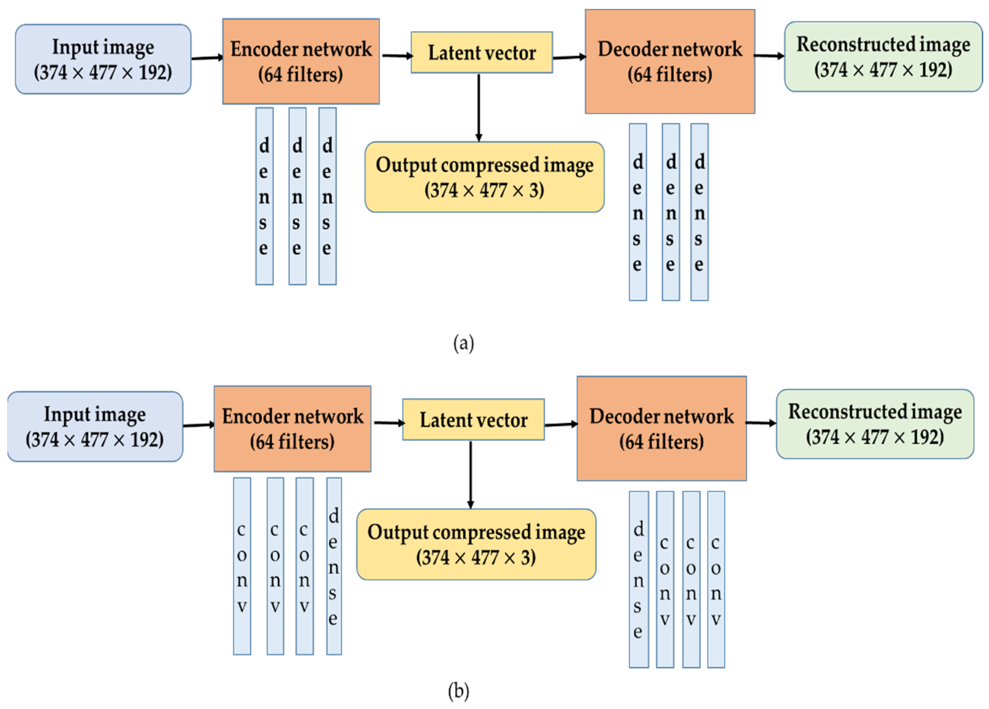
We employed densely connected Autoencoders (AEs) and Convolutional Autoencoders (CAEs) for the decorrelation of high-dimensional vegetation indices. The model architectures utilized in this research are illustrated in Figure 2. The 192-dimensional stack of vegetation indices was fed into AEs and CAEs models. The AEs were composed of three dense layers; whereas the CAEs were composed of three convolutional layers, and a fully connected (dense) layer was used to collect the outputs from the final convolutional layer. Finally, multiple (3, 5, and 10) low-dimensional latent vectors were obtained from the final dense layer. For the self-supervised learning, we split the dataset into training (95%) and testing (5%) to tune the parameters and hyper-parameters of the models such as the learning rate, number of epochs, and batch size through a repeated trial and error process.

2.5. Quantitative Evaluation

The performance of AEs and CAEs-based compressed images for the clustering and visualization was compared to the classical RFs-based retrieval of the important features. The RFs algorithm has been employed as a classical approach for deriving variable importance [55]. The pixel values, corresponding to the ground truth (geolocation points) data, for each vegetation type were extracted from the compressed images (AEs, CAEs, and RFs) and utilized for the visualization and classification of vegetation types. We used 3D scatter plots to visualize the clusters of vegetation types and employed the RFs classifier for the classification of vegetation types.
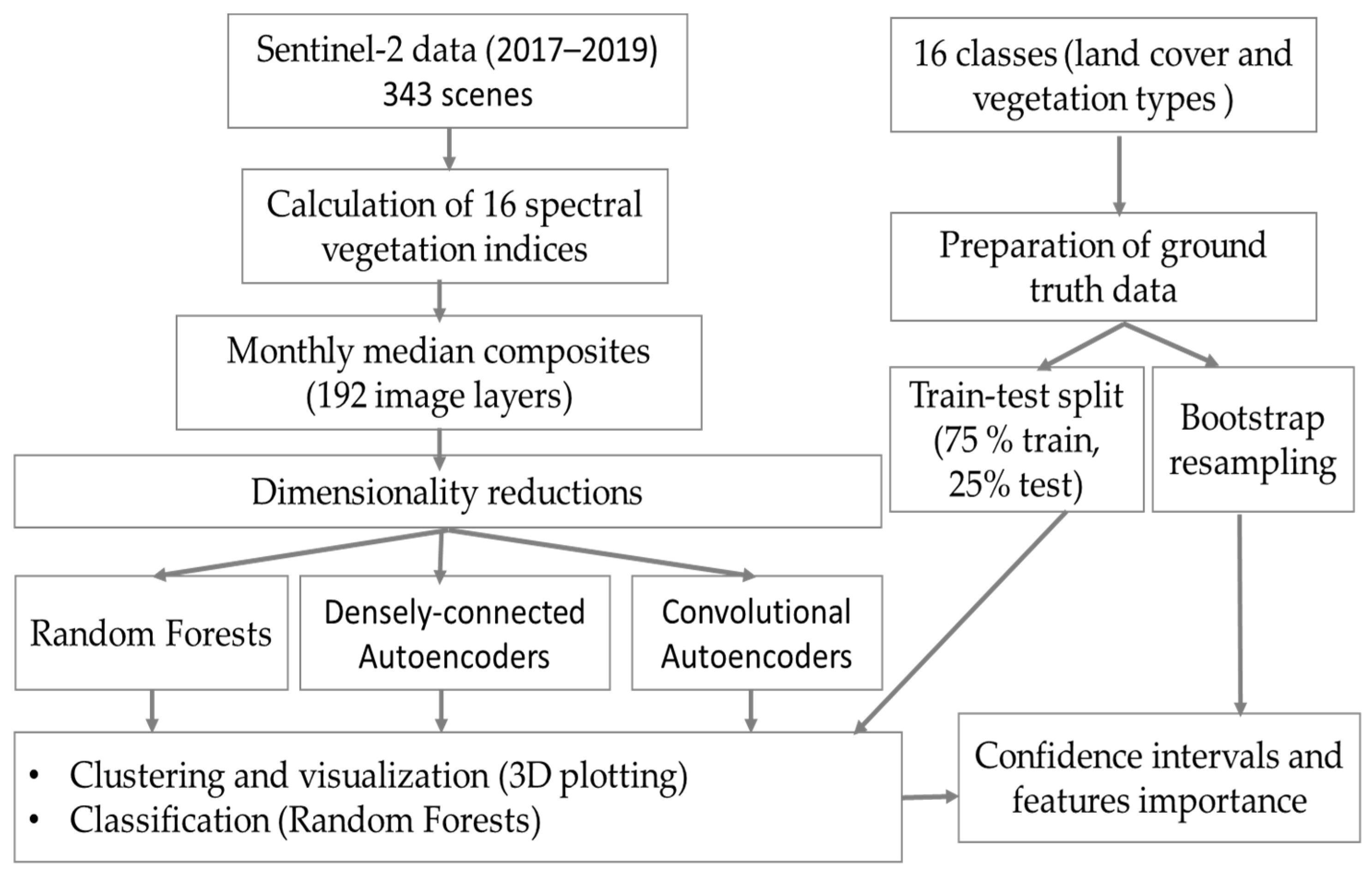
Furthermore, performance of the compressed images (AEs, CAEs, and RFs) in different dimensions (3, 5, and 10) in terms of classification of vegetation types was also assessed quantitatively. For the supervised classification, Random Forests (RFs) classifier was employed on a 75% training set and validated on a 25% test set. For the quantitative evaluation, we computed the confidence interval by implementing bootstrap resampling of the dataset at 1000 times. The bootstrap resampling technique involves drawing of sample data repeatedly with replacement from a data source and reduces a biased estimation of the accuracy. The research procedure has been illustrated in Figure 3.

3. Results

3.1. Clustering and Visualization

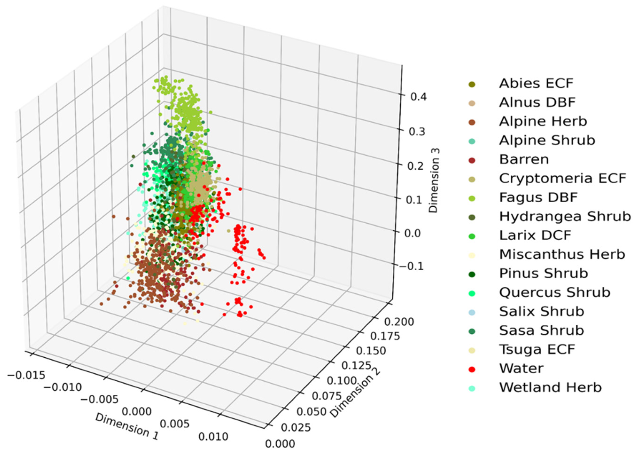
The discriminative ability of the lower dimensional features can be visualized by plotting their distribution in a three-dimensional space. A three-dimensional scatter plot of the RFs algorithm-based retrieval of the most important features is shown in Figure 4. As seen in the figure, most of the inter-class clusters are closed to each other. Therefore, it indicates shortcomings of the RFs-based important features on distinguishing most of the vegetation types.
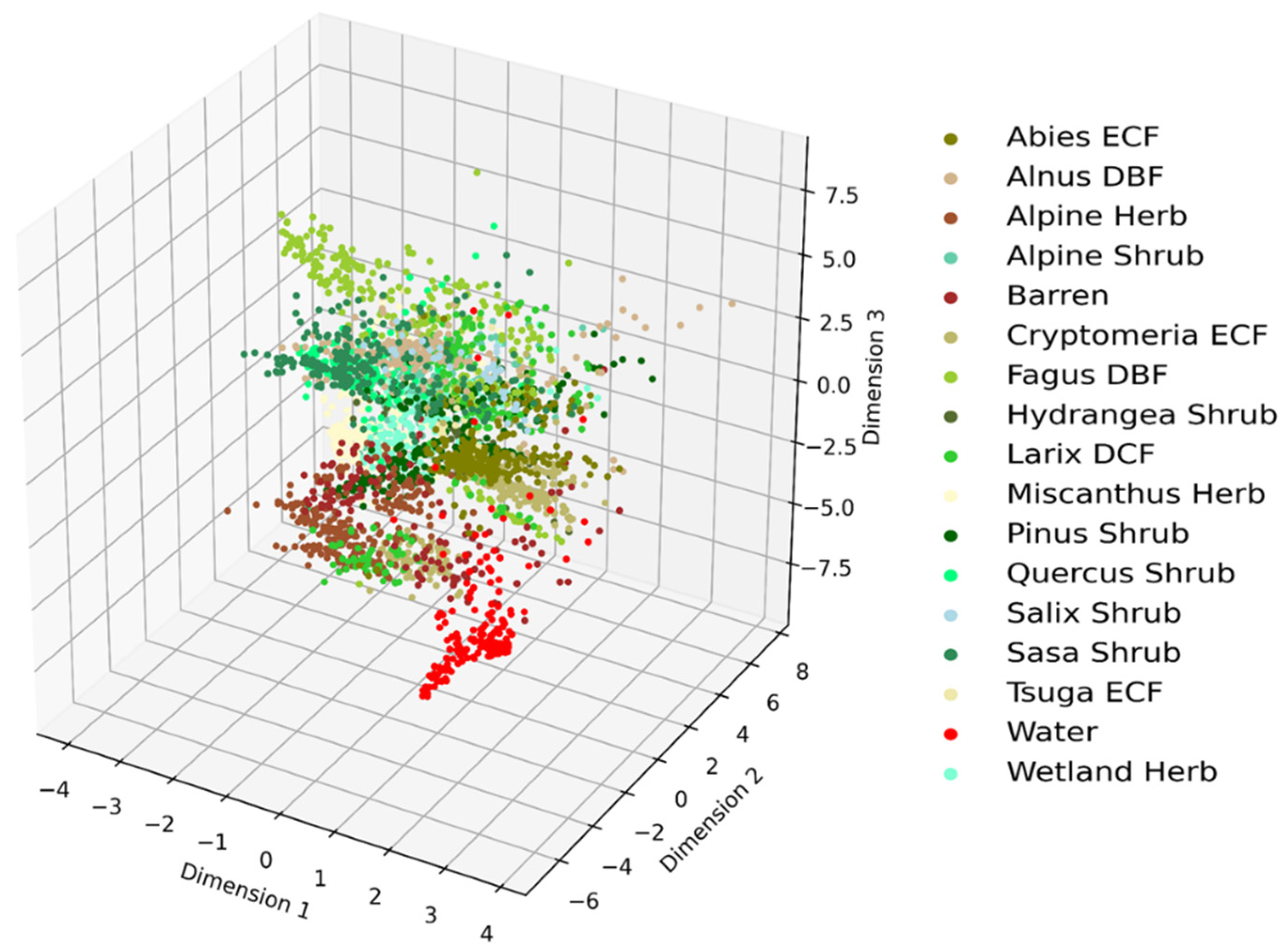
An improvement on the clustering of vegetation types by the AEs-based compressed features over the RFs algorithm can be seen with a wider inter-class variation of the clusters in Figure 5.
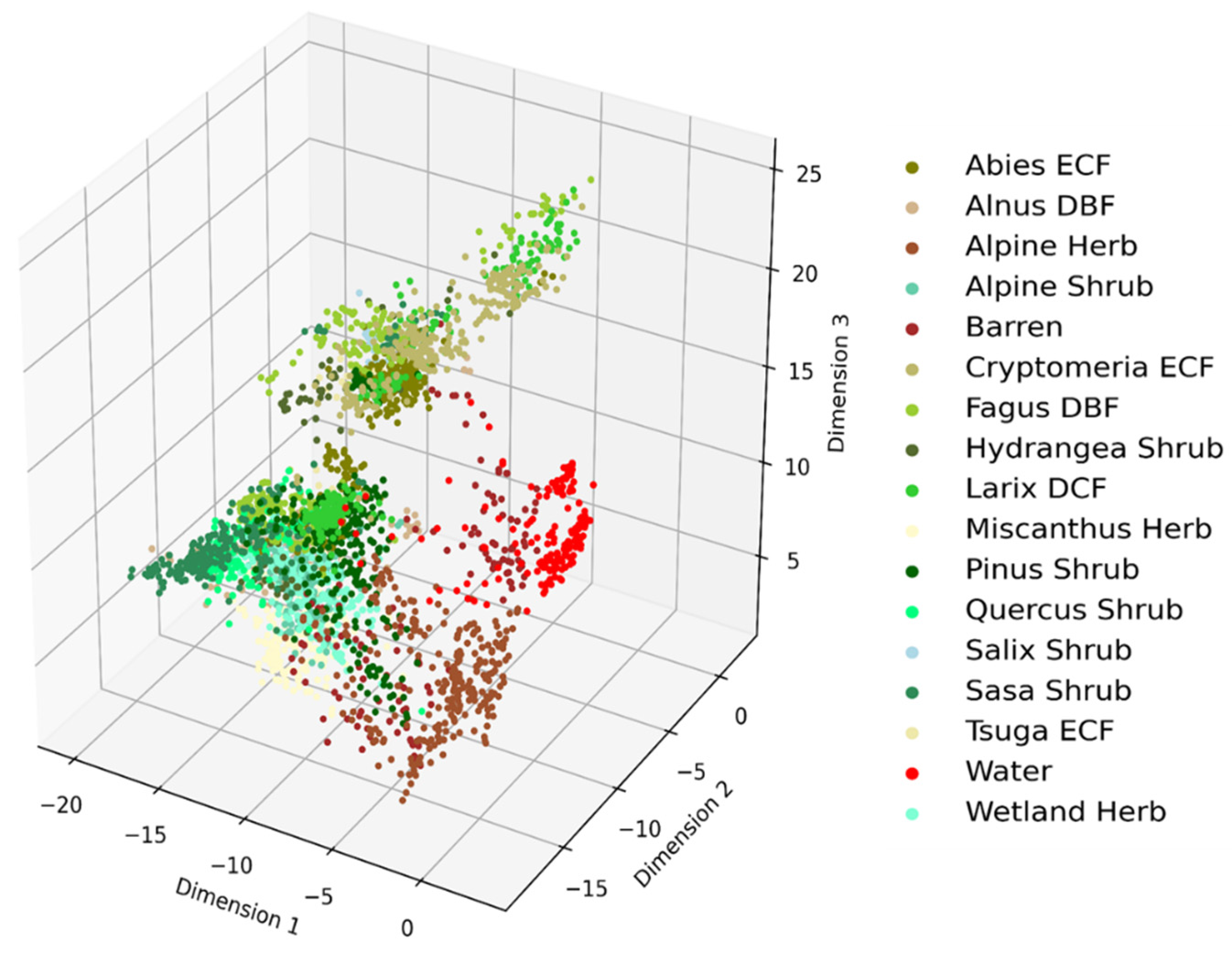
Further improvement by the CAEs-based compressed features can be seen in Figure 6. The 3D cluster shows its ability to distinguish vegetation types that were not distinguished by RFs-based important features.
The RGB color composites of the AEs and CAEs-based three-dimensional compressed images in Figure 7 demonstrate a variation of color shades over different vegetation types. Generating distinct color shades for different vegetation types under the study is crucial for the improved discrimination and classification with the least number of input features.

3.2. Confidence Intervals

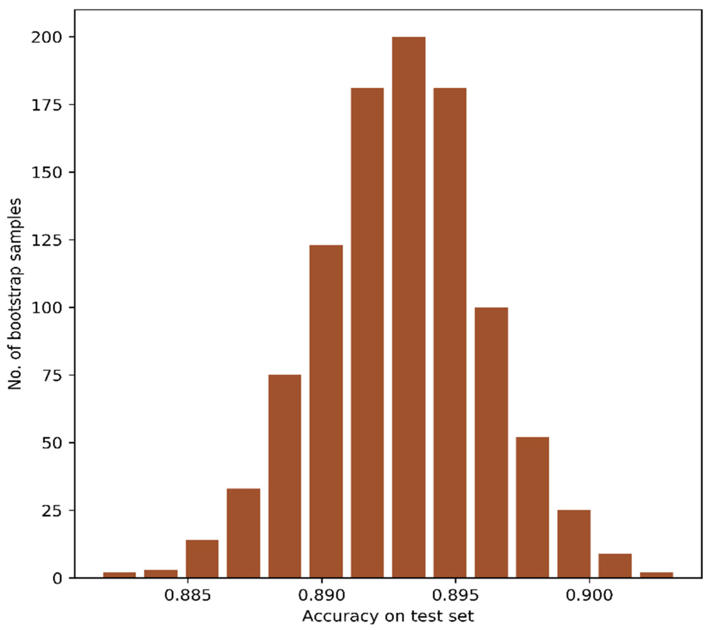
We employed the bootstrap resampling method to report the confidence interval of the CAEs-based classification approach. The bootstrap resampling was done for 1000 times with 75% training and 25% testing data. The accuracy obtained with the test data was collected for each bootstrap resampling, and the frequency of models yielding the test accuracies has been plotted in Figure 8. We also computed the accuracy at a 95% confidence interval. The CAEs-based three features provided test accuracy between 88.7% and 89.9% with a 95.0% confidence interval.
The distribution of feature importance obtained from bootstrap resampling of the CAEs-based three features has been shown in Figure 9. For each bootstrap resampling, the features distribution showed positive contribution to the model.
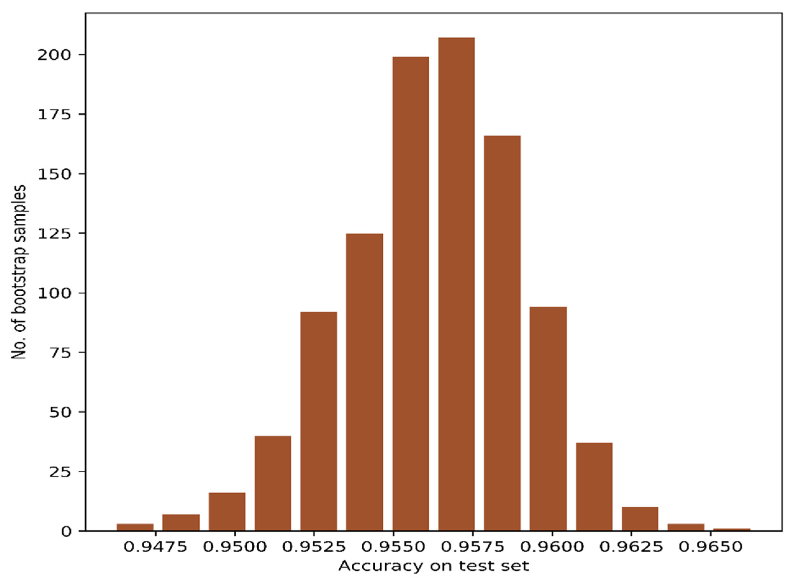
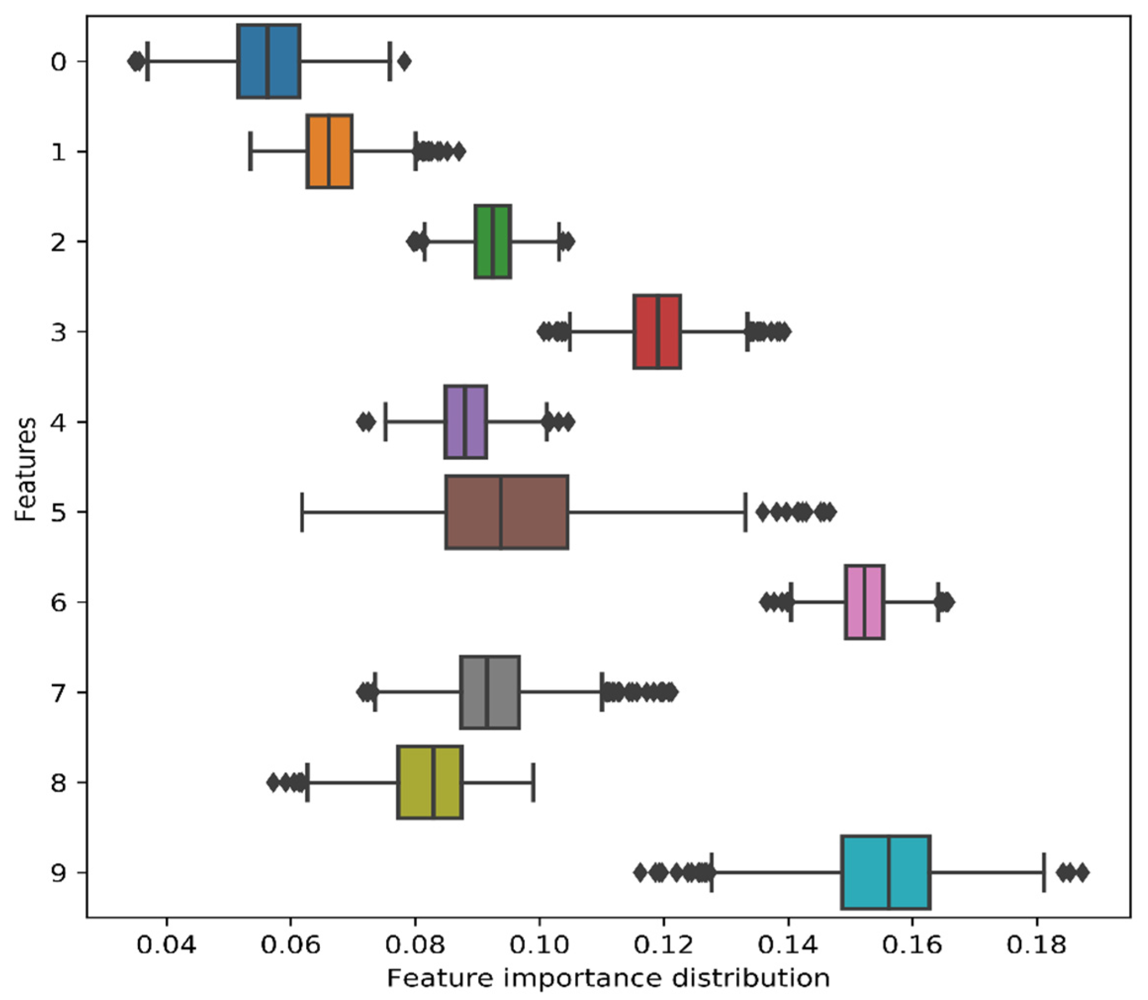
Similarly, we calculated the test accuracy using ten features obtained from the CAEs, and the frequency of models yielding the test accuracies has been plotted in Figure 10. The CAEs-based ten features provided test accuracy between 95.0% and 96.2% with a 95.0% confidence interval. In addition, for each bootstrap resampling, the features distribution (10 features) showed positive contribution to the model (Figure 11).
Furthermore, we summarized the significance of the Autoencoders (AEs) and Convolutional Autoencoders (CAEs) over the Random Forests (RFs) by employing bootstrap resampling at 1000 times with 75% training and 25% testing data. Table 3 shows test accuracies computed with a 0.95 confidence interval.
The test accuracies obtained from the bootstrap resampling also showed a higher performance of the Autoencoders (AEs) and Convolutional Autoencoders (CAEs) over the Random Forests (RFs). Interestingly, it should be noted that difference between them (RFs versus AEs or CAEs) started to decrease when number of input features increased. However, the main objective of this research was to compress the high-dimensional dataset into least dimension so as to visualize the inter-class variability of the vegetation types. Therefore, self-supervised learning with the Autoencoders (AEs) and Convolutional Autoencoders (CAEs) has met our objective of showing the inter-class variability of vegetation types at lower dimension. The collection and preparation of ground truth data is very time-consuming and expensive for the vegetation mapping projects. The ability of such self-supervised learning and visualization of the satellite images should contribute to the better interpretation and discrimination of vegetation types (such as collection of ground truth data) as well as subsequent supervised classification for the operational mapping of vegetation types at a broad scale.

4. Discussion

We implemented the Autoencoders (AEs) and Convolutional Autoencoders (CAEs)-based self-supervised learning approach for the decorrelation and dimensionality reduction of high-dimensional satellite-based features. Deep learning is a versatile technology specialized for big datasets. Once the high-dimensional features were compressed into lower ones, we employed Random Forests (RFs) classifier for the classification of vegetation types.
A significant processing challenge exists with an ever-increasing collection of huge volumes of remote sensing data with enhanced spatial and spectral resolution. To address this issue, dimensionality reduction techniques have been recommended for reducing the complexity of the data while retaining the relevant information for the analysis [56,57]. Therefore, dimensionality reduction of high-dimensional vegetation indices is a relevant technique, while a large number of vegetation indices exist in the literature.
Spectral vegetation indices have been used by many researchers for the clustering and classification of vegetation types. For example, Villoslada et al. [58] highlighted the need to utilize a wide array of vegetation indices for the improved classification of vegetation types in coastal wetlands. Similarly, Kobayashi et al. [59] utilized spectral indices calculated from a Sentinel-2 multispectral instrument for crop classification. Wang et al. [60] used Fourier transforms on multi-temporal vegetation indices for unsupervised clustering of crop types. These researches motivated us to conduct the clustering and classification of sixteen vegetation types (including non-vegetation classes) solely based on vegetation indices.
Previous studies have also attempted dimensionality reduction of remote sensing data for the classification and mapping of vegetation types. However, most of these researchers have employed classical dimensionality reduction techniques. For example, Alaibakhsh et al. [61] used Principal component analysis (PCA) to delineate riparian vegetation from Landsat multi-temporal imagery. Similarly, Dadon et al. [62] used an improved PCA-based classification scheme to classify Mediterranean forest types in an unsupervised way. The t-Distributed Stochastic Neighbor Embedding (t-SNE) algorithm has been used to strengthen the quality of ground truth data used in the mapping of heterogeneous vegetation [63]. Some researchers have used self-organizing feature maps for the classification of crop types [64,65]. In this context, exploring the potential of deep, self-supervised learning approaches for the clustering and visualization of vegetation types is a timely and important research.

5. Conclusions

In this research, we showed Autoencoders (AEs)-based self-supervised learning as a potential approach for the decorrelation and compression of high-dimensional vegetation indices in a cool temperate mountainous ecosystem in Japan. Compared to the classical Random Forests (RFs)-based dimensionality reduction method, the Autoencoders (AEs) and Convolutional Autoencoders (CAEs) showed superior performance on the clustering and classification of vegetation types. While the purpose of dimensionality reduction approaches is to represent the relevant information into the least amount of dimensions, the three-dimensional compression of vegetation indices using the CAEs method showed around a 9% increase in the confidence interval over the RFs. The RFs extracts the most important features out of given features, whereas the AEs and CAEs generate compressed features through self-supervised learning approach. Therefore, this research highlights the application of the CAEs method for the clustering and visualization of vegetation types. In the future, we will assess the efficiency of CAEs in other regions.

Author Contributions

R.C.S. performed research and wrote the manuscript. K.H. supervised the research and revised the manuscript. Both authors have read and agreed to the published version of the manuscript.

Funding

This research was partially funded by JSPS KAKENHI (Grant-in-Aid for Scientific Research) JP19H04320. The field data was supported by the commissioned research of the Ministry of the Environment, Centre for Biodiversity and Asia Air Survey Co., Ltd.

Institutional Review Board Statement

Not applicable.

Informed Consent Statement

Not applicable.

Data Availability Statement

Not applicable.

Acknowledgments

Authors are thankful to anonymous reviewers and editors of the Journal. Sentinel-2 data were available from the European Space Agency (ESA) Copernicus Open Access Hub.

Conflicts of Interest

The authors declare no conflict of interest.

References

  1. Ustin, S.L.; Gamon, J.A. Remote sensing of plant functional types: Tansley review. New Phytol. 2010, 186, 795–816. [Google Scholar] [CrossRef]
  2. Deepak, M.; Keski-Saari, S.; Fauch, L.; Granlund, L.; Oksanen, E.; Keinänen, M. Leaf canopy layers affect spectral reflectance in silver birch. Remote Sens. 2019, 11, 2884. [Google Scholar] [CrossRef] [Green Version]
  3. Bannari, A.; Morin, D.; Bonn, F.; Huete, A.R. A review of vegetation indices. Remote Sens. Rev. 1995, 13, 95–120. [Google Scholar] [CrossRef]
  4. Teillet, P. Effects of spectral, spatial, and radiometric characteristics on remote sensing vegetation indices of forested regions. Remote Sens. Environ. 1997, 61, 139–149. [Google Scholar] [CrossRef]
  5. Xue, J.; Su, B. Significant remote sensing vegetation indices: A review of developments and applications. J. Sens. 2017, 2017, 1–17. [Google Scholar] [CrossRef] [Green Version]
  6. Bach, F. Breaking the curse of dimensionality with convex neural networks. J. Mach. Learn. Res. 2017, 18, 629–681. [Google Scholar]
  7. Poggio, T.; Mhaskar, H.; Rosasco, L.; Miranda, B.; Liao, Q. Why and when can deep-but not shallow-networks avoid the curse of dimensionality: A review. Int. J. Autom. Comput. 2017, 14, 503–519. [Google Scholar] [CrossRef] [Green Version]
  8. Yan, W.; Sun, Q.; Sun, H.; Li, Y.; Ren, Z. Multiple kernel dimensionality reduction based on linear regression virtual reconstruction for image set classification. Neurocomputing 2019, 361, 256–269. [Google Scholar] [CrossRef]
  9. Reddy, G.T.; Reddy, M.P.K.; Lakshmanna, K.; Kaluri, R.; Rajput, D.S.; Srivastava, G.; Baker, T. Analysis of dimensionality reduction techniques on big data. IEEE Access 2020, 8, 54776–54788. [Google Scholar] [CrossRef]
  10. Breiman, L. Random forests. Mach. Learn. 2001, 45, 5–32. [Google Scholar] [CrossRef] [Green Version]
  11. Biau, G. Analysis of a random forests model. J. Mach. Learn. Res. 2012, 13, 1063–1095. [Google Scholar]
  12. Archer, K.J.; Kimes, R.V. Empirical characterization of random forest variable importance measures. Comput. Stat. Data Anal. 2008, 52, 2249–2260. [Google Scholar] [CrossRef]
  13. Genuer, R.; Poggi, J.-M.; Tuleau-Malot, C. Variable selection using random forests. Pattern Recognit. Lett. 2010, 31, 2225–2236. [Google Scholar] [CrossRef] [Green Version]
  14. Behnamian, A.; Millard, K.; Banks, S.N.; White, L.; Richardson, M.; Pasher, J. A systematic approach for variable selection with random forests: Achieving stable variable importance values. IEEE Geosci. Remote Sens. Lett. 2017, 14, 1988–1992. [Google Scholar] [CrossRef] [Green Version]
  15. Poona, N.K.; Ismail, R. Reducing hyperspectral data dimensionality using random forest based wrappers. In Proceedings of the 2013 IEEE International Geoscience and Remote Sensing Symposium—IGARSS, Melbourne, VIC, Australia, 21–26 July 2013; pp. 1470–1473. [Google Scholar]
  16. Belgiu, M.; Drăguţ, L. Random forest in remote sensing: A review of applications and future directions. ISPRS J. Photogramm. Remote Sens. 2016, 114, 24–31. [Google Scholar] [CrossRef]
  17. Lefkovits, L.; Lefkovits, S.; Emerich, S.; Vaida, M.F. Random Forest Feature Selection Approach for Image Segmentation; Verikas, A., Radeva, P., Nikolaev, D.P., Zhang, W., Zhou, J., Eds.; SPIE: Bellingham, WA, USA, 2017; p. 1034117. [Google Scholar]
  18. Gilbertson, J.K.; van Niekerk, A. Value of dimensionality reduction for crop differentiation with multi-temporal imagery and machine learning. Comput. Electron. Agric. 2017, 142, 50–58. [Google Scholar] [CrossRef]
  19. Gislason, P.O.; Benediktsson, J.A.; Sveinsson, J.R. Random forests for land cover classification. Pattern Recognit. Lett. 2006, 27, 294–300. [Google Scholar] [CrossRef]
  20. Cutler, D.R.; Edwards, T.C.; Beard, K.H.; Cutler, A.; Hess, K.T.; Gibson, J.; Lawler, J.J. Random forests for classification in ecology. Ecology 2007, 88, 2783–2792. [Google Scholar] [CrossRef] [PubMed]
  21. Rodriguez-Galiano, V.F.; Ghimire, B.; Rogan, J.; Chica-Olmo, M.; Rigol-Sanchez, J.P. An assessment of the effectiveness of a random forest classifier for land-cover classification. ISPRS J. Photogramm. Remote Sens. 2012, 67, 93–104. [Google Scholar] [CrossRef]
  22. Wold, S.; Esbensen, K.; Geladi, P. Principal component analysis. Chemom. Intell. Lab. Syst. 1987, 2, 37–52. [Google Scholar] [CrossRef]
  23. Tipping, M.E.; Bishop, C.M. Probabilistic principal component analysis. J. R. Stat. Soc. Ser. 1999, 61, 611–622. [Google Scholar] [CrossRef]
  24. Abdi, H.; Williams, L.J. Principal component analysis: Principal component analysis. WIREs Comp. Stat. 2010, 2, 433–459. [Google Scholar] [CrossRef]
  25. LJPvd, M.; Hinton, G. Visualizing high-dimensional data using t-SNE. J. Mach. Learn. Res. 2008, 9, 2579–2605. [Google Scholar]
  26. Gisbrecht, A.; Schulz, A.; Hammer, B. Parametric nonlinear dimensionality reduction using kernel t-SNE. Neurocomputing 2015, 147, 71–82. [Google Scholar] [CrossRef] [Green Version]
  27. Zhang, L.; Zhang, L.; Tao, D.; Huang, X. A modified stochastic neighbor embedding for multi-feature dimension reduction of remote sensing images. ISPRS J. Photogramm. Remote Sens. 2013, 83, 30–39. [Google Scholar] [CrossRef]
  28. Oliveira, J.J.M.; Cordeiro, R.L.F. Unsupervised dimensionality reduction for very large datasets: Are we going to the right direction? Knowl. Based Syst. 2020, 196, 105777. [Google Scholar] [CrossRef]
  29. Zhang, Z.; Verbeke, L.; De Clercq, E.; Ou, X.; De Wulf, R. Vegetation change detection using artificial neural networks with ancillary data in Xishuangbanna, Yunnan Province, China. Chin. Sci. Bull. 2007, 52, 232–243. [Google Scholar] [CrossRef]
  30. Clark, J.Y.; Corney, D.P.A.; Tang, H.L. Automated plant identification using artificial neural networks. In Proceedings of the 2012 IEEE Symposium on Computational Intelligence in Bioinformatics and Computational Biology (CIBCB), San Diego, CA, USA, 9–12 May 2012; pp. 343–348. [Google Scholar]
  31. Pacifico, L.D.S.; Macario, V.; Oliveira, J.F.L. Plant classification using artificial neural networks. In Proceedings of the 2018 International Joint Conference on Neural Networks (IJCNN), Rio de Janeiro, Brazil, 8–13 July 2018; pp. 1–6. [Google Scholar]
  32. Hilbert, D. The utility of artificial neural networks for modelling the distribution of vegetation in past, present and future climates. Ecol. Model. 2001, 146, 311–327. [Google Scholar] [CrossRef]
  33. Sharma, S.; Ochsner, T.E.; Twidwell, D.; Carlson, J.D.; Krueger, E.S.; Engle, D.M.; Fuhlendorf, S.D. Nondestructive estimation of standing crop and fuel moisture content in tallgrass prairie. Rangel. Ecol. Manag. 2018, 71, 356–362. [Google Scholar] [CrossRef]
  34. Carpenter, G.A.; Gopal, S.; Macomber, S.; Martens, S.; Woodcock, C.E. A neural network method for mixture estimation for vegetation mapping. Remote Sens. Environ. 1999, 70, 138–152. [Google Scholar] [CrossRef] [Green Version]
  35. Wang, Y.; Yao, H.; Zhao, S. Auto-Encoder based dimensionality reduction. Neurocomputing 2016, 184, 232–242. [Google Scholar] [CrossRef]
  36. Mohbat; Mukhtar, T.; Khurshid, N.; Taj, M. Dimensionality reduction using discriminative autoencoders for remote sensing image retrieval. In Image Analysis and Processing—ICIAP 2019; Ricci, E., Rota Bulò, S., Snoek, C., Lanz, O., Messelodi, S., Sebe, N., Eds.; Lecture Notes in Computer Science; Springer International Publishing: Cham, Switzerland, 2019; Volume 11751, pp. 499–508. ISBN 978-3-030-30641-0. [Google Scholar]
  37. Pinaya, W.H.L.; Vieira, S.; Garcia-Dias, R.; Mechelli, A. Autoencoders. In Machine Learning; Elsevier: Amsterdam, The Netherlands, 2020; pp. 193–208. ISBN 978-0-12-815739-8. [Google Scholar]
  38. Hinton, G.E. Reducing the dimensionality of data with neural networks. Science 2006, 313, 504–507. [Google Scholar] [CrossRef] [PubMed] [Green Version]
  39. Al-Hmouz, R.; Pedrycz, W.; Balamash, A.; Morfeq, A. Logic-Driven autoencoders. Knowl. Based Syst. 2019, 183, 104874. [Google Scholar] [CrossRef]
  40. Kaufman, Y.J.; Tanre, D. Atmospherically resistant vegetation index (ARVI) for EOS-MODIS. IEEE Trans. Geosci. Remote Sens. 1992, 30, 261–270. [Google Scholar] [CrossRef]
  41. Huete, A.; Didan, K.; Miura, T.; Rodriguez, E.P.; Gao, X.; Ferreira, L.G. Overview of the radiometric and biophysical performance of the MODIS vegetation indices. Remote Sens. Environ. 2002, 83, 195–213. [Google Scholar] [CrossRef]
  42. Gitelson, A.A.; Kaufman, Y.J.; Merzlyak, M.N. Use of a green channel in remote sensing of global vegetation from EOS-MODIS. Remote Sens. Environ. 1996, 58, 289–298. [Google Scholar] [CrossRef]
  43. Gitelson, A.A.; Gritz, Y.; Merzlyak, M.N. Relationships between leaf chlorophyll content and spectral reflectance and algorithms for non-destructive chlorophyll assessment in higher plant leaves. J. Plant Physiol. 2003, 160, 271–282. [Google Scholar] [CrossRef]
  44. Louhaichi, M.; Borman, M.M.; Johnson, D.E. Spatially located platform and aerial photography for documentation of grazing impacts on wheat. Geocarto Int. 2001, 16, 65–70. [Google Scholar] [CrossRef]
  45. Gitelson, A.A.; Merzlyak, M.N. Remote sensing of chlorophyll concentration in higher plant leaves. Adv. Space Res. 1998, 22, 689–692. [Google Scholar] [CrossRef]
  46. Falkowski, M.J.; Gessler, P.E.; Morgan, P.; Hudak, A.T.; Smith, A.M.S. Characterizing and mapping forest fire fuels using ASTER imagery and gradient modeling. For. Ecol. Manag. 2005, 217, 129–146. [Google Scholar] [CrossRef] [Green Version]
  47. Sims, D.A.; Gamon, J.A. Relationships between leaf pigment content and spectral reflectance across a wide range of species, leaf structures and developmental stages. Remote Sens. Environ. 2002, 81, 337–354. [Google Scholar] [CrossRef]
  48. Qi, J.; Chehbouni, A.; Huete, A.R.; Kerr, Y.H.; Sorooshian, S. A modified soil adjusted vegetation index. Remote Sens. Environ. 1994, 48, 119–126. [Google Scholar] [CrossRef]
  49. Rouse, J.W.; Haas, R.H.; Schell, J.A.; Deering, D.W. Monitoring vegetation systems in the Great Plains with ERTS. NASA Spec. Publ. 1974, 351, 309. [Google Scholar]
  50. Rondeaux, G.; Steven, M.; Baret, F. Optimization of soil-adjusted vegetation indices. Remote Sens. Environ. 1996, 55, 95–107. [Google Scholar] [CrossRef]
  51. Gitelson, A.; Merzlyak, M.N. Spectral reflectance changes associated with autumn senescence of Aesculus hippocastanum L. and Acer platanoides L. leaves. Spectral features and relation to chlorophyll estimation. J. Plant Physiol. 1994, 143, 286–292. [Google Scholar] [CrossRef]
  52. Huete, A.R. A soil-adjusted vegetation index (SAVI). Remote Sens. Environ. 1988, 25, 295–309. [Google Scholar] [CrossRef]
  53. Penuelas, J.; Frederic, B.; Filella, I. Semi-Empirical indices to assess carotenoids/chlorophyll-a ratio from leaf spectral reflectance. Photosynthetica 1995, 31, 221–230. [Google Scholar]
  54. Gitelson, A.A.; Stark, R.; Grits, U.; Rundquist, D.; Kaufman, Y.; Derry, D. Vegetation and soil lines in visible spectral space: A concept and technique for remote estimation of vegetation fraction. Int. J. Remote Sens. 2002, 23, 2537–2562. [Google Scholar] [CrossRef]
  55. Gregorutti, B.; Michel, B.; Saint-Pierre, P. Correlation and variable importance in random forests. Stat. Comput. 2017, 27, 659–678. [Google Scholar] [CrossRef] [Green Version]
  56. Chi, M.; Plaza, A.; Benediktsson, J.A.; Sun, Z.; Shen, J.; Zhu, Y. Big data for remote sensing: Challenges and opportunities. Proc. IEEE 2016, 104, 2207–2219. [Google Scholar] [CrossRef]
  57. Haut, J.M.; Paoletti, M.E.; Plaza, J.; Plaza, A. Fast dimensionality reduction and classification of hyperspectral images with extreme learning machines. J. Real Time Image Proc. 2018, 15, 439–462. [Google Scholar] [CrossRef]
  58. Villoslada, M.; Bergamo, T.F.; Ward, R.D.; Burnside, N.G.; Joyce, C.B.; Bunce, R.G.H.; Sepp, K. Fine scale plant community assessment in coastal meadows using UAV based multispectral data. Ecol. Indic. 2020, 111, 105979. [Google Scholar] [CrossRef]
  59. Kobayashi, N.; Tani, H.; Wang, X.; Sonobe, R. Crop classification using spectral indices derived from Sentinel-2A imagery. J. Inf. Telecommun. 2020, 4, 67–90. [Google Scholar] [CrossRef]
  60. Wang, S.; Azzari, G.; Lobell, D.B. Crop type mapping without field-level labels: Random forest transfer and unsupervised clustering techniques. Remote Sens. Environ. 2019, 222, 303–317. [Google Scholar] [CrossRef]
  61. Alaibakhsh, M.; Emelyanova, I.; Barron, O.; Sims, N.; Khiadani, M.; Mohyeddin, A. Delineation of riparian vegetation from Landsat multi-temporal imagery using PCA: Delineation of riparian vegetation from landsat multi-temporal imagery. Hydrol. Process. 2017, 31, 800–810. [Google Scholar] [CrossRef]
  62. Dadon, A.; Mandelmilch, M.; Ben-Dor, E.; Sheffer, E. Sequential PCA-based classification of mediterranean forest plants using airborne hyperspectral remote sensing. Remote Sens. 2019, 11, 2800. [Google Scholar] [CrossRef] [Green Version]
  63. Halladin-Dąbrowska, A.; Kania, A.; Kopeć, D. The t-SNE algorithm as a tool to improve the quality of reference data used in accurate mapping of heterogeneous non-forest vegetation. Remote Sens. 2019, 12, 39. [Google Scholar] [CrossRef] [Green Version]
  64. Tasdemir, K.; Milenov, P.; Tapsall, B. Topology-Based hierarchical clustering of self-organizing maps. IEEE Trans. Neural Netw. 2011, 22, 474–485. [Google Scholar] [CrossRef]
  65. Riese, F.M.; Keller, S.; Hinz, S. Supervised and semi-supervised self-organizing maps for regression and classification focusing on hyperspectral data. Remote Sens. 2019, 12, 7. [Google Scholar] [CrossRef] [Green Version]
Figure 1. Location of the study area, Mt. Zao, and its surrounding base, shown by a true-color composite image, generated from Sentinel-2 data.
Jimaging 07 00030 g001
Figure 2. Model architectures: (a) Autoencoders (AEs) and (b) Convolutional Autoencoders (CAEs) employed in the research.
Jimaging 07 00030 g002
Figure 3. Illustration of the research procedure.
Jimaging 07 00030 g003
Figure 4. Clusters of vegetation types obtained from Random Forests (RFs)-based important features.
Jimaging 07 00030 g004
Figure 5. Clusters of vegetation types obtained from Autoencoders (AEs)-based compressed features.
Jimaging 07 00030 g005
Figure 6. Clusters of vegetation types obtained from the Convolutional Autoencoders (CAEs) model.
Jimaging 07 00030 g006
Figure 7. A variation of color shades over different vegetation types (including non-vegetation types): (a) Sentinel-2 based true-color composite image, (b) Autoencoders (AEs)-based three-dimensional compressed image, (c) Convolutional Autoencoders (CAEs)-based three-dimensional compressed image.
Jimaging 07 00030 g007
Figure 8. Distribution of test accuracies with bootstrap resampling of CAEs-based three features.
Jimaging 07 00030 g008
Figure 9. Distribution of feature importance (three features) obtained from the bootstrap resampling.
Jimaging 07 00030 g009
Figure 10. Distribution of test accuracies with bootstrap resampling of CAEs-based ten features.
Jimaging 07 00030 g010
Figure 11. Distribution of feature importance (10 features) obtained from the bootstrap resampling.
Jimaging 07 00030 g011
Table 1. List of vegetation types (including some non-vegetation classes) and size of ground truth data collected.
Vegetation TypesGround Truth Data Size
(1) Abies Evergreen Conifer Forest (ECF)300
(2) Alnus Deciduous Broadleaf Forest (DBF)300
(3) Alpine Herb300
(4) Alpine Shrub300
(5) Barren-Built-up area300
(6) Cryptomeria-Chamaecyparis Evergreen Conifer Forest (ECF)300
(7) Fagus-Quercus Deciduous Broadleaf Forest (DBF)300
(8) Hydrangea Shrub165
(9) Miscanthus Herb300
(10) Pinus Shrub300
(11) Quercus Shrub300
(12) Salix Shrub108
(13) Sasa Shrub300
(14) Tsuga Evergreen Conifer Forest (ECF)107
(15) Water300
(16) Wetland Herb300
Table 2. List of vegetation indices calculated based on reflectance at Blue (B, Band 2), Green (G, Band 3), Red (R, Band 4), Red edge1 (RE1, Band 5), Red edge3 (RE3, Band 7), and Near infrared (N, Band 8).
Vegetation IndicesFormulaReferences
(1) Atmospherically Resistant Vegetation Index (ARVI) N R ( R B ) N + R ( R B ) Kaufman and Tanre [40]
(2) Enhanced Vegetation Index (EVI) 2.5 × N R ( N + 6 × R 7.5 × B ) + 1 Huete et al. [41]
(3) Green Atmospherically Resistant Index (GARI) N ( G 1.7 × ( B R ) ) N + ( G 1.7 × ( B R ) ) Gitelson et al. [42]
(4) Green Chlorophyll Index (GCI) N R 1 Gitelson et al. [43]
(5) Green Leaf Index (GLI) ( G R ) + ( G B ) ( 2 G ) + R + B Louhaichi et al. [44]
(6) Green Normalized Difference Vegetation Index (GNDVI) N G N + G Gitelson and Merzlyak [45]
(7) Green Red Vegetation Index (GRVI) G R G + R Falkowski et al. [46]
(8) Modified Red Edge Normalized Difference Vegetation Index (MRENDVI) R E 3 R E 1 R E 3 + R E 1 2 × B Sims and Gamon [47]
(9) Modified Red Edge Simple Ratio (MRESR) R E 3 B R E 1 B Sims and Gamon [47]
(10) Modified Soil Adjusted Vegetation Index (MSAVI) 2 N + 1 ( 2 N + 1 ) 2 8 ( N R ) 2 Qi et al., 1994 [48]
(11) Normalized Difference Vegetation Index (NDVI) N R N + R Rouse et al. [49]
(12) Optimized Soil Adjusted Vegetation Index (OSAVI) ( N I R R e d ) ( N I R + R e d + 0.16 ) Rondeaux et al. [50]
(13) Red Edge Normalized Difference Vegetation Index (RENDVI) R E 3 R E 1 R E 3 + R E 1 Gitelson and Merzlyak [51]
(14) Soil-Adjusted Vegetation Index (SAVI) 1.5 × ( N R ) N + R + 0.5 Huete [52]
(15) Structure Insensitive Pigment Index (SIPI) N B N R Penuelas et al. [53]
(16) Visible Atmospherically Resistant Index (VARI) G R G + R B Gitelson, et al. [54]
Table 3. Test accuracies obtained from bootstrap resampling with 0.95 confidence interval.
FeaturesCAEsAEsRFs
388.7–89.9%81.2–85.2%76.7–81.2%
592.7–93.8%87.9–91.4%84.4–88.6%
1095.0–96.2%91.5–94.6%90.2–93.7%
Publisher’s Note: MDPI stays neutral with regard to jurisdictional claims in published maps and institutional affiliations.