Figure 1.
The steps of the automated harmonic signal removal technique.
Figure 1.
The steps of the automated harmonic signal removal technique.
Figure 2.
Stabilization diagram plot of three-story frame model from numerical simulations.
Figure 2.
Stabilization diagram plot of three-story frame model from numerical simulations.
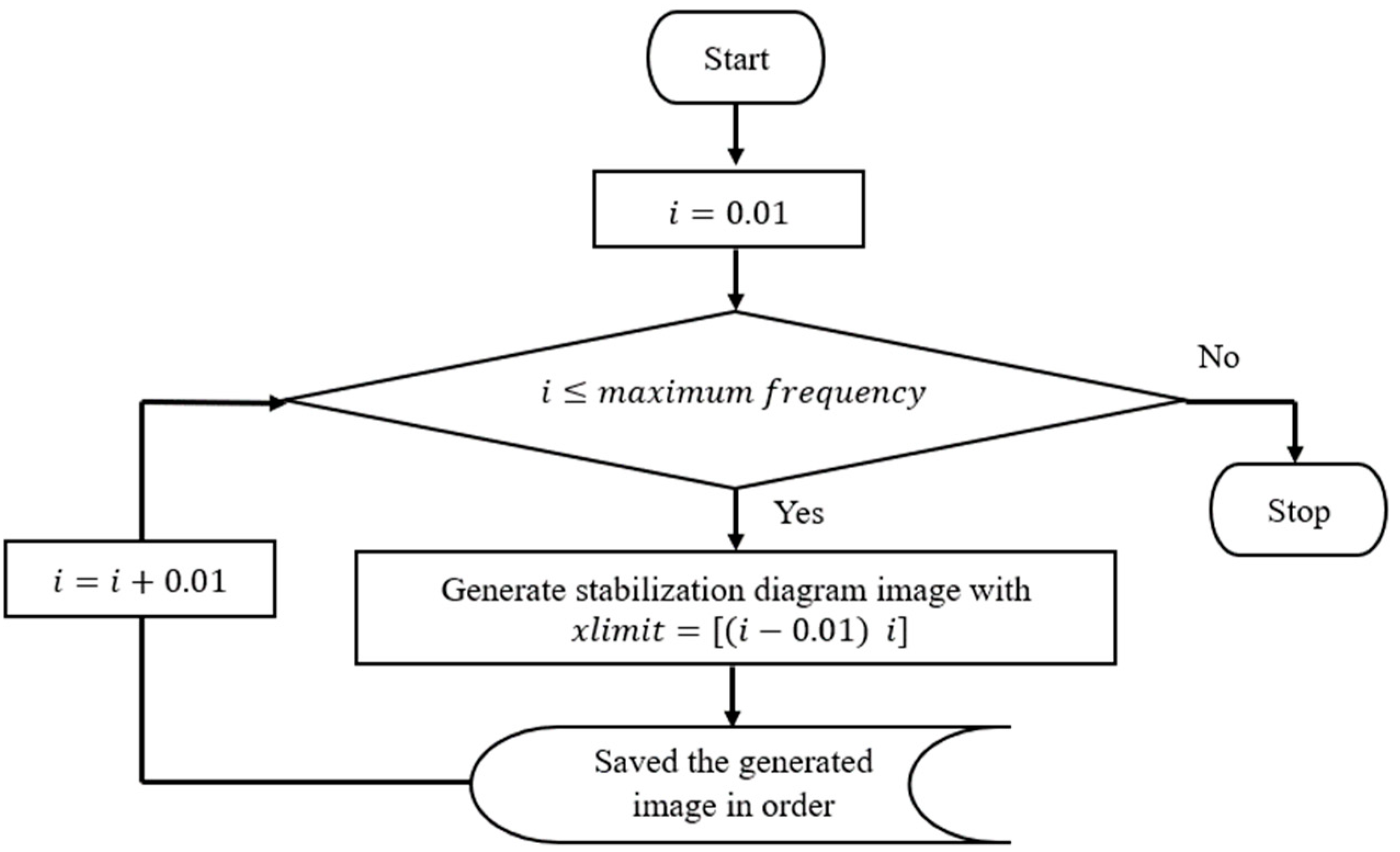
Figure 3.
Flowchart process of generated input images from a stabilization diagram with a 0.01 Hz interval frequency.
Figure 3.
Flowchart process of generated input images from a stabilization diagram with a 0.01 Hz interval frequency.
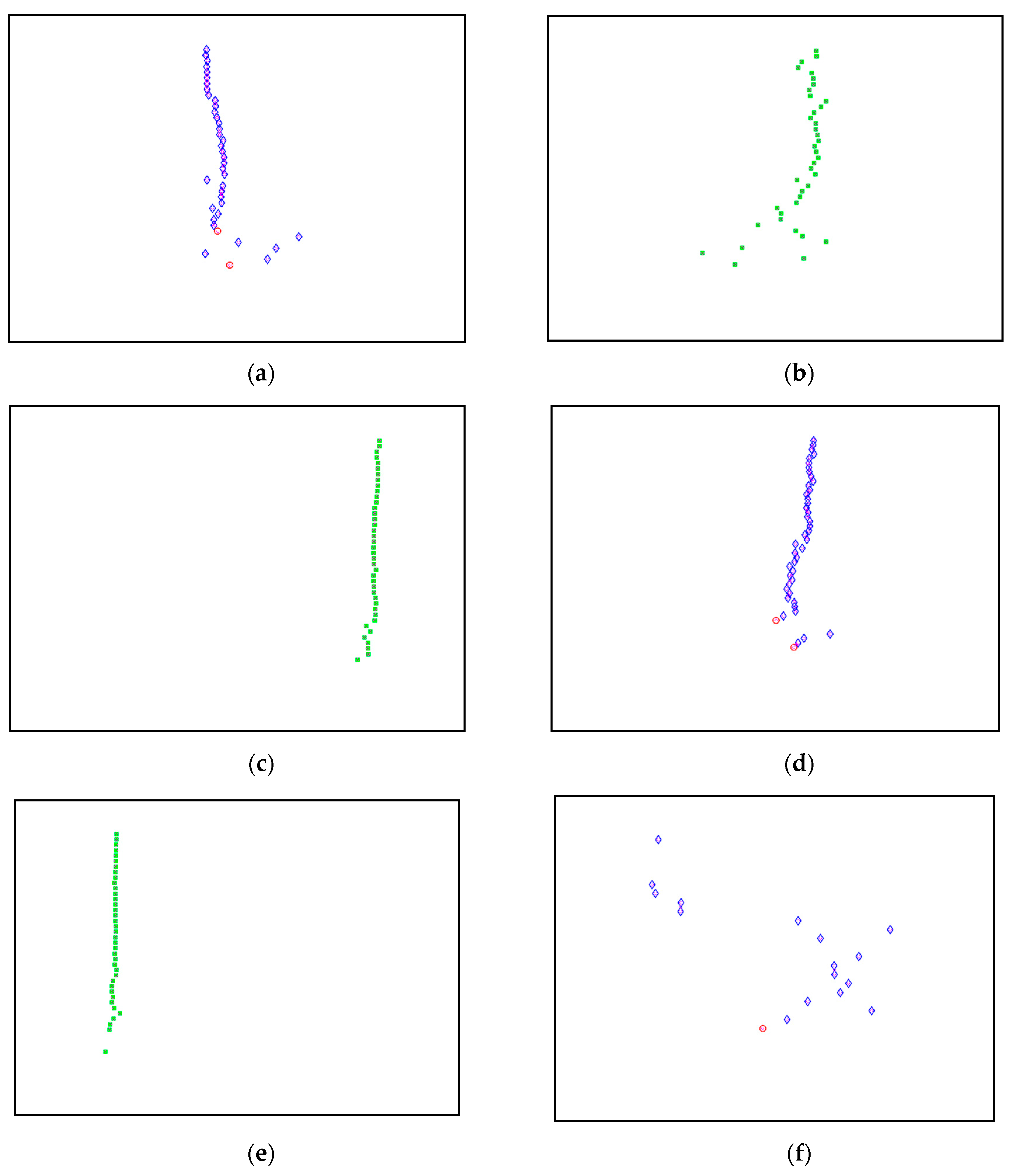
Figure 4.
Illustration of example generated input images from a stabilization diagram with a 0.1 Hz interval frequency for feature extraction for 5 Hz maximum frequency.
Figure 4.
Illustration of example generated input images from a stabilization diagram with a 0.1 Hz interval frequency for feature extraction for 5 Hz maximum frequency.
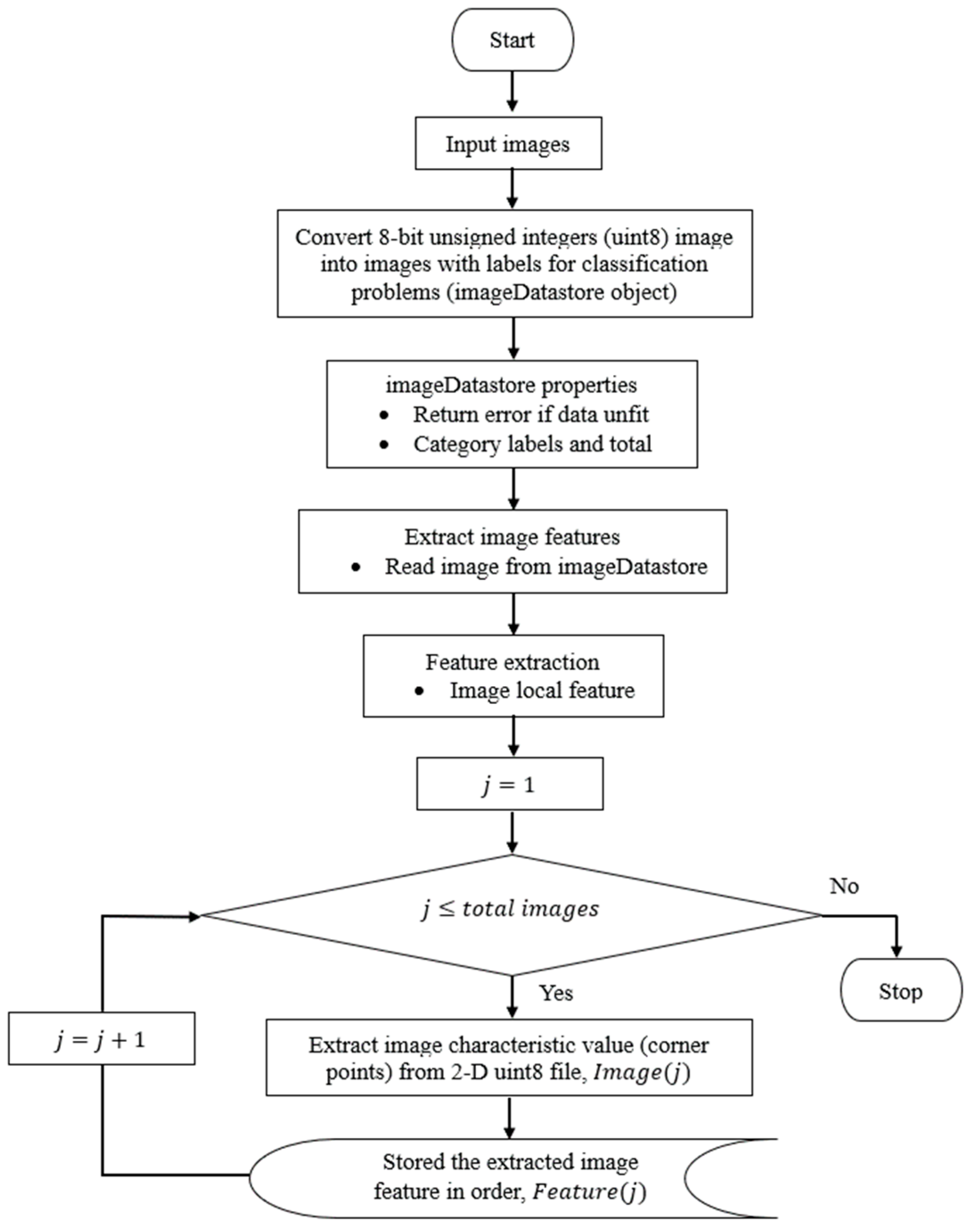
Figure 5.
Flowchart process of image feature extraction.
Figure 5.
Flowchart process of image feature extraction.
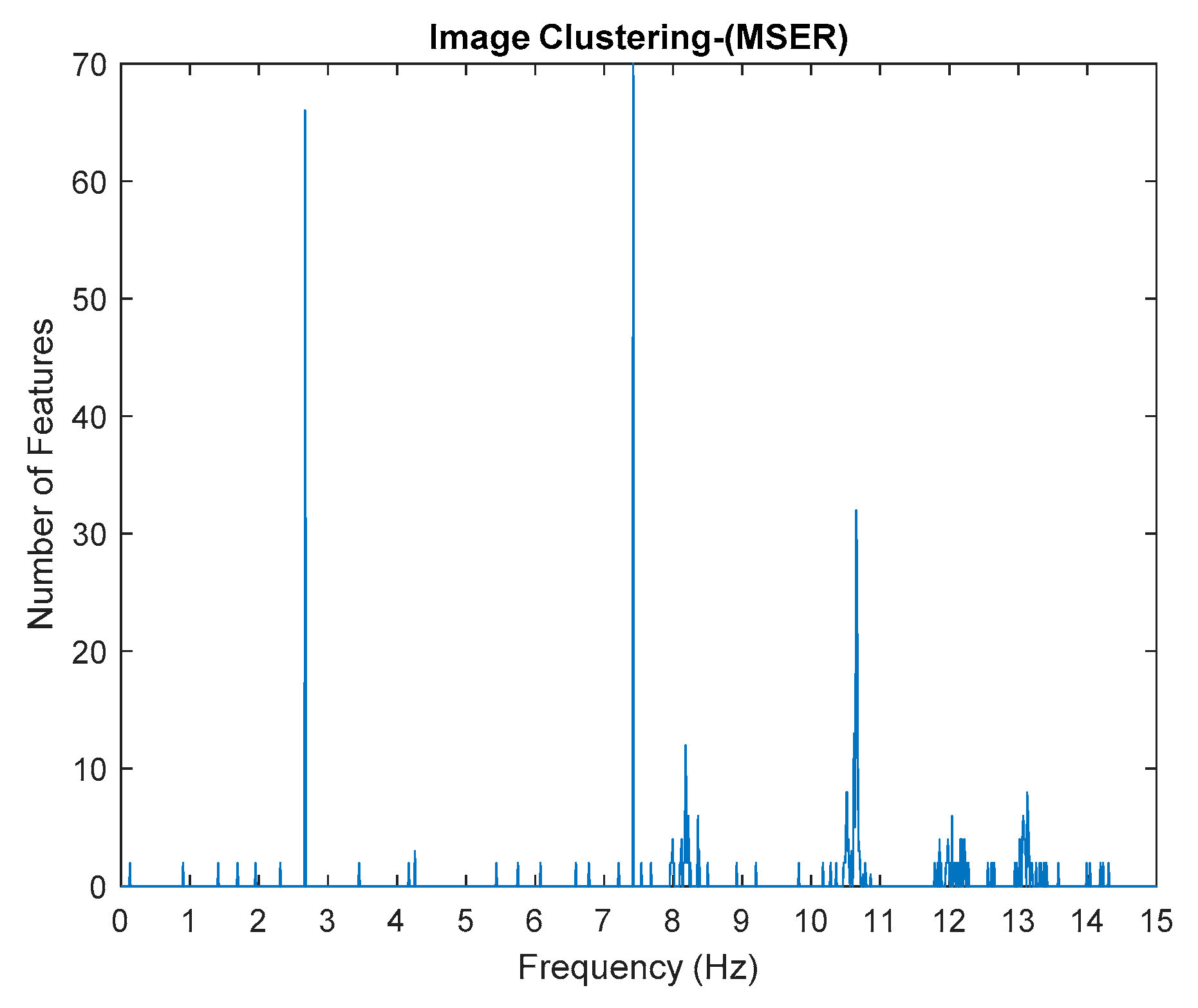
Figure 6.
Image clustering plot by using image features extraction from Maximally Stable External Regions (MSER) of the three-story frame model from numerical simulations.
Figure 6.
Image clustering plot by using image features extraction from Maximally Stable External Regions (MSER) of the three-story frame model from numerical simulations.
Figure 7.
(a–f) First, second, third, fourth, fifth and sixth physical modes respectively, of the three-story frame model from numerical simulations.
Figure 7.
(a–f) First, second, third, fourth, fifth and sixth physical modes respectively, of the three-story frame model from numerical simulations.
Figure 8.
Flowchart of shape recognition and classifier steps. RGB image refers to three hues of light that can be mixed together to create different colors image.
Figure 8.
Flowchart of shape recognition and classifier steps. RGB image refers to three hues of light that can be mixed together to create different colors image.
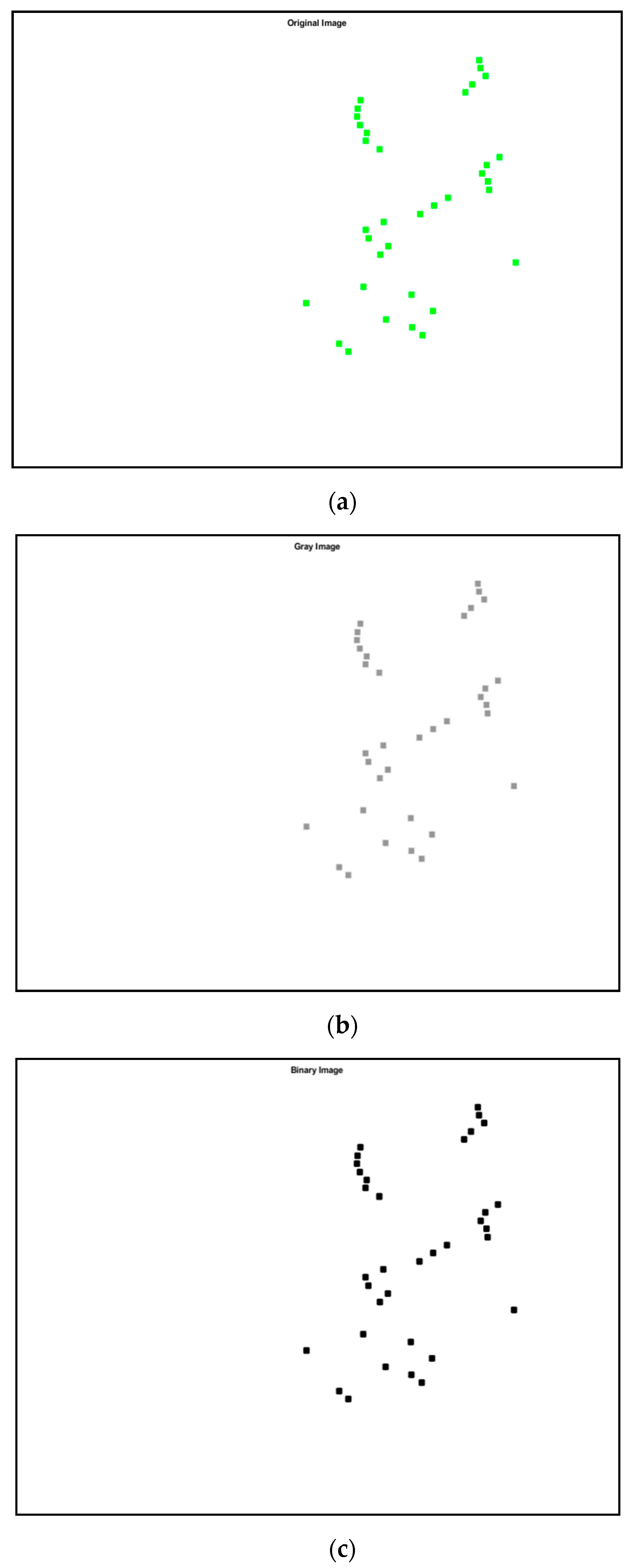
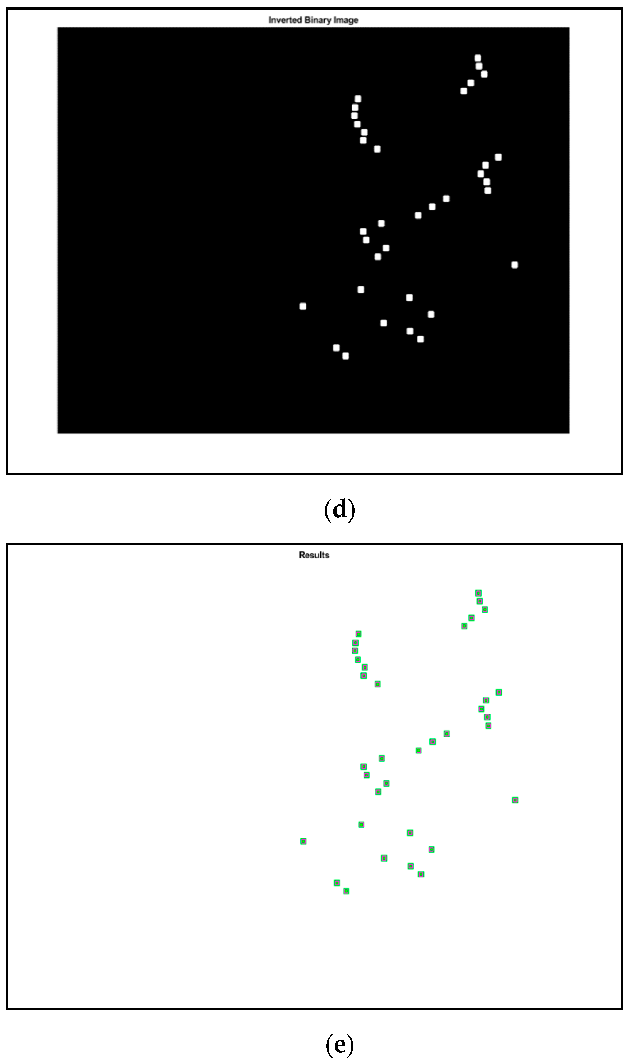
Figure 9.
Steps of the shape recognition process (a) original image, (b) grey image, (c) binary image, (d) inverted binary image and (e) results in images respectively, of the three-story frame model from numerical simulations.
Figure 9.
Steps of the shape recognition process (a) original image, (b) grey image, (c) binary image, (d) inverted binary image and (e) results in images respectively, of the three-story frame model from numerical simulations.
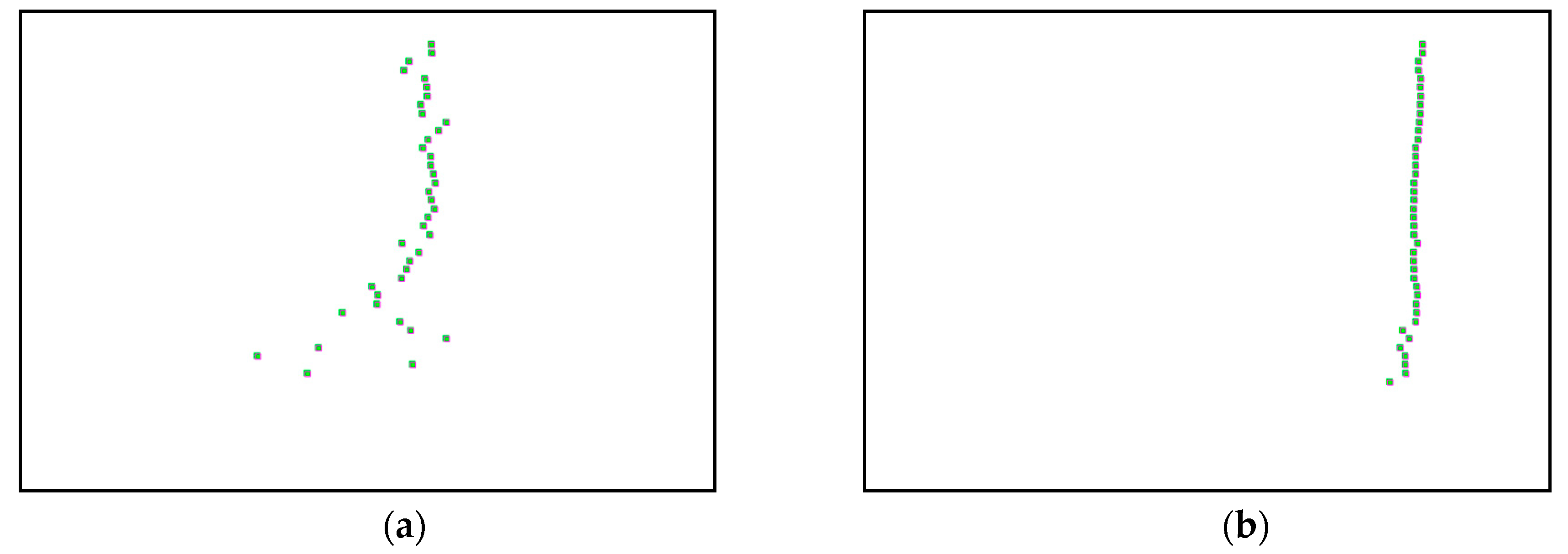
Figure 10.
(a–c) First, second and third harmonic modes respectively, detected by magenta square marker type, of the three-story frame model from numerical simulations.
Figure 10.
(a–c) First, second and third harmonic modes respectively, detected by magenta square marker type, of the three-story frame model from numerical simulations.
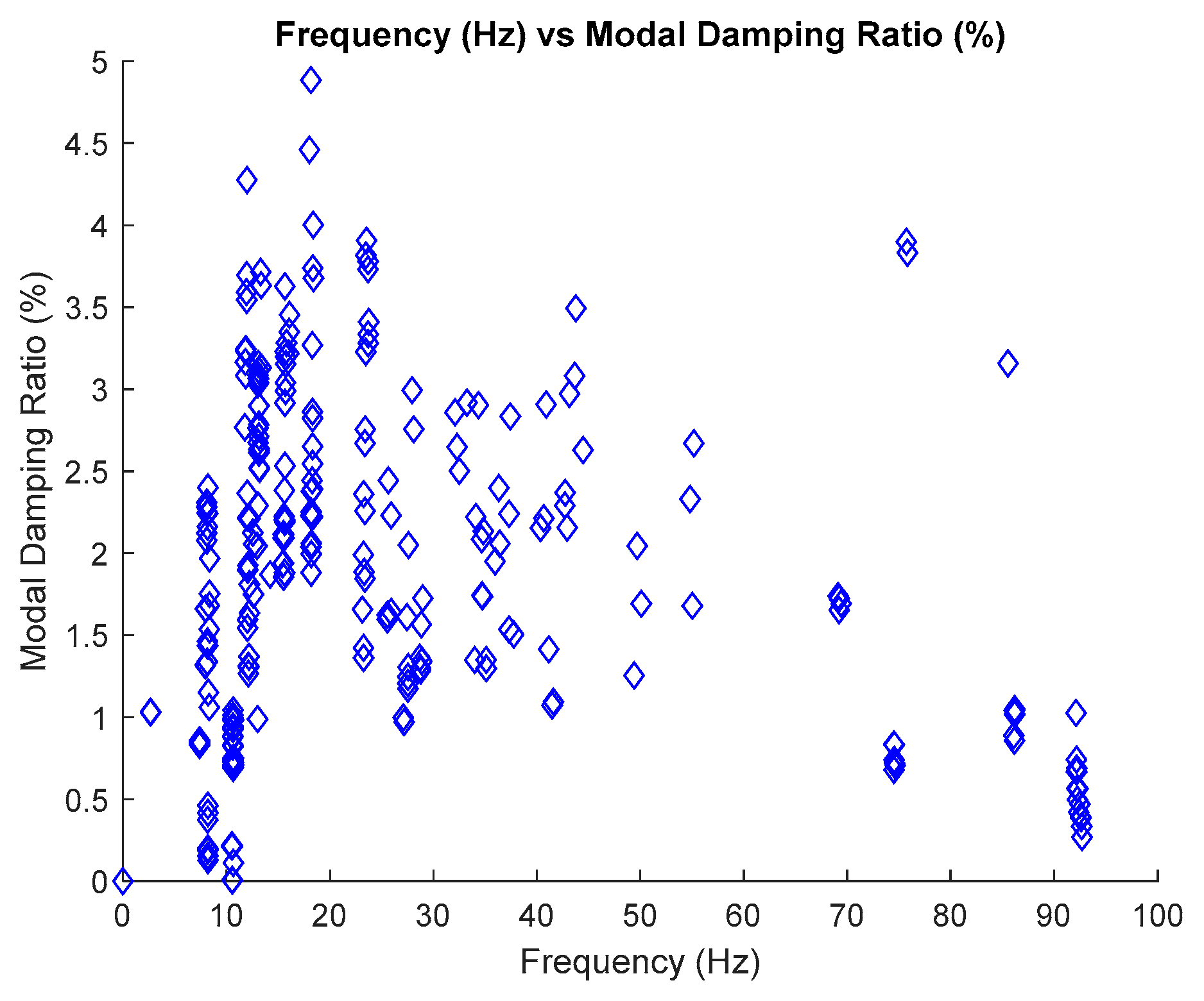
Figure 11.
Plot frequency versus modal damping ratio of the three-story frame model from numerical simulations.
Figure 11.
Plot frequency versus modal damping ratio of the three-story frame model from numerical simulations.
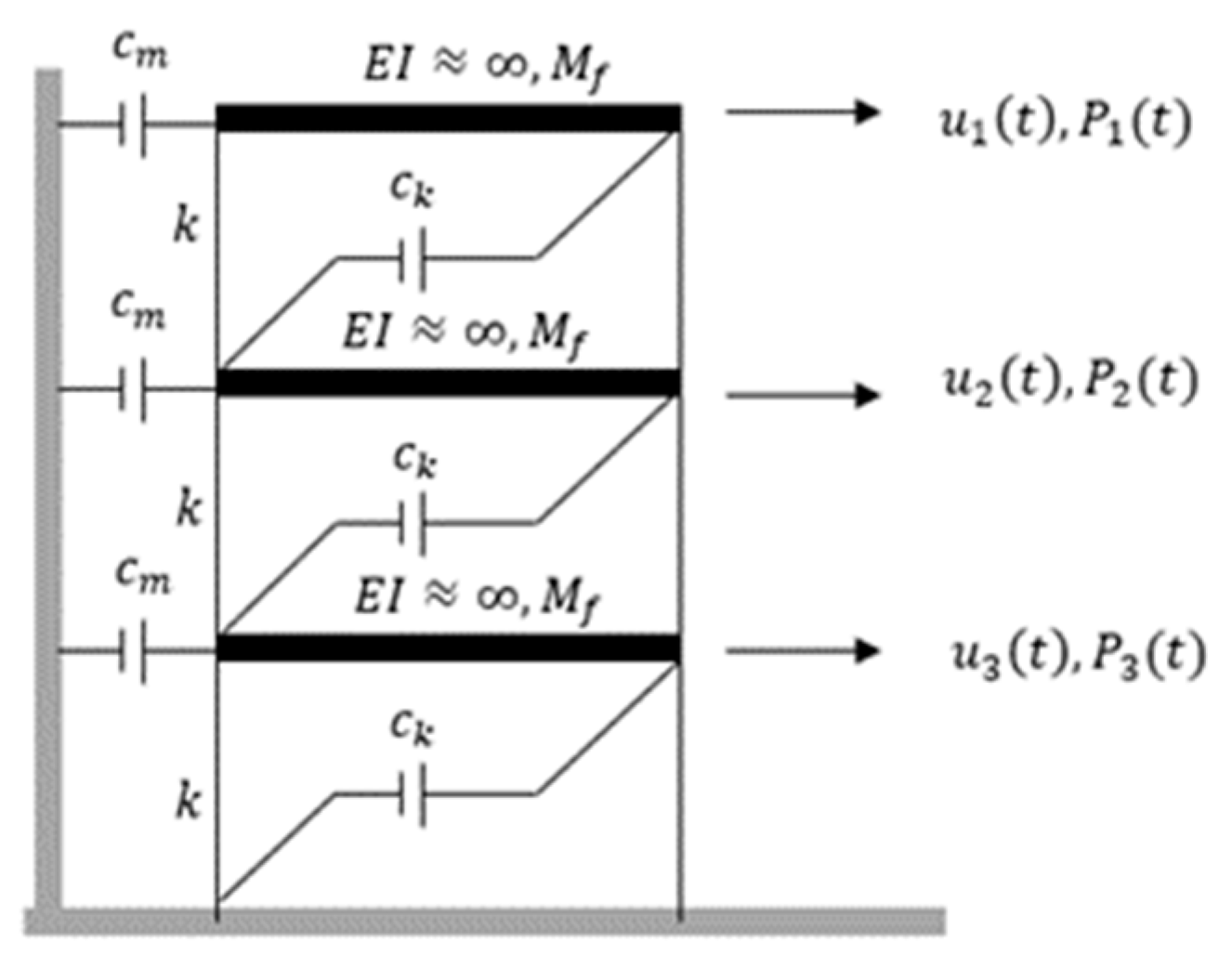
Figure 12.
Three-story frame models.
Figure 12.
Three-story frame models.
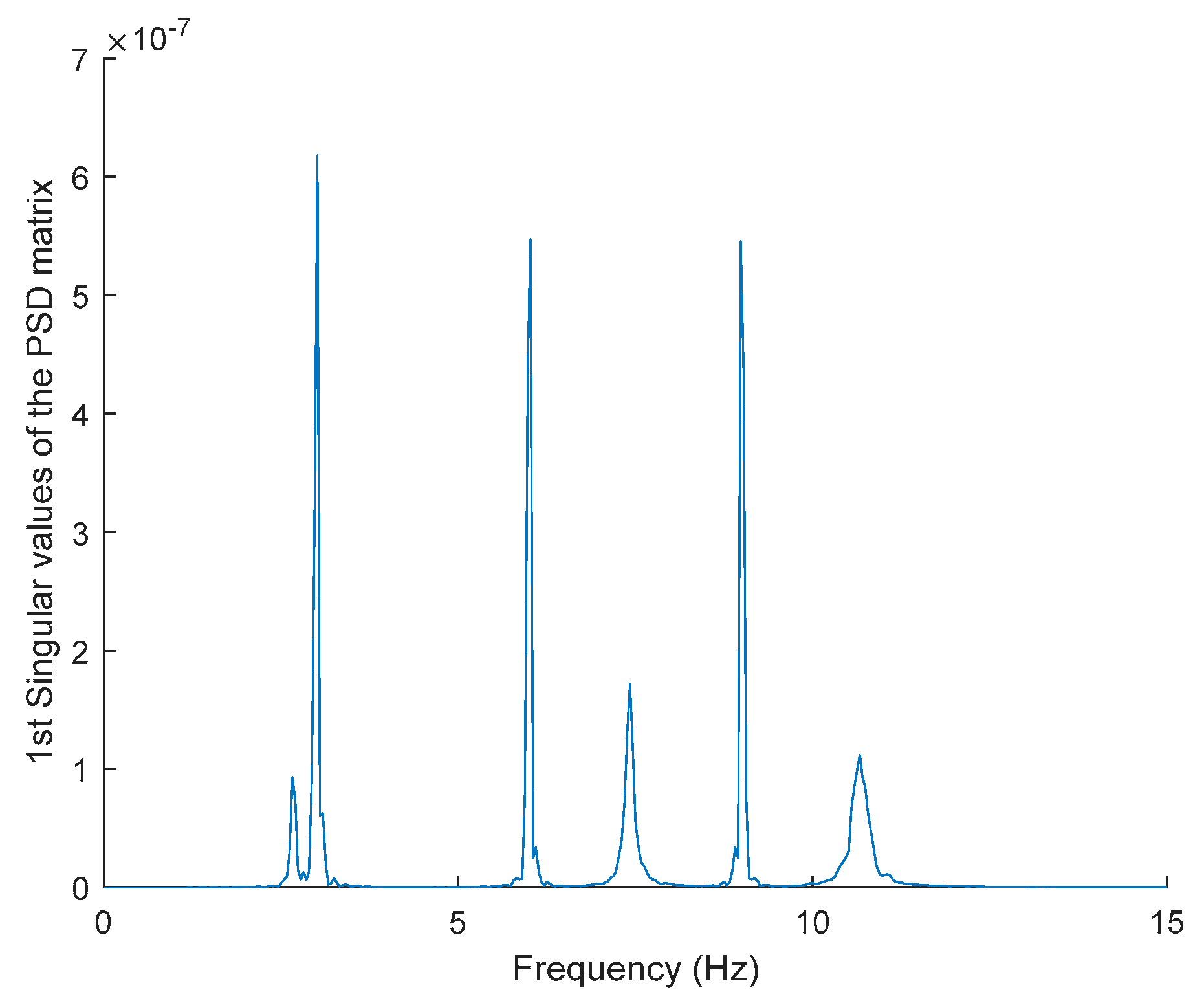
Figure 13.
The first singular values plot of the power spectral density (PSD) matrix of the original response signal.
Figure 13.
The first singular values plot of the power spectral density (PSD) matrix of the original response signal.
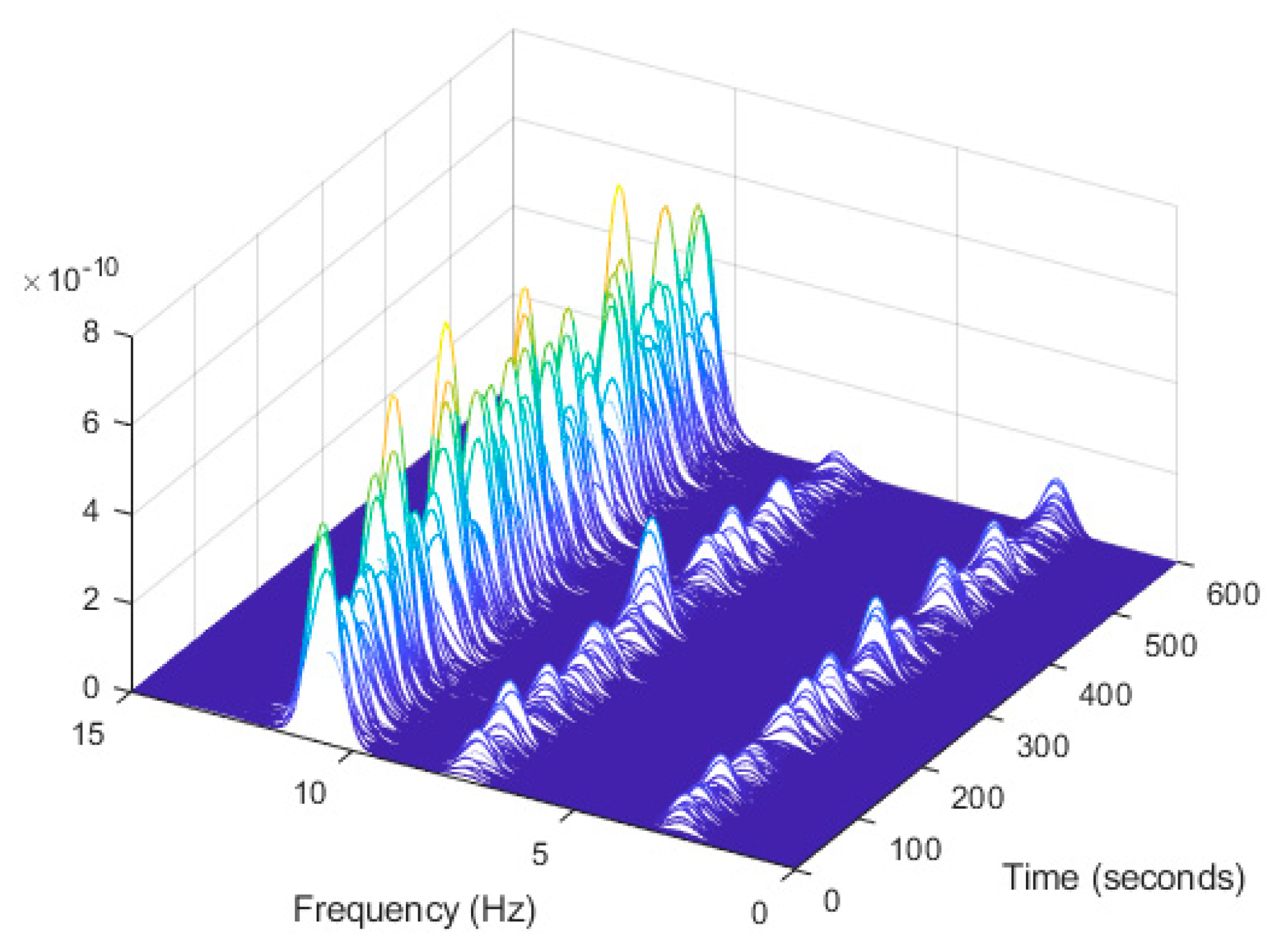
Figure 14.
Computation the spectrogram of the original response signal displayed as a waterfall plot.
Figure 14.
Computation the spectrogram of the original response signal displayed as a waterfall plot.
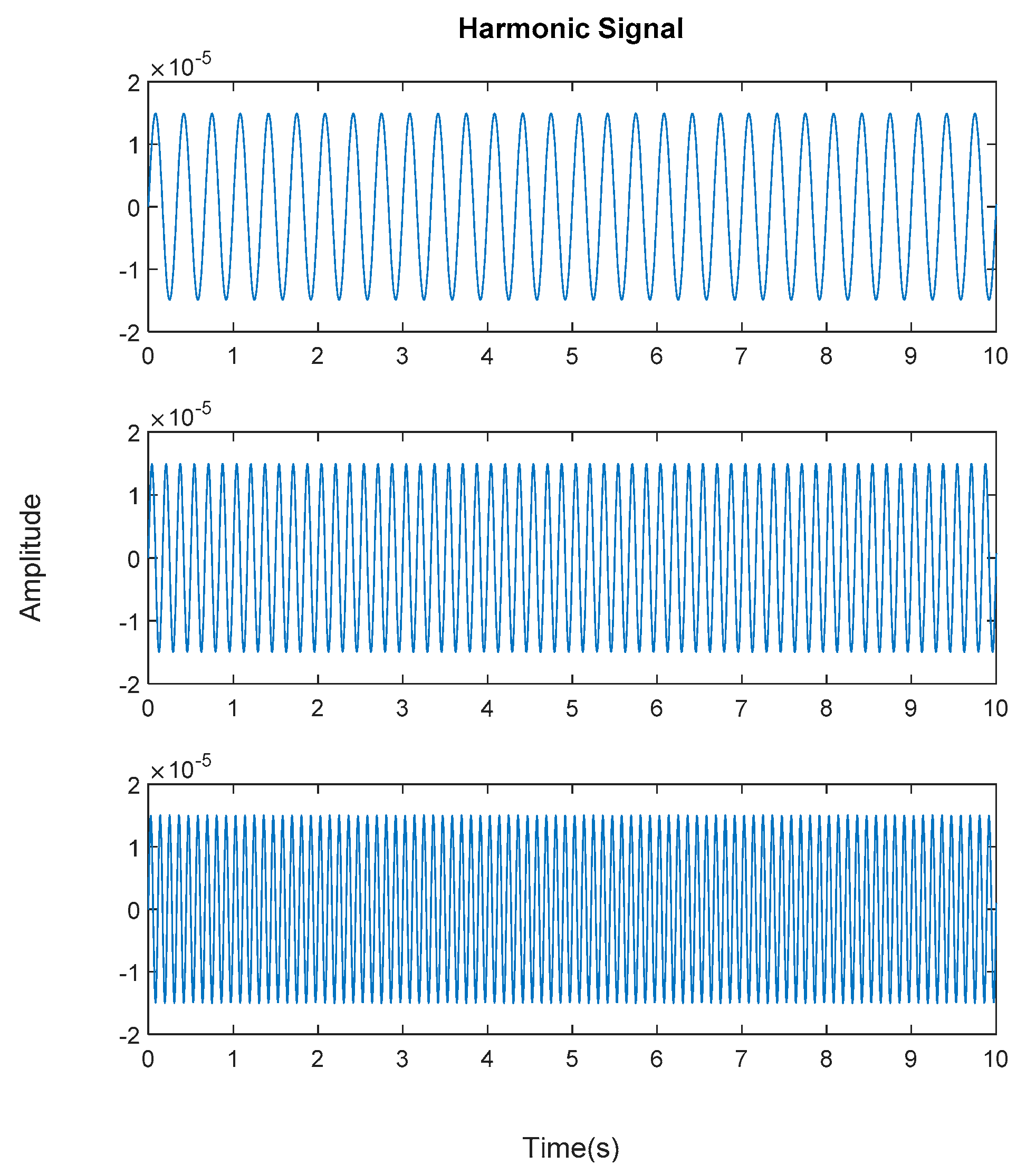
Figure 15.
Generated harmonic signal based on estimated coefficients using iterative least squares estimation. Top figure is the first harmonic component frequency; middle is second harmonic component frequency and below is the third harmonic component frequency in time domain.
Figure 15.
Generated harmonic signal based on estimated coefficients using iterative least squares estimation. Top figure is the first harmonic component frequency; middle is second harmonic component frequency and below is the third harmonic component frequency in time domain.
Figure 16.
Fast Fourier Transform (FFT) of generated harmonic signal based on estimated coefficients using iterative least squares estimation: Top figure is the first harmonic component frequency; middle is second harmonic component frequency and below is the third harmonic component frequency in frequency domain.
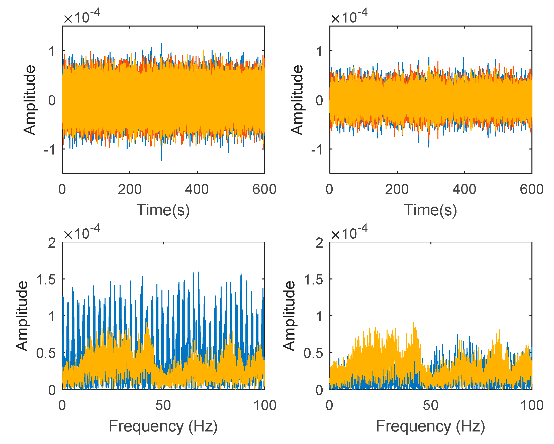
Figure 17.
Top and bottom plots are in the time domain and frequency domain respectively, while left and right side indicate signal before and after the harmonic removal process.
Figure 17.
Top and bottom plots are in the time domain and frequency domain respectively, while left and right side indicate signal before and after the harmonic removal process.
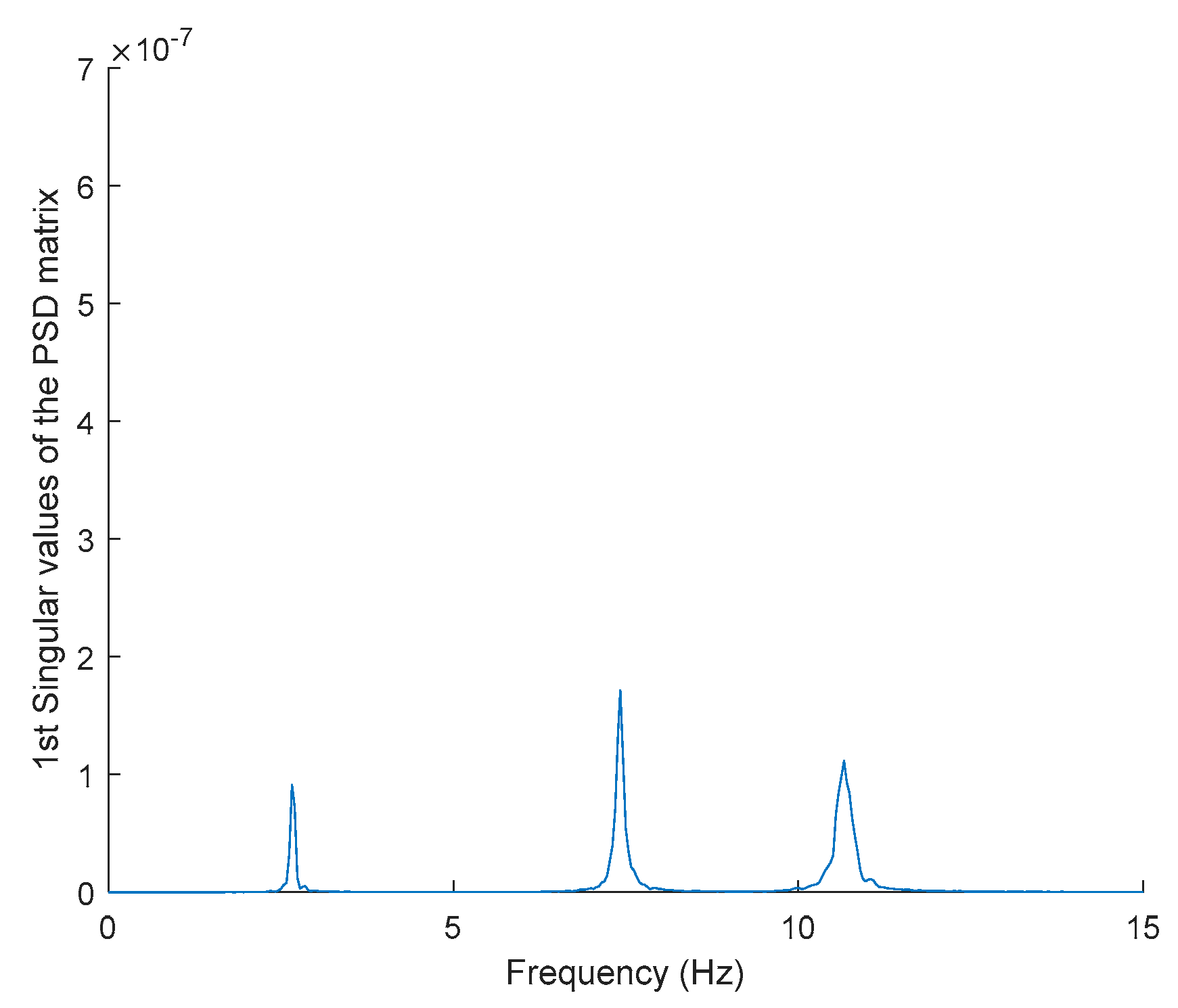
Figure 18.
The first singular values plot of the PSD matrix of the response signal after removing harmonic components.
Figure 18.
The first singular values plot of the PSD matrix of the response signal after removing harmonic components.
Figure 19.
Computation of the spectrogram of the denoising harmonic signal displayed as a waterfall plot.
Figure 19.
Computation of the spectrogram of the denoising harmonic signal displayed as a waterfall plot.
Figure 20.
Image clustering plot by using image features extraction from Maximally Stable External Regions after removing harmonic components.
Figure 20.
Image clustering plot by using image features extraction from Maximally Stable External Regions after removing harmonic components.
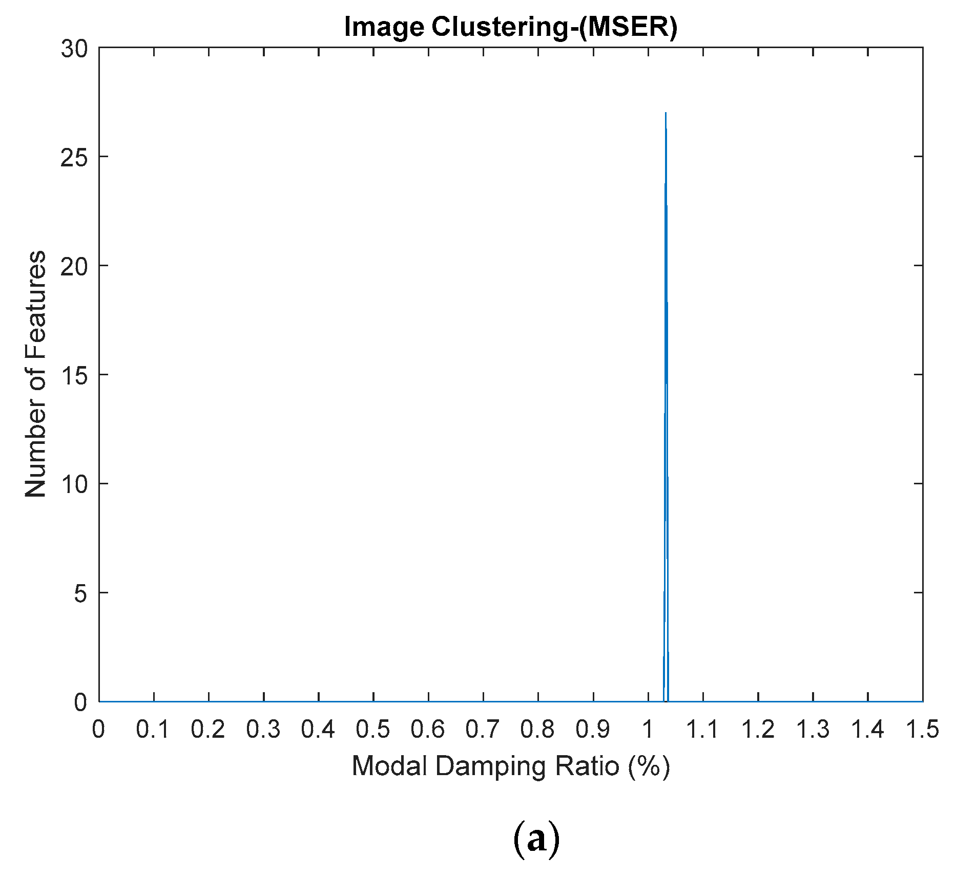
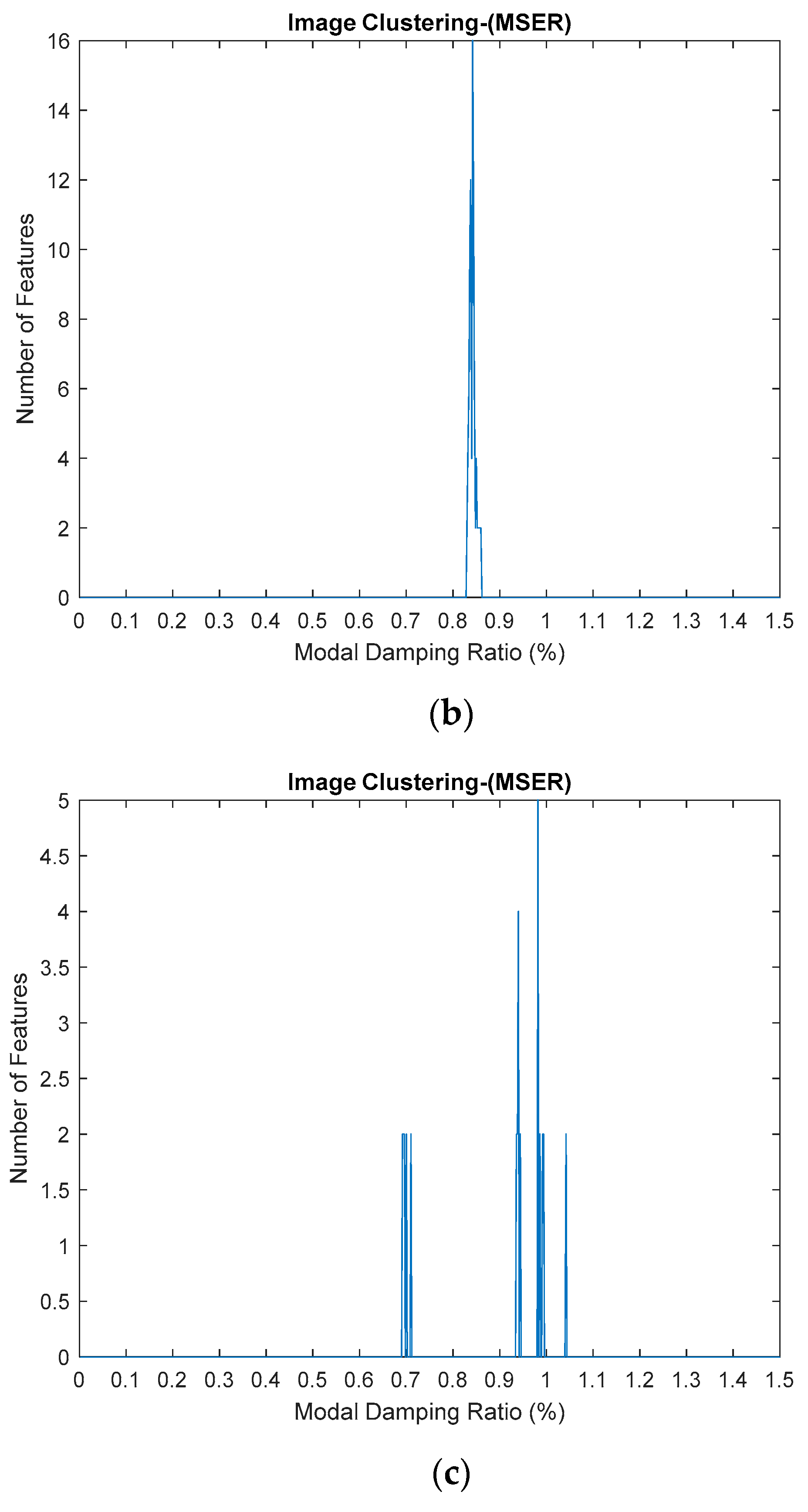
Figure 21.
(a–c) First, second and third modes for modal damping ratios respectively, of the three-story frame model from numerical simulations by using the standardized image feature, Maximally Stable External Regions (MSER) based on regions as the characteristic value.
Figure 21.
(a–c) First, second and third modes for modal damping ratios respectively, of the three-story frame model from numerical simulations by using the standardized image feature, Maximally Stable External Regions (MSER) based on regions as the characteristic value.
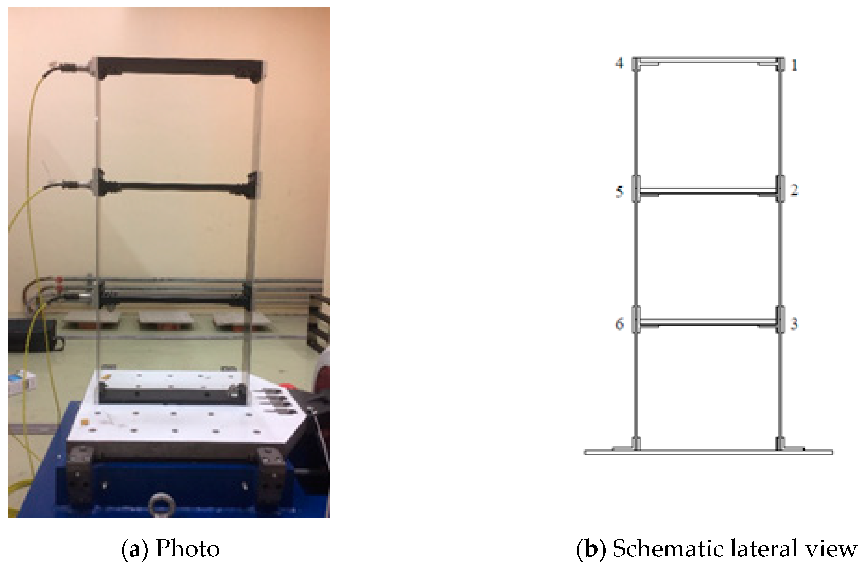
Figure 22.
General view of the metallic frame.
Figure 22.
General view of the metallic frame.
Figure 23.
Instruments set up.
Figure 23.
Instruments set up.
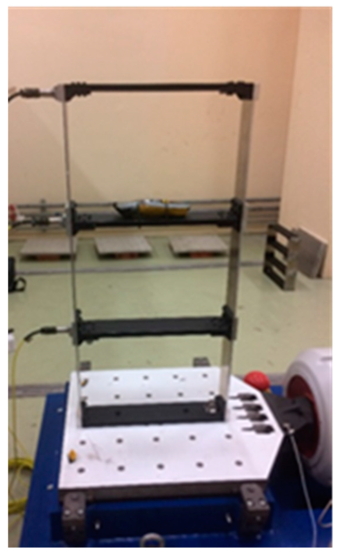
Figure 24.
Placement of rechargeable hair trimmer on the second floor.
Figure 24.
Placement of rechargeable hair trimmer on the second floor.
Figure 25.
The first singular values plot of the PSD matrix of the original response signal.
Figure 25.
The first singular values plot of the PSD matrix of the original response signal.
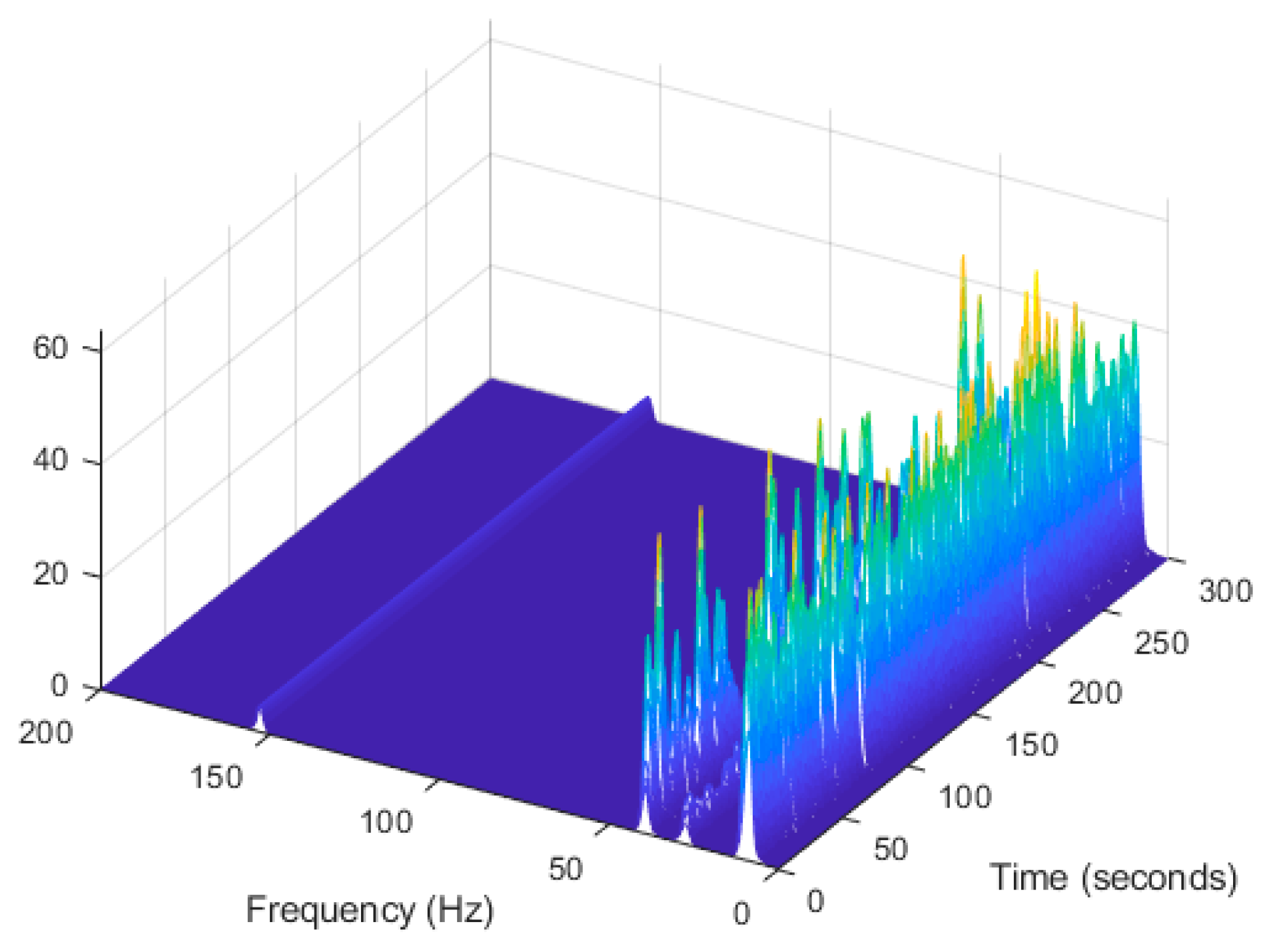
Figure 26.
Computation of the spectrogram of the original signal displayed as a waterfall plot.
Figure 26.
Computation of the spectrogram of the original signal displayed as a waterfall plot.
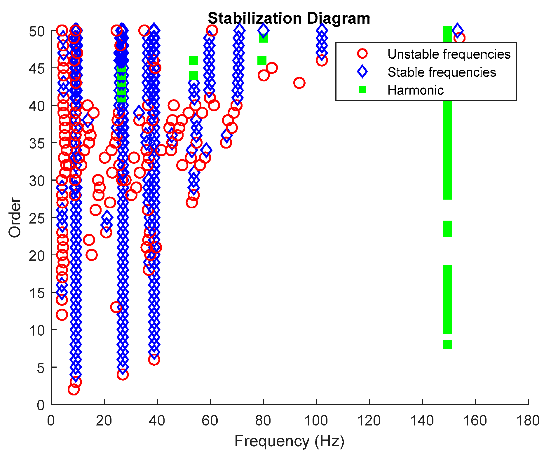
Figure 27.
Stabilization diagram plot.
Figure 27.
Stabilization diagram plot.
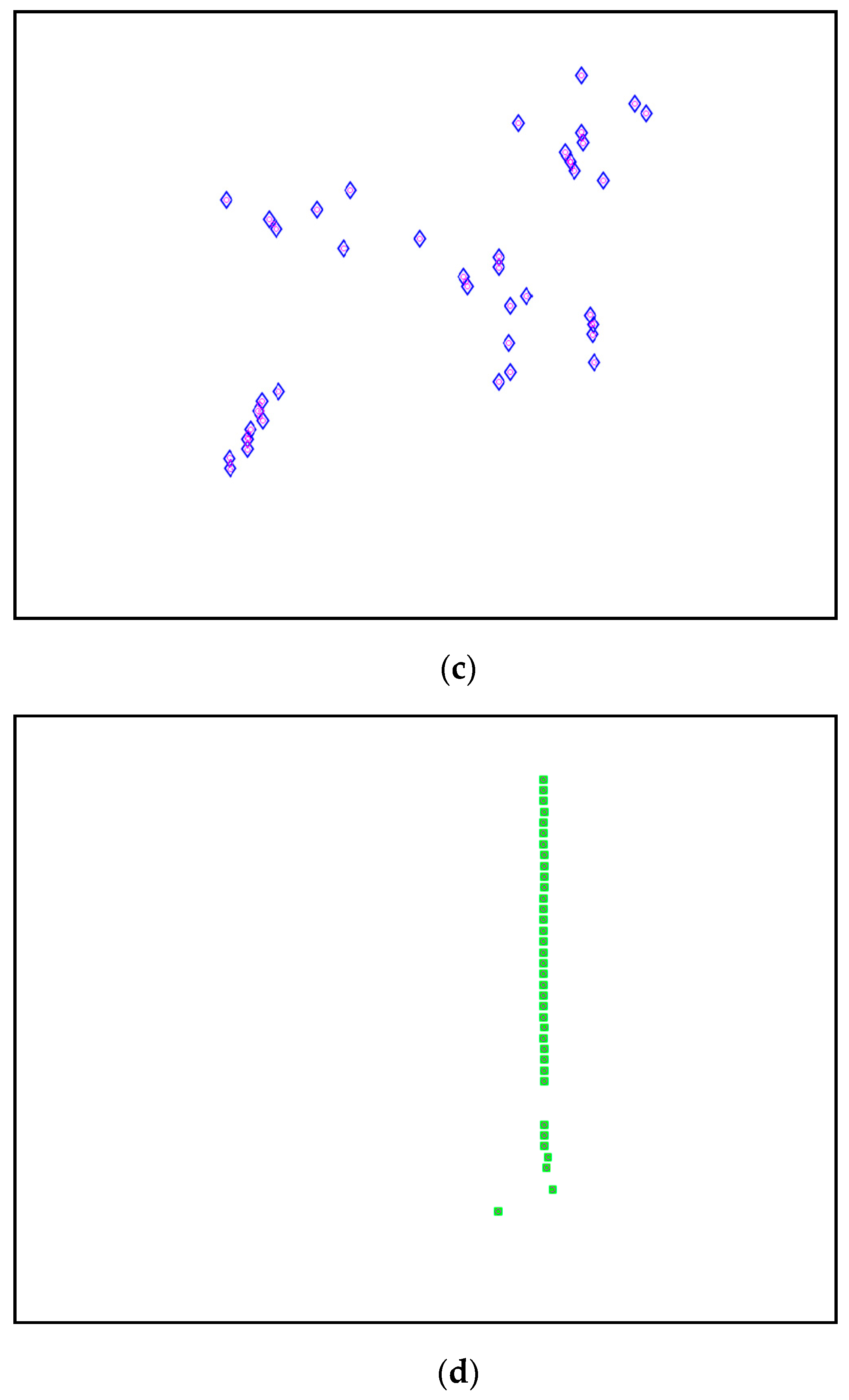
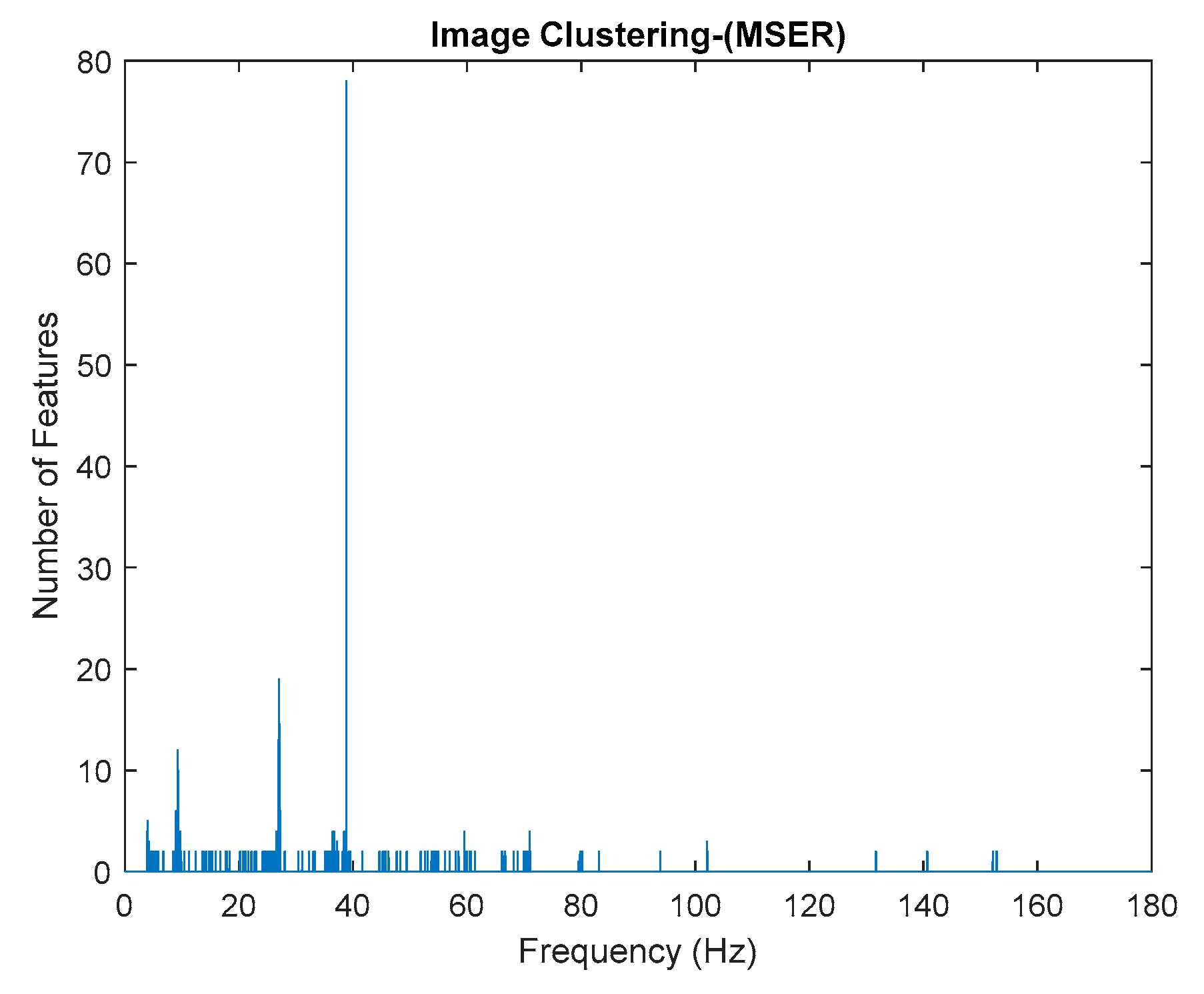
Figure 28.
Image clustering plot by using image features extraction from Maximally Stable External Regions.
Figure 28.
Image clustering plot by using image features extraction from Maximally Stable External Regions.
Figure 29.
(a–d) First, second, third and fourth physical modes, respectively.
Figure 29.
(a–d) First, second, third and fourth physical modes, respectively.
Figure 30.
Top and bottom plots are in the time domain and frequency domain respectively, while left and right side indicate signal before and after the harmonic removal process.
Figure 30.
Top and bottom plots are in the time domain and frequency domain respectively, while left and right side indicate signal before and after the harmonic removal process.
Figure 31.
The first singular values plot of the PSD matrix of the response signal after removing harmonic components.
Figure 31.
The first singular values plot of the PSD matrix of the response signal after removing harmonic components.
Figure 32.
Computation of the spectrogram of the denoising harmonic signal displayed as a waterfall plot.
Figure 32.
Computation of the spectrogram of the denoising harmonic signal displayed as a waterfall plot.
Figure 33.
Image clustering plot by using image features extraction from Maximally Stable External Regions after removing harmonic components.
Figure 33.
Image clustering plot by using image features extraction from Maximally Stable External Regions after removing harmonic components.
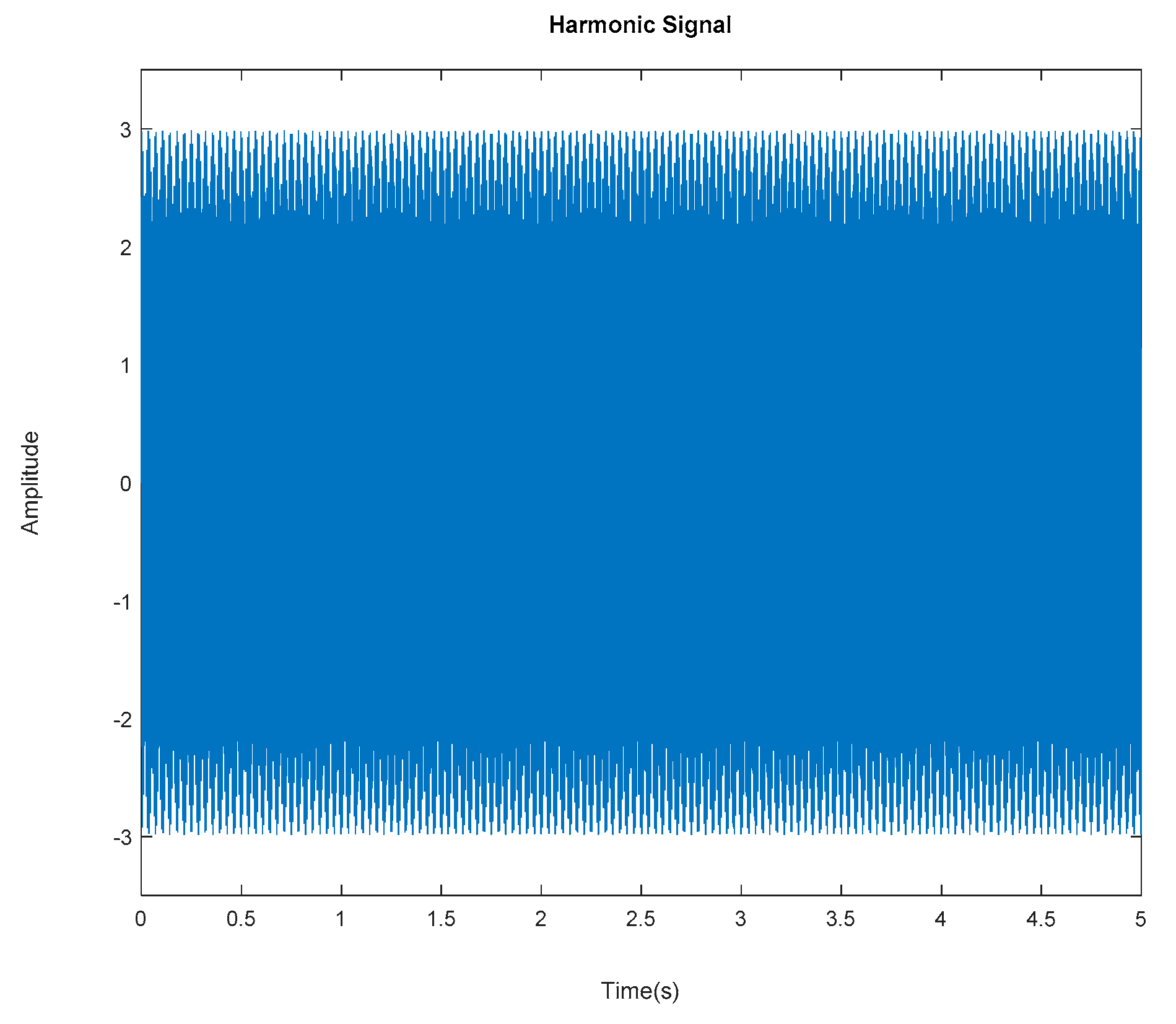
Figure 34.
Generated harmonic signal based on estimated coefficients using iterative least-squares estimation.
Figure 34.
Generated harmonic signal based on estimated coefficients using iterative least-squares estimation.
Figure 35.
FFT of the generated harmonic signal based on estimated coefficients using iterative least-squares estimation.
Figure 35.
FFT of the generated harmonic signal based on estimated coefficients using iterative least-squares estimation.
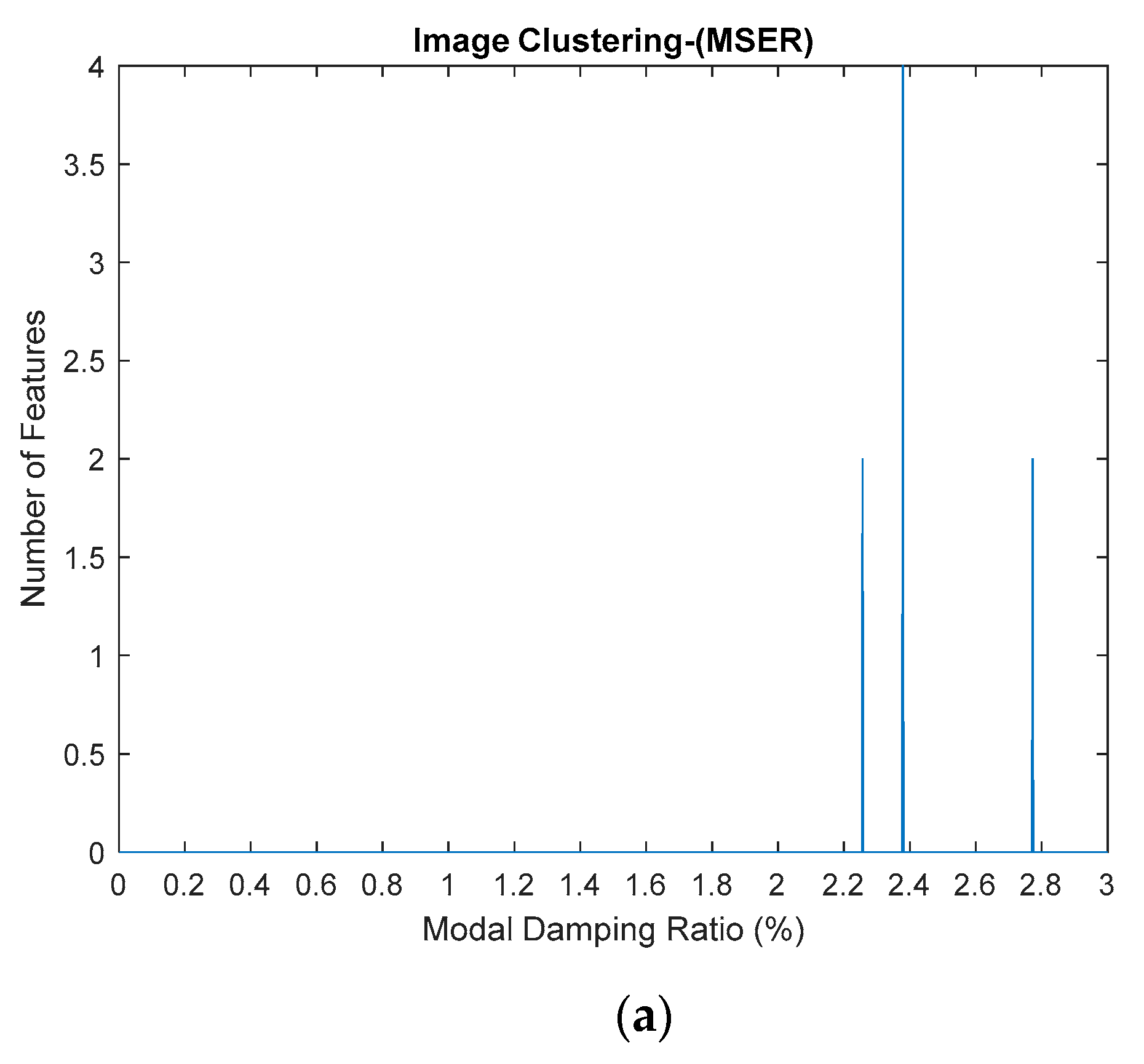
Figure 36.
Plot frequency versus modal damping ratio.
Figure 36.
Plot frequency versus modal damping ratio.
Figure 37.
(a–c) First, second and third modes for modal damping ratios, respectively.
Figure 37.
(a–c) First, second and third modes for modal damping ratios, respectively.
Table 1.
Overview of methods for identifying harmonic components and structural modes.
Table 1.
Overview of methods for identifying harmonic components and structural modes.
| Technique | Description |
|---|
| Short-Time Fourier Transform (STFT) | Short-time Fourier transform (STFT) is one of the methods of linear time-frequency domain analysis and display response in a contour plot. For structural modes, the plot will indicate thick vertical lines, while harmonic components are shown as thin vertical lines for stable conditions. |
| Singular Value Decomposition (SVD) [19] | When SVD curves are plotted, the peaks will indicate whether they are due to a harmonic component or a structural mode. If a narrow peak is shown in more than one singular value, this will indicate a harmonic excitation, while a peak of a structural mode only appears in one singular value due to the rank of the matrix. |
| Visual Mode Shapes Comparison | Operating deflection shape (ODS) will be displayed with the combination of several excited modes if the frequency of a harmonic component appears far away from a structural mode. Meanwhile, if the frequency of a harmonic component is near to structural mode, the ODS of the harmonic component will be similar to the mode shape and thus can be mistaken for being a mode shape. |
| Modal Assurance Criterion (MAC) [20] | The MAC value plays a crucial role to determine whether they are due to a harmonic component or a structural mode, which will depend on the modes being excited. The MAC value will produce a high correlation between a true mode shape and an ODS of the harmonic component, while low correlation is generated for closely spaced modes. |
| Stabilization Diagram [21,22] | A stabilization diagram can distinguish between stable, unstable and noise modes based on the specific requirements of the mode indicator and which one is respected to the set for variation between models of consecutive orders thresholds. Meanwhile, a stabilization criterion for harmonic components is identified by adjusting the valid range of damping ratios. |
| Probability Density Functions (PDFs) [23] | The significant difference in PDF distribution of a harmonic component and stochastic input can be used as a harmonic indicator. The response of stochastic input yields a PDF distribution of Gaussian-distributed bells, while the harmonic component will produce a deterministic sinusoidal response at their excitation frequency. |
| Kurtosis [16,24,25,26,27] | Kurtosis criteria have also been used to identify harmonic components and structural modes based on a significant difference in the statistical properties of PDF. The kurtosis value, γ for PDF of the sinusoidal function, is 1.5 by showing it as more “pointier”. Meanwhile, a Gaussian PDF is much wider with kurtosis value γ of 3. |
Table 2.
Specification of shape and color according to the type of poles.
Table 2.
Specification of shape and color according to the type of poles.
| Type of Poles | Type of Shape | Color |
|---|
| Stable | Diamond | Blue |
| Unstable | Circle | Red |
| Harmonic | Square | Green |
Table 3.
The adopted parameters for the three-story frame in the processing.
Table 3.
The adopted parameters for the three-story frame in the processing.
| Parameters | Three-Story Frame |
|---|
| Length of time series, (s) | 600 |
| Sampling frequency, (Hz) | 200 |
| Adopted frequency resolution, (Hz) | 0.00167 |
Table 4.
Application of fixed harmonic excitation on the three-shear frame model.
Table 4.
Application of fixed harmonic excitation on the three-shear frame model.
| Components | Harmonic Frequency (Hz) |
|---|
| 1st | 3 |
| 2nd | 6 |
| 3rd | 9 |
Table 5.
Exact modal parameter of the three-shear frame model.
Table 5.
Exact modal parameter of the three-shear frame model.
| Mode | Natural Frequency (Hz) | Modal Damping Ratio (%) |
|---|
| 1st | 2.657 | 1.00 |
| 2nd | 7.44 | 0.84 |
| 3rd | 10.76 | 1.00 |
Table 6.
Estimated dominant frequencies of the three-shear frame model.
Table 6.
Estimated dominant frequencies of the three-shear frame model.
| Components | No. of the Feature Region | No. of Figure | Identified Frequency | Nature |
|---|
| 1st | 66 | 267 | 2.67 | Structural |
| 2nd | 39 | 301 | 3.01 | Harmonic |
| 3rd | 40 | 600 | 6.00 | Harmonic |
| 4th | 69 | 742 | 7.42 | Structural |
| 5th | 40 | 901 | 9.01 | Harmonic |
| 6th | 33 | 1065 | 10.65 | Structural |
Table 7.
Estimated harmonic components of the three-shear frame model.
Table 7.
Estimated harmonic components of the three-shear frame model.
| Component | Frequency (Hz) | No. of Square Shape Recognition |
|---|
| 1st | 3.01 | 39 |
| 2nd | 6.00 | 40 |
| 3rd | 9.01 | 30 |
Table 8.
Estimated coefficient values for sinusoidal model fitting of harmonic components in the three-shear frame model.
Table 8.
Estimated coefficient values for sinusoidal model fitting of harmonic components in the three-shear frame model.
| Component | Target Coefficient Value | Estimated Coefficient Value |
|---|
| A [10−5] | B | A [10−5] | B |
|---|
| 1st | 1.500 | 3 | 1.491 | 3.01 |
| 2nd | 1.500 | 6 | 1.495 | 6.00 |
| 3rd | 1.500 | 9 | 1.505 | 9.01 |
Table 9.
Estimated damping ratios of the three-shear frame model.
Table 9.
Estimated damping ratios of the three-shear frame model.
| Mode | Number of the Feature Region | No. of Figure | Identified Damping Ratios (%) |
|---|
| 1st | 27 | 516 | 1.032 |
| 2nd | 16 | 421 | 0.842 |
| 3rd | 5 | 491 | 0.982 |
Table 10.
Comparison of estimated natural frequencies of the three-shear frame model before removing the harmonic signal.
Table 10.
Comparison of estimated natural frequencies of the three-shear frame model before removing the harmonic signal.
| Mode | Target Natural Frequency (Hz) | Natural Frequency (Hz) |
|---|
| Proposed SSI | Error (%) | Classical SSI | Error (%) | SSI-Data | Error (%) |
|---|
| 1st | 2.657 | 2.67 | 0.49 | 2.67 | 0.49 | 2.67 | 0.49 |
| 2nd | 7.445 | 7.42 | 0.34 | 7.41 | 0.47 | 7.42 | 0.34 |
| 3rd | 10.759 | 10.65 | 1.01 | 10.66 | 0.92 | 10.66 | 0.92 |
Table 11.
Comparison of estimated natural frequencies of the three-shear frame model after removing the harmonic signal.
Table 11.
Comparison of estimated natural frequencies of the three-shear frame model after removing the harmonic signal.
| Mode | Target Natural Frequency (Hz) | Natural Frequency (Hz) |
|---|
| Proposed SSI | Error (%) | Classical SSI | Error (%) | SSI-Data | Error (%) |
|---|
| 1st | 2.657 | 2.67 | 0.49 | 2.66 | 0.11 | 2.66 | 0.11 |
| 2nd | 7.445 | 7.42 | 0.34 | 7.41 | 0.47 | 7.42 | 0.34 |
| 3rd | 10.759 | 10.65 | 1.01 | 10.66 | 0.92 | 10.65 | 1.01 |
Table 12.
Estimated modal damping ratios of the three-shear frame model before removing the harmonic signal.
Table 12.
Estimated modal damping ratios of the three-shear frame model before removing the harmonic signal.
| Mode | Target Modal Damping Ratio (%) | Modal Damping Ratio (%) |
|---|
| Proposed SSI | Error (%) | Classical SSI | Error (%) | SSI-Data | Error (%) |
|---|
| 1st | 1.000 | 1.040 | 4.00 | 1.276 | 27.60 | 1.049 | 4.90 |
| 2nd | 0.841 | 0.842 | 0.12 | 0.876 | 4.16 | 0.863 | 2.62 |
| 3rd | 1.000 | 0.982 | 1.80 | 0.976 | 2.40 | 0.969 | 3.10 |
Table 13.
Comparison of estimated modal damping ratios of the three-shear frame model after removing the harmonic signal.
Table 13.
Comparison of estimated modal damping ratios of the three-shear frame model after removing the harmonic signal.
| Mode | Target Modal Damping Ratio (%) | Modal Damping Ratio (%) |
|---|
| Proposed SSI | Error (%) | Classical SSI | Error (%) | SSI-Data | Error (%) |
|---|
| 1st | 1.000 | 1.032 | 3.20 | 0.995 | 0.50 | 0.983 | 1.70 |
| 2nd | 0.841 | 0.842 | 0.12 | 0.879 | 4.52 | 0.861 | 2.38 |
| 3rd | 1.000 | 0.982 | 1.80 | 0.973 | 2.70 | 0.968 | 3.2 |
Table 14.
The adopted parameters for the steel frame in the processing.
Table 14.
The adopted parameters for the steel frame in the processing.
| Parameters | Steel Frame |
|---|
| Length of time series, (s) | 300 |
| Sampling frequency, (Hz) | 640 |
| Adopted frequency resolution, (Hz) | 0.0033 |
Table 15.
Estimated dominant frequencies of the steel frame.
Table 15.
Estimated dominant frequencies of the steel frame.
| Components | No. of the Feature Region | No. of Figure | Identified Frequency | Nature |
|---|
| 1st | 12 | 927 | 9.27 | Structural |
| 2nd | 24 | 2699 | 26.99 | Structural |
| 3rd | 71 | 3884 | 38.84 | Structural |
| 4th | 36 | 14971 | 149.71 | Harmonic |
Table 16.
Estimated harmonic components of the steel frame.
Table 16.
Estimated harmonic components of the steel frame.
| Component | Frequency (Hz) | Number of Square Shape Recognition |
|---|
| 1st | 149.71 | 36 |
Table 17.
Comparison of estimated natural frequencies of the steel frame before removing the harmonic signal.
Table 17.
Comparison of estimated natural frequencies of the steel frame before removing the harmonic signal.
| Mode | Natural Frequency (Hz) |
|---|
| Proposed SSI | Classical SSI | SSI-Data |
|---|
| 1st | 9.27 | 9.28 | 9.27 |
| 2nd | 26.99 | 26.99 | 26.99 |
| 3rd | 38.84 | 38.83 | 38.83 |
Table 18.
Comparison of estimated natural frequencies of the steel frame after removing the harmonic signal.
Table 18.
Comparison of estimated natural frequencies of the steel frame after removing the harmonic signal.
| Mode | Natural Frequency (Hz) |
|---|
| Proposed SSI | Classical SSI | SSI-Data |
|---|
| 1st | 9.27 | 9.28 | 9.27 |
| 2nd | 27.05 | 26.99 | 26.99 |
| 3rd | 38.84 | 38.83 | 38.83 |
Table 19.
Comparison of estimated modal damping ratios of the steel frame before removing the harmonic signal.
Table 19.
Comparison of estimated modal damping ratios of the steel frame before removing the harmonic signal.
| Mode | Modal Damping Ratio (%) |
|---|
| Proposed SSI | Classical SSI | SSI-Data |
|---|
| 1st | 2.380 | 2.633 | 2.468 |
| 2nd | 0.748 | 0.729 | 0.714 |
| 3rd | 0.432 | 0.427 | 0.426 |
Table 20.
Comparison of estimated modal damping ratios of the steel frame after removing the harmonic signal.
Table 20.
Comparison of estimated modal damping ratios of the steel frame after removing the harmonic signal.
| Mode | Modal Damping Ratio (%) |
|---|
| Proposed SSI | Classical SSI | SSI-Data |
|---|
| 1st | 2.378 | 2.633 | 2.468 |
| 2nd | 0.732 | 0.729 | 0.714 |
| 3rd | 0.432 | 0.427 | 0.426 |
Table 21.
Estimated damping ratios of the steel frame.
Table 21.
Estimated damping ratios of the steel frame.
| Mode | No. of the Feature Region | No. of Figure | Identified Damping Ratios (%) |
|---|
| 1st | 4 | 1189 | 2.378 |
| 2nd | 4 | 366 | 0.732 |
| 3rd | 23 | 216 | 0.432 |

 ,
, 


