Image pre-processing is an important step in the image processing pipeline. It covers a wide range of operations working on images and outputting modified images [
1], such as edge detection, contrast corrections and thresholding.
Real world images are generated by capturing a signal and reconstructing an image based on a specific model. As models are typically only able to approximate reality, uncertainty is introduced to the image reconstruction process [
2]. This means that the measured intensity of a pixel can vary depending on the underlying model resulting in a varying accuracy with respect to the original signal.
Unfortunately, image uncertainty is an often neglected aspect in image processing tasks as it is an important information about the trustworthiness of the individual image pixels [
3]. When applying image pre-processing operations to an image, not only the image changes. The image’s uncertainty is changing as well. In addition to that, the uncertainty of different pixels influences the computation of an image pre-processing algorithm. Classic image pre-processing operations do either not consider the input image’s uncertainty or miss an intuitive mode of interaction that allows users to create and review uncertainty-aware image pre-processing pipelines (see
Section 1) but a meaningful combination of both attributes is required, as
Section 2 shows.
To solve this problem, this work aims to summarize the rules for uncertainty propagation (
Section 3). This allows the transformation of the underlying uncertainty of images for arbitrary image pre-processing operations. For prominent image pre-processing operations, this paper shows how the inclusion of uncertainty information changes the computation of the image operation itself, as well as how the image operation affects the underlying image uncertainty. The presented operations can be connected, allowing the formation of a flexible uncertainty-aware image pre-processing pipeline. Furthermore, the presented approach allows an intuitive review of the composed image pre-processing pipeline utilizing different visualization techniques as shown in
Section 4.
Therefore, this work contributes:
A summary of uncertainty propagation rules
Propagation of image uncertainty throughout arbitrary image pre-processing operations
An intuitive visual system to create arbitrary image pre-processing pipelines and review the impact of the pipeline design to the image uncertainty
To show the effectiveness of the presented approach, we present scenarios where the enhanced image pre-processing methods are successfully applied (
Section 5).
Section 6 will discuss the benefits and limits of the presented approach. At last,
Section 7 summarizes this work and points out future directions.
1. Related Work
In this section, the state-of-the-art of uncertainty propagation and visualization for image pre-processing operations are discussed. Resulting from this, we are able to summarize the requirements for successful uncertainty-aware image pre-processing.
1.1. Uncertainty Propagation in Image Pre-Processing Operations
Wilson and Granlund [
4] stated that uncertainty is a fundamental result of signal processing and suggested to include this information throughout the entire image processing pipeline. This statement forms the basic motivation of the presented work. We allow a high-dimensional uncertainty quantification of the input image and transform it through arbitrary uncertainty-aware image pre-processing operations.
In his work, Pal [
5] showed, that uncertainty quantification and propagation is an important factor that affects image pre-processing operations in different applications. The work presents an uncertainty model and demonstrates how it affects the decision makers outcome. Although this is a good starting point, the presented approach shows how uncertainty information is propagated along the pre-processing pipeline and visualizes this uncertainty in each computational step.
Mencattini et al. [
6] presented a pre-processing pipeline that is adapted by considering an uncertainty quantification of the input image. Although the approach is able to adjust the results in the image pre-processing pipeline according to the underlying uncertainty quantification it is only able to consider a specific model of uncertainty. To solve this problem, the presented approach is able to handle an arbitrary amount of uncertainty measures and allows its propagation throughout an arbitrary image pre-processing pipeline.
Qiang et al. [
7] presented a method for Hough transformation that is able to consider uncertainty information of the input image. Their method showed that the results for a Hough transformation can be significantly improved. Unfortunately, they are not able to visually communicate the influence of the image uncertainty. Contrary to this, the presented approach offers a visual system that helps users to interpret the changes of the image as well as the influence of the images uncertainty.
Davis and Keller [
8] proposed a high-dimensional uncertainty model for image data and presented this space to users by using an embedded visualization of the uncertainty in the original image. Although this allows users to visualize the uncertainty of an image, it does not provide a mechanism to let users transform images and their uncertainty. Therefore, the presented approach provides users with a visual system to select arbitrary image pre-processing operations and review their results according to the underlying image uncertainty.
Yi et al. [
9] presented a method that allows the quantification and propagation of image uncertainties throughout the image vision pipeline. Although this is a good starting point for the presented approach, the system lacked a visual component where users can inspect the impact of image uncertainties for different image processing methods. Therefore, the presented approach features a visual system that allows users to build arbitrary image pre-processing pipelines and review the impact of the image’s uncertainty to the operation result and the resulting uncertainty.
1.2. Uncertainty-Aware Computer Vision
The propagation of uncertainty in computer vision is a wide spread topic [
10]. Here, approaches, such as covariance propagation [
11] or fuzzy sets [
12], can be utilized.
Hue and Pei presented an uncertainty-aware framework for road navigations [
13]. In their work, they included uncertainty about the traffic amount into the computation for a shortest path. Although this enables the expression of uncertainty of a navigation solution, the presented work is not able to visually encode the uncertainty propagation throughout their computation. In comparison to this, the presented work allows an easy to understand visualization of all computational steps and their their resulting uncertainty information.
Stachowiak et al. presented a fuzzy classifier based on an uncertainty-aware similarity measure. Although the method presents an classification of image pixels that is able to express the certainty of the computed results, the presented method does not allow a visual exploration of these results. In comparison to this, the presented method provides a visual encoding of uncertainty throughout the entire computational pipeline.
Dragiev et al. [
14] presented an uncertainty-aware approach to help an automated system in detecting grasping of humans. Here, the computation includes uncertainty-information which is utilized to refine the grasping detection. Although this is a good starting point to introduce uncertainty information into a computational workflow, the approach is not able to communicate the uncertainty that is utilized for decision making. Contrary to this, the presented approach includes refined image operations based on uncertainty information as well as an uncertainty propagation throughout the entire computational pipeline which is visually encoded.
1.3. Uncertainty-Aware Visualization of Images
Uncertainty visualization is a broad topic that was summarized by Bonneau et al. [
15].
Volume rendering [
16,
17] can be used to encode the degree of trust for different regions in the volume rendered scan. Although this can provide a suitable overview of how accurate specific image areas are, these techniques are not able to visualize multiple uncertainty criteria. Therefore, the presented technique is capable of visualizing a multi-variate uncertainty space for medical image data.
Multi-variate visualization [
18] can be accomplished for all possible kinds of data. Volume rendering [
19,
20,
21] utilizing specific transfer functions to visually encode multiple values and their similarities per grid are widely used. Although these techniques offer a suitable volume visualization for multi-variate volume datasets, they can lead to visual clutter. To solve this problem, the presented technique utilizes an iso-surface based visualization that is embedded into the original image.
Gillmann et al. presented a visualization that indicates different areas in the image that show the same uncertainty behavior [
22]. Their technique utilizes iso-lines to indicate different areas of uncertainty behavior and embeds this information in the original image. Their method shows that this allows users to easily understand the nature of the high-dimensional uncertainty space and how it is correlated to the input image. We use this work as a starting point and show how we can utilize this technique for the image processing pipeline.
The state-of-the-art analysis shows that there is clear lack of an uncertainty-aware image pre-processing mechanism that is able to visually communicate the uncertainty information throughout the computational pipeline.
2. Requirements for Uncertainty-Aware Image Pre-Processing
The state-of-the-art analysis of uncertainty-aware image pre-processing showed that there is a clear lack of uncertainty-aware image pre-processing which is assisted by an intuitive and interactive visualization. This motivates the presented work. The required subcriteria to achieve such an uncertainty-aware image pre-processing will be discussed in this section.
2.1. Uncertainty-Awareness
To achieve an uncertainty-aware image pre-processing approach, Sacha et al. [
23] defined four requirements that need to be fulfilled in order to achieve a holistic uncertainty-awareness. These are summarized below:
U1 Quantify uncertainty in each point
U2 Visualize uncertainty information
U3 Enable interactive uncertainty exploration
U4 Propagate and aggregate uncertainty
In their work, Maack et al. [
24] showed that the implementation of these principles help users to better understand the underlying dataset. As a result of this, the presented paper aims to implement the uncertainty principles to achieve an uncertainty-aware image processing.
2.2. Meaningful Visualization
In order to achieve a visual system that allows users to create and review an arbitrary image pre-processing pipeline, a meaningful visualization is required. To accomplish this, several requirements need to be fulfilled as summarized by Gillmann et al. [
25]. Namely, they are:
M1 Usability
M2 Effectiveness
M3 Correctness
M4 Intuitiveness
M5 Flexibility
In order to achieve a successful uncertainty-aware image pre-processing, both groups of requirements (C1-4, M1-5) need to be fulfilled. This forms the basic motivation for the presented work.
3. Definitions
In the following section, image definitions and the propagation rules of uncertainty will be summarized.
3.1. Image Definition
An image
I can be defined as
where
z is the number of pixels. Therefore each Pixel consists of a Position
v that describes a position in space
V. This position space can be defined as
where
for
where
. In other words,
d describes the dimensionality of the image whereas each
defines the number of voxels in each dimension. For example, an image with
pixel would mean
,
,
and
.
Depending on the image type, an image pixel can hold several values x that have to be elements from the color space with . Therefore, c is the number of scalar components that is contained in each image pixel, whereas s is the maximum value allowed in all components. A prominent example is an RGB-Image , resulting in and .
Resulting from that, a variety of functions that use images as their input:
defines a new image I with and
is the selection of all Image compartments where x and y are valid
, , , and outputting t, d, s and c as defined for images
outputting all pixels an Image that have the distance k to the pixel v
and outputting, the average pixel value and the standard deviation of all pixel values
defines the histogram of the image. This functions outputs the occurrences of a specific in the given input image
In the following subsections, we consider two-dimensional images although the mentioned definition is not restricted in its dimensionality.
3.2. Uncertainty Propagation Rules
The propagation of uncertainty is dependant on the underlying function that transforms the input values. These rules are widely used in physics. This section summarizes the most important mathematical functions and how they transform the underlying uncertainty model.
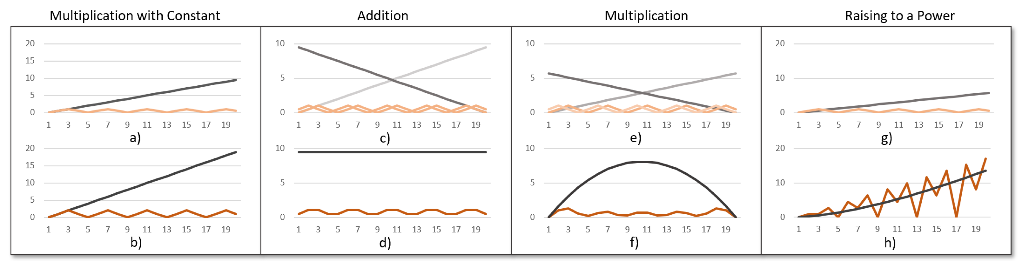
3.2.1. Multiplication by a Constant
The easiest example is the transformation of an input value through a multiplication of a constant
c. Let
, where
x is the input value and
y is the new value generated by a constant multiplication of
c. Let also
be the input uncertainty of the value
x. The transformed uncertainty
through a multiplication is defined as [
26]:
This means that the multiplication of a constant c transforms the uncertainty of a value in the same way as the value itself.
Figure 1a shows the propagation of uncertainty through a constant multiplication. The input signal (gray) is multiplied by 2. As a result, the input signal and its uncertainty are transformed as Equation (
2) shows.
Figure 1b shows the transformed signal as well as the resulting uncertainty.
3.2.2. Addition/Subtraction of Two or More Values
When adding or subtracting two or more values that are affected by uncertainty, the uncertainty propagation of the uncertainty changes. Let
be values affected by uncertainty (
). Then the combined uncertainty
resulting from addition or subtraction, with
, can be computed by [
26]:
Figure 1 shows the addition of two signals (light and dark gray) leading to one result signal. For each of the input signals, the uncertainty is shown in
Figure 1c. Using Equation (
3), the output uncertainty can be computed by using the uncertainties of the input signals leading to the result shown in
Figure 1d.
3.2.3. Multiplication/Division of Two Values
Let
x and
y be the input variables containing
and
as uncertainties. Let
or
. Computing the the uncertainty of
z can be achieved by [
26]:
Figure 1e shows an example of two input signals (light and dark gray) and their uncertainty (light and medium orange). When multiplying signals, the resulting signal and its uncertainty can be computed according to Equation (
4) as shown in
Figure 1f.
3.2.4. Raising to a Power
Let
x be a value affected by uncertainty
and let
n be a real number. When considering
, the uncertainty of
y,
, can be computed following [
27]:
Figure 1f shows a signal (gray) and its uncertainty (orange). When raising the signal to the power 1.5, the result can be seen in h) when using the formula shown in Equation (
5).
3.2.5. Arbitrary Formulas with One Variable
Let
x be a value and
, where
f is an arbitrary function allowing one variable. Then the uncertainty of
y,
, can be computed following [
28]:
3.2.6. Formulas with Multiple Variables
Let
be an arbitrary number of values and
a function using all
as input. The uncertainty of
y can be computed following [
29]:
3.2.7. Important Composed Functions
Resulting from the summarized rules of uncertainty quantification the uncertainty propagation of the functions in
Table 1 can be computed in a straightforward fashion.
The functions mentioned in
Table 1 occur in a variety of cases and are summarized for completeness. Although the summarized uncertainty propagation rules are defined for signals, the same principles can be applied to images. To accomplish this, the value contained in each image pixel is considered as one data point of a signal.
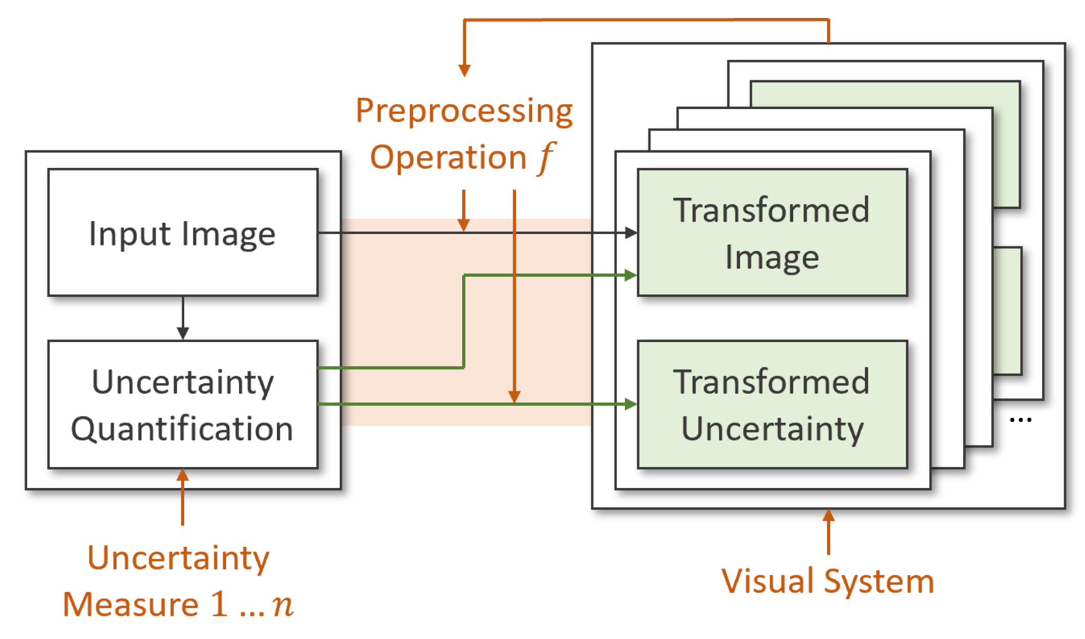
4. Methods
Based on the summarized rules of uncertainty propagation, this work aims to present an uncertainty-aware workflow for image pre-processing operations, as shown in
Figure 2. Here, a user can select arbitrary uncertainty quantification measures (see
Section 4.1) and select the visualization mode that will be utilized to display this space (see
Section 4.2). We define a set of uncertainty-aware pre-processing operations utilizing the summarized uncertainty propagation rules (see
Section 4.3). Users can connect these rules and explore the resulting uncertainty-aware pre-processing pipeline (see
Section 4.4).
4.1. Uncertainty Quantification of Input Images
Unfortunately, the term uncertainty has no unique definition. Instead, there exist a wide range of uncertainty measures that can be utilized to quantify the uncertainty of an input image [
30]. In the presented system, we allow users to select an arbitrary set of uncertainty measures and allow the transformation of uncertainty for each of those measures.
In this work, we allow users to choose an arbitrary subset from the following uncertainty measures: Acutance [
31], Contrast Stretch [
32], Gaussian Noise [
33], Brightness [
34], Local Contrast [
35], Local Range [
36] and Salt and Pepper Noise [
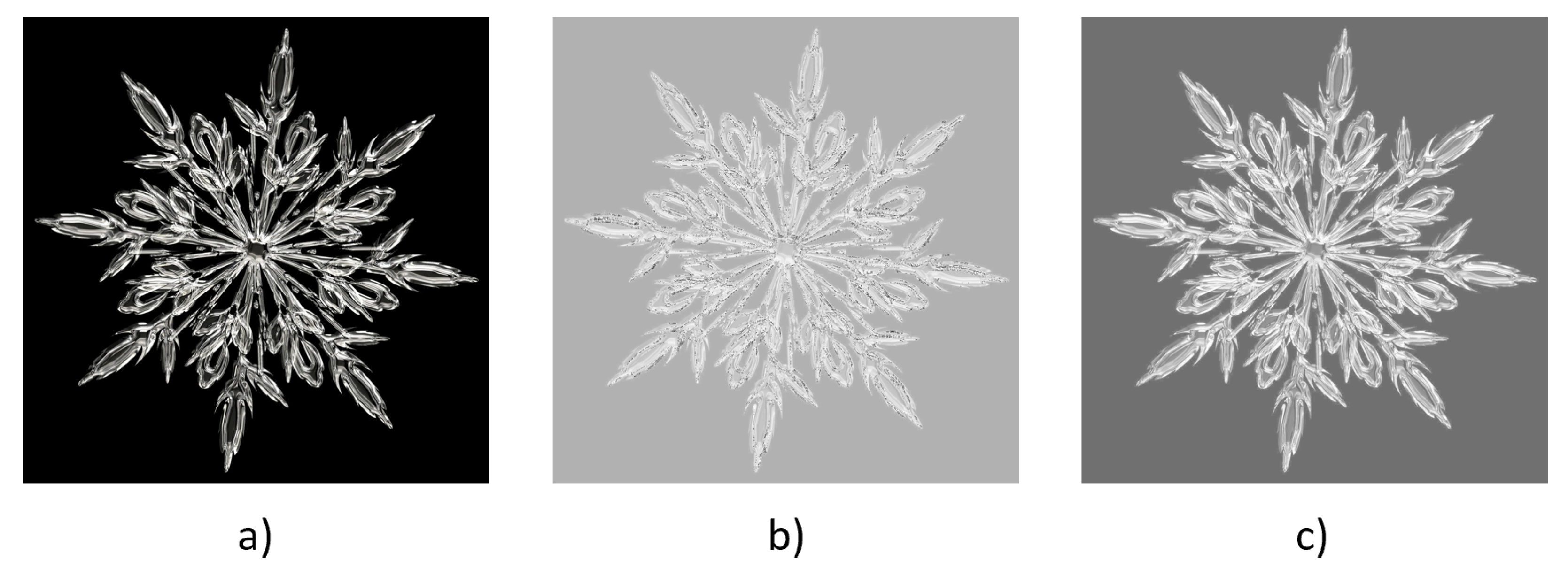
37]. An example output for all measures can be found in
Figure 3. Depending on the input dataset, users are interested in different uncertainty quantification approaches. The presented system allows users to select arbitrary uncertainty measures. The framwork then describes how these specific uncertainty measures propage through the pipleline of pre-processing algorithms.
In addition, the system allows to introduce novel uncertainty measures if users so desire. This results in a high-dimensional uncertainty space where each voxel has a vector attached describing the output of all uncertainty measures for this voxel. Furthermore, image data already containing uncertainty quantifications can be utilized in the presented system as well.
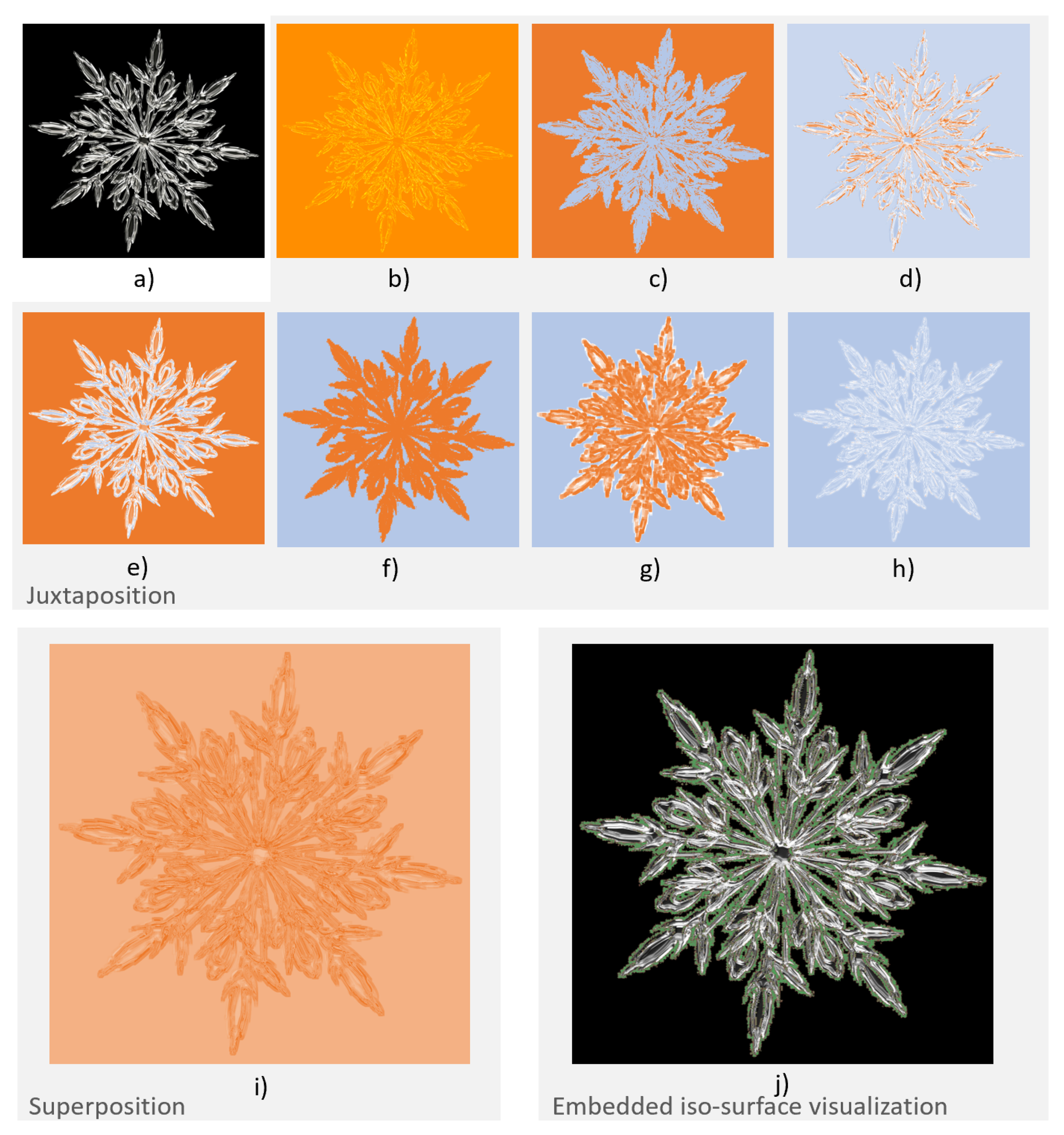
4.2. Visualization of Images and Their Uncertainty
As shown in
Section 4.1, users are enabled to select an arbitrary number of uncertainty measures to achieve an uncertainty quantification of the input image. Although this allows a holistic classification of the input images uncertainty, it also raises some issues. One problem is the review of multiple uncertainty dimensions. This is not a trivial task and can be accomplished by different techniques. In the presented methodology, we allow three different types of reviewing for each computational step in the user defined pipeline:
Juxtaposition of all uncertainty dimensions
Superposition of all uncertainty dimensions
Embedded iso-surface visualization of all uncertainty dimensions.
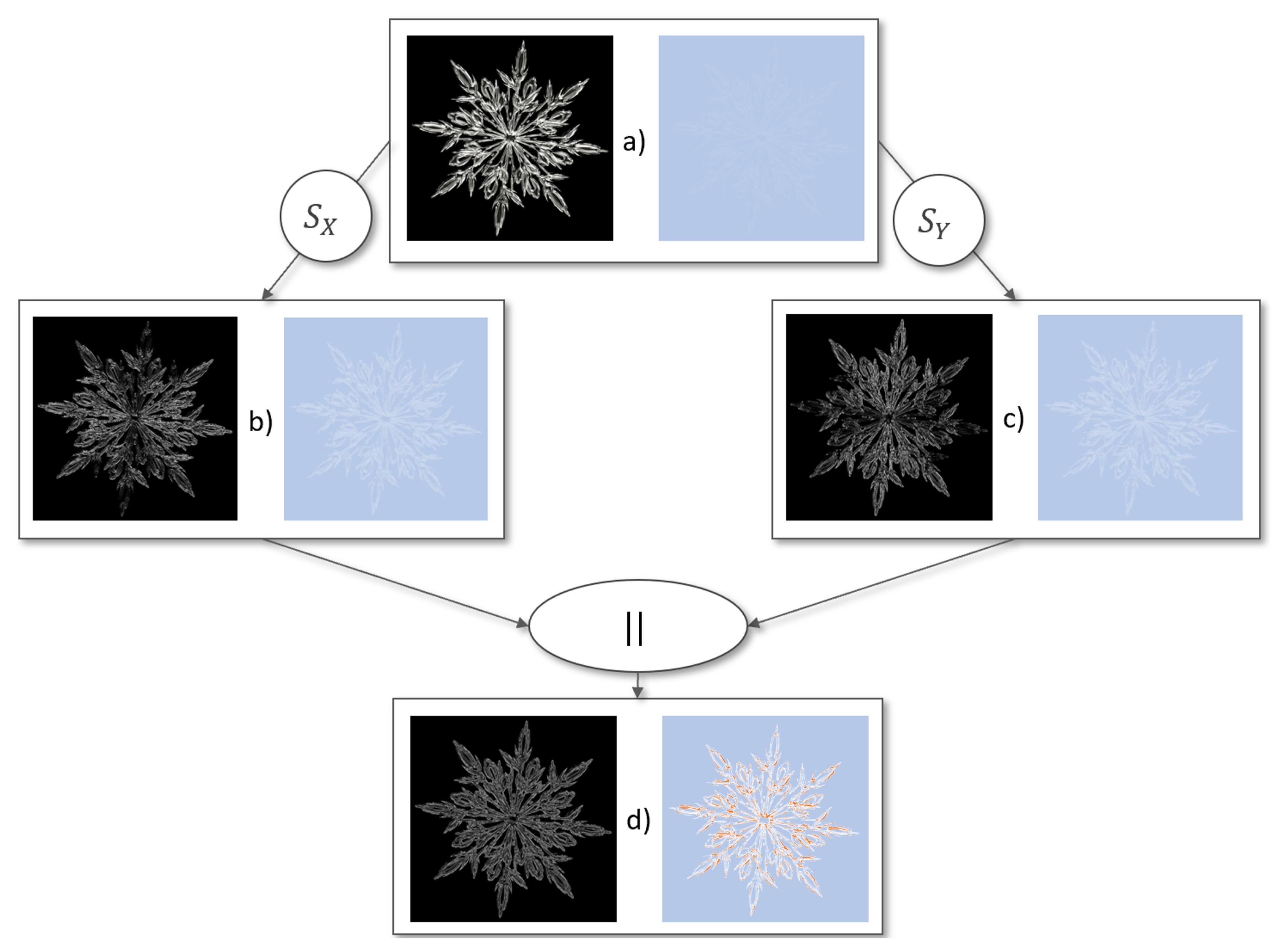
Figure 3 shows the three different visualization strategies that are available in the presented technique. They are all based on the input image).
Figure 3b–h show the result for a juxtaposition visualization of the uncertainty space. The advantage is, that all user selected uncertainty measures can be reviewed at the same time showing their exact uncertainty measures. On the other hand, the disadvantage arises as juxtaposition visualizations are very time consuming and it can be hard to compare specific uncertainty measures at defined positions.
This problem can be solved by using a superposition visualization of all chosen uncertainty measures.
Figure 3i shows the result of the superposition visualization when interpreting all chosen uncertainty measures as one dimension and computing the length of each uncertainty vector for each pixel. Other computations, such as finding the maximum of all uncertainty values or the average, can be computed as well. Although this allows the visualization of all uncertainty dimensions in one image, users are no longer able to review the composition of the individual uncertainty measures.
For both, juxtaposition and superposition, the visualizations are not able to make a direct connection to the input image. A method trying to solve this problem was presented by Gillmann et al. [
22] is utilized. Their technique utilizes iso-lines to indicate different areas of uncertainty behavior and embeds this information in the original image as shown in
Figure 3j. Their method shows that this allows user to easily understand the nature of the high-dimensional uncertainty space and how it is correlated to the input image. It is directly embedded into the original image and shows users when the underlying image uncertainty is significantly changing by utilizing iso-surfaces. When users are interested in specific uncertainty value compositions, they are enabled to select image pixels. The selected uncertainty values are then shown in a parallel coordinate plot. Although the method is able to show changes in the uncertainty of an image and emphasize specific values when requested by the users, the spatial distribution of the selected uncertainty value is lost in this visualization.
As can be seen, none of the presented visualizations is able to capture all details of the underlying uncertainty quantification. Depending on the purpose the visualization needs to fulfill, users can choose from the described visualization types to gain insights in the uncertainty of the input image as well as the uncertainty in each step of the user defined pre-processing pipeline.
4.3. Pre-Processing Steps Under Uncertainty
Based on the uncertainty propagation rules defined in
Section 3, this section shows how prominent image pre-processing techniques, such as stencils, data restoration and reduction, and convolution kernels influence the uncertainty of an input image.
4.3.1. Thresholding
Thresholding is an important image preprocessing operation that allows to select specific pixels in an image according to a selected intensity value [
38]. Without taking uncertainty information into account, the thresholding is defined as:
Instead of obtaining a hard decision on wether a value is bigger or smaller than the selected threshold, the uncertainty-aware thresholding can be defined as:
As the value T, that is utilized for thresholding can be affected by uncertainty as well, this uncertainty is also taken into the computation of the tresholding. This means that in the case of a low uncertainty for the input value and the thresold the result is close to 1 if . On the other hand, if both uncertainties are high, the result is set to 0. Instead of utilizing a global value T, the input can additionally be an entire image leading to a direct comparison of each image pixel of these input images.
The uncertainty of the resulting image can be quantified as follows:
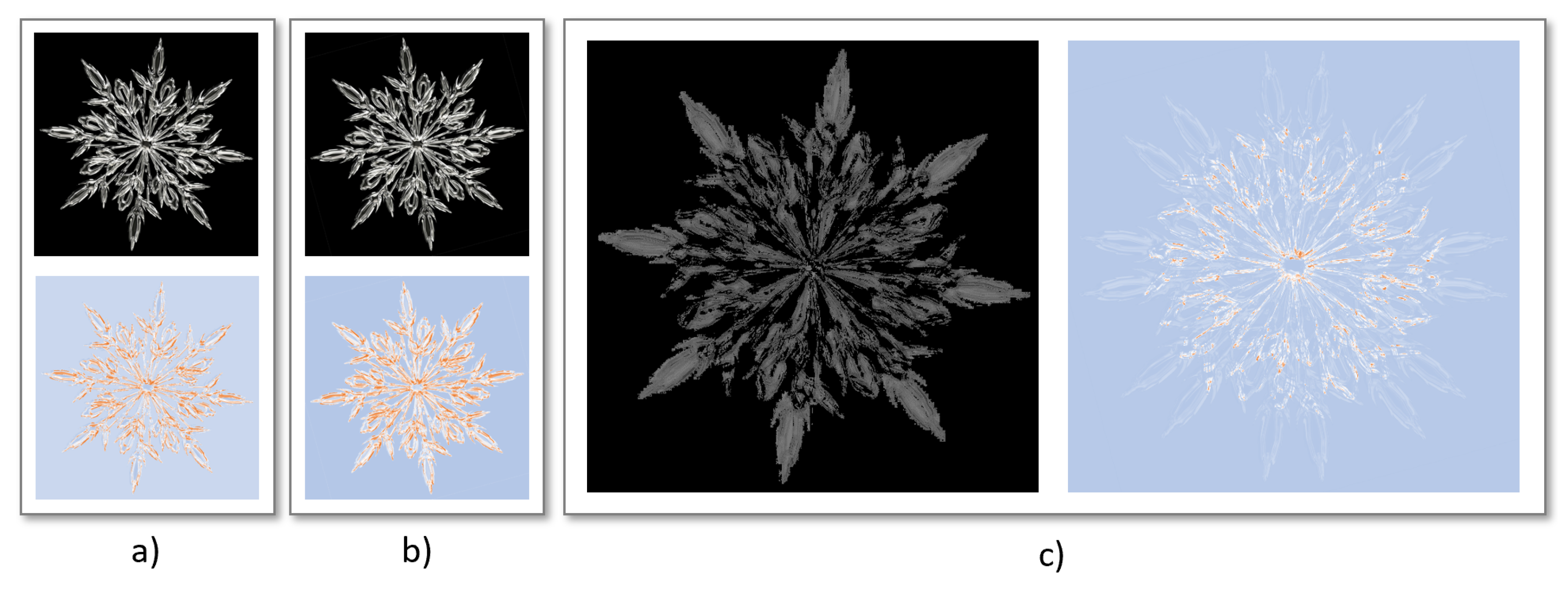
Figure 4 shows the result of an uncertainty-aware image comparison. Here,
Figure 4a,b show the input images that need to be compared and their uncertainty-quantification. Here, the goal is to identify image pixels in
Figure 4a that have an higher intensity value then the image in
Figure 4a.
Figure 4c shows the resulting comparison. Contrary to a binary comparison, where pixels can either be smaller or larger then the compared value, an uncertainty-aware comparison includes the probability of an image pixel to be higher, then the compared value. In addition to the output image, the resulting uncertainty can be reviewed as well.
4.3.2. Histogram Equalization
Histogram equalization is an important technique to increase the global contrast in an image [
39]. It works on the basis of a histogram counting the occurrences of intensity values in an image and equalizing them. To achieve this, the histogram
needs to be computed. For each possible intensity value it counts its occurrences in the entire image and equalizes these measures according to the number of pixels in the input image. More formally,
can be computed as:
where
z is the number of pixels in the image. Based on this histogram it is possible to define a mapping that projects each intensity value
x to a novel value
. This can be achieved by:
As it can be seen, the resulting histogram equalization is computed for each intensity value of the image. Therefore, this computation does not change the respective uncertainty information of the input image. Instead, the uncertainty information can refine the computation of the histogram. Therefore, an uncertainty-aware histogram
can be computed by:
This computation achieves that uncertain values are less strongly considered in the histogram. Although an image contains a huge amount of voxels with the same value, the respective ratio in the histogram can be relatively small when all counted values hold a high uncertainty.
Utilizing this equation, the histogram equalization in Equation (
12) can be changed, thus:
. The resulting histogram expansion is adjusted to the uncertainty-aware histogram.
Figure 5 shows the result of a histogram equalization when not considering uncertainty information and when considering uncertainty information. Starting from the input image in
Figure 5a, the histogram equalization for
Figure 5b shows a very light results where highlights are hard to identify. In contrast to this, the histogram equalization considering uncertainty information in
Figure 5c outputs improved results. Highlights can be seen easier and the overall appearance looks clearer.
4.3.3. Kernel Operations
A huge variety of pre-processing operations is based on kernels that allow a convolution of pixels [
40]. Kernels can be used to achieve a variety of tasks, such as smoothing or edge detection. When applying such a function, the kernel does not solely change the image itself. It also changes the uncertainty information of the underlying image.
In addition, the uncertainty information of a pixel can help adjusting the importance of different pixels considered for a convolution. Here, the goal is to increase the influence of certain values in a convolution while weakening the influence of uncertain pixels.
Let
k be a kernel and
n be the size of the kernel. Here, we assume quadratic kernels with a dimension of two. However, the principle can be easily extended to more general kernels.
Without considering uncertainty information, the kernel
k can be used to achieve a convolution of a voxel
and its surrounding
by :
As mentioned above, this definition does not consider the uncertainty of each each pixel. Therefore, the convolution of pixels through a kernel can be extended by:
This means that the weighted sum of the pixel values is not solely adjusted by the kernel itself. Instead, the sum is adjusted to increase the weight of pixels with low uncertainty and decrease the weight of pixels with high uncertainty.
In addition to the convolutional computation of the image, the uncertainty of the underlying image needs to be adapted as well by utilizing the equations presented in
Section 3. The influence of a convolution to the uncertainty of an image can then by computed by:
A prominent example for a kernel operation working on image data is the Gaussian smoothing operation. Therefore, a kernel size can be selected by a user that determines the radius around a voxel that are considered for the smoothing operation.
Another example of image operations that use kernels is the edge detection through a Laplace operator.
Figure 6b shows the result of an uncertainty-aware Gaussian smoothing according to an input image and its uncertainty
Figure 6a. Here, it become clear that the Gaussian smoothing is not solely modifying the image itself but additionally the underlying image uncertainty.
Figure 6c shows the result of an uncertainty-aware Laplace edge detection according to the input image and its uncertainty
Figure 6a. The result shows that the uncertainty-aware Laplace operator is able to express the uncertainty of a detected edge. In cases where the filter detects an edge on uncertain pixels, the responding edge will be seen clearly in the resulting image. In cases where the edge detection algorithm detects an edge according to underlying image pixels that are uncertain, the resulting edge is shown darker. Here, users can directly see which detected edges are certain and which are not. Additionally, the uncertainty of the input data is transformed as well.
4.4. Multiple Uncertainty-Aware Operators
As
Section 4.3 shows, image pre-processing operations can be adapted such that they consider the input uncertainty of an image. In addition, the uncertainty information of the input image is transformed as well.
In many cases, pre-processing is not a single operation. Instead, image pre-processing is an entire pipeline composed of multiple image pre-processing operations. In order to address this, this paper presents a system that allows users to select uncertainty-aware pre-processing operations and connect them in an arbitrary manner.
When creating new image pre-processing pipeline, the images are sorted chronologically which means that operations, which are computed first, are visualized first as well. Computational results that are based on one or multiple image inputs are connected through black arrows, respectively. The arrows contain a marker indicating the applied operation. Users are enabled to create new connections and define the image pre-processing technique that should be applied along this connection.
This allows an easy to understand visual mechanism for users in different domains to apply arbitrary uncertainty-aware image pre-processing techniques, build entire image pre-processing pipelines, and review the impact of each operation to the uncertainty of the input dataset.
5. Results
To show the effectiveness of the presented approach, this section presents successful applications of the uncertainty-aware pre-processing for real world datasets in medical imaging and satellite image analysis.
5.1. Sobel Operator
A basic example for such an operator is the detection of edges through the Sobel operator. Contrary to the Laplace operator, the Sobel operator is available in two versions. Each of them is detecting edges in one direction: x and y. After computing both of these operations, these need to be combined to a final image containing the edges of the underlying input image.
Figure 7 shows the propagation of uncertainty when applying the Sobel operator to an image. Figure reffig:sobelProp (top) Shows the input image and its uncertainty quantification when applying Gaussian error as an uncertainty measure.
Figure 7 (center) shows the results for the uncertainty-aware Sobel operator in
x and
y direction. For uncertain pixels that are classified as edges, the resulting edge is uncertain as well. In a final step, all edges in the image can be computed by combining the result from the sobel operator in
x and
y direction. The results do not solely show the uncertainty-aware computational steps of the presented pipeline. In addition, it shows how the uncertainty increases throughout the entire computation of the pipeline. Starting with a relatively low uncertainty throughout the input image, the resulting image contains pixels that are highly affected by uncertainty. In addition, the visualization indicates that the last step is the one causing the highest rise in uncertainty.
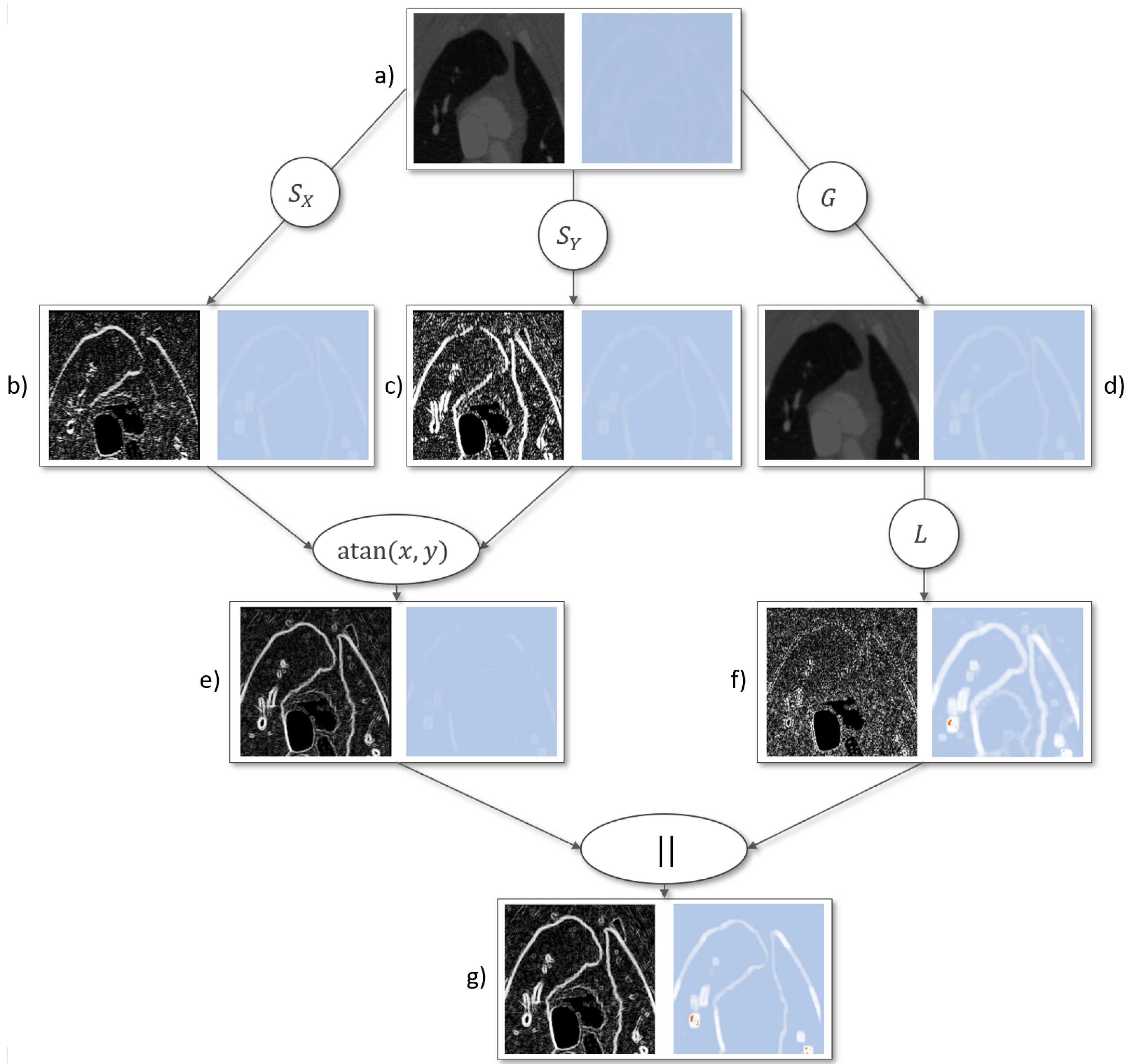
5.2. Medical Image Data
The second example is an edge detection scenario for medical image data. For further information on the data acquisition process, see [
41]. The CT scan has a size of 512 × 512 × 496 voxels capturing the upper thorax of a pig. The medical task for this dataset is to identify the vessels contained in the lung of the pig. On the input image, they can be identified as the white strings in the black areas (lung).
To achieve the uncertainty quantification, the following measures where utilized: contrast stretch and Gaussian error. The utilized pipeline can be reviewed in
Figure 8.
In this example, two edge detection algorithms where combined. First, the Sobel edge detection was utilized.
Figure 8b,c show the application of the Sobel kernel in
x and
y direction. After that, they are combined utilizing the length of vector function in
Figure 8. On the other hand, a Gaussian smoothing was applied to the original image
Figure 8d. After that, the Laplace edge detection was applied
Figure 8f. Finally, both edge detection results are combined utilizing the length of vector function
Figure 8g.
The intermediate computational results are sorted by their order of computation. It can be observed that the uncertainty in the image increases throughout the computation. Especially the pixels involved in edges are affected by uncertainty throughout the computation. In addition, it can be observed that the Laplace operator affects the uncertainty more in comparison to the Sobel operator computation. This can give a hint to users to choose a specific image operation that is better suited with respect to the resulting uncertainty.
Figure 8e shows less white and orange areas (medium and high uncertainty) in comparison to
Figure 8f. This is especially important as edges contain the highest amount of uncertainty in this example. With this knowledge, users are guided to select image operations that keep the amount of resulting uncertainty low.
When reviewing the final image and its uncertainty, it can be seen that the uncertainty-aware edge detection achieved an identification of the vessels in the pig’s lung. When considering the uncertainty of this computation, there are two vessel edges that appear highly uncertain. In the edge detection view, these edges are shown very thick. Here, it becomes clear that the exact location of the edge cannot be determined properly. This is the result of the partial volume effect that is likely to happen when capturing vessels due to the fact that the resolution is not high enough to clearly define the vessel boundary.
5.3. Satellite Images
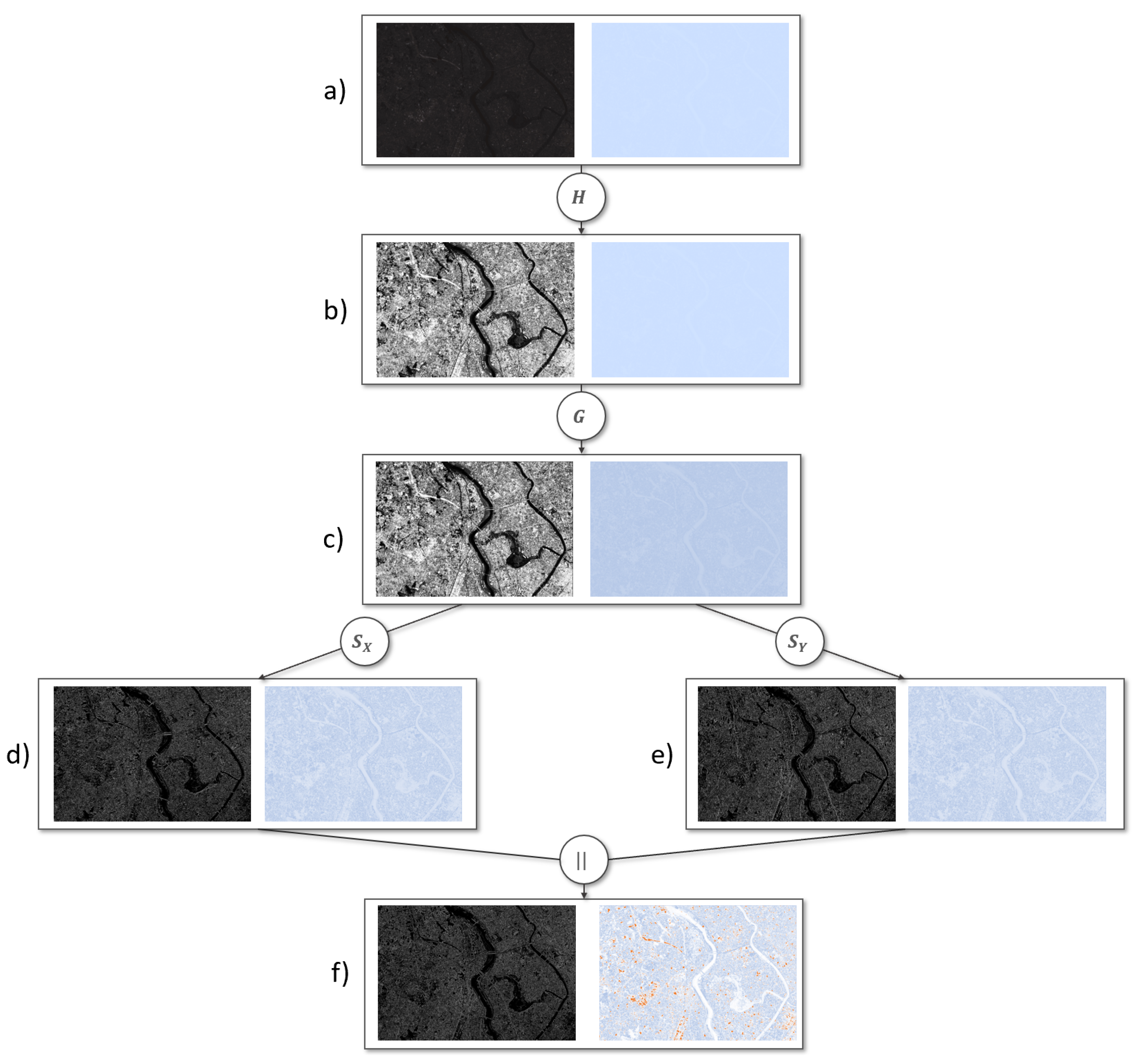
The final example is the examination of satellite images [
42]. In the presented example, the Tokyo area was captured. The results show a small part of the captured image. It has the size of 3000 × 2000 pixels and contains two rivers and a variety of houses. The overall goal for the presented image is to identify different types of buildings. Here, it is important to extract the edges of buildings in a series of pre-processing steps.
Figure 9 shows the resulting uncertainty-aware image pre-processing pipeline to achieve an edge detection of the input image in a). As is can be seen, the first image has insufficient contrast. Resulting from that, the first step in the pre-processing pipeline was to apply a contrast equalization. After that, a Gaussian smoothing with a 5 × 5 kernel was applied to remove noise from the image. Furthermore, both Sobel operators (x and y direction) where applied. In a final step, the outputs of the Sobel operator where combined by computing the length of the vector containing the result of the Sobel operators. For each step, the visualization includes the result of the computational step as an image as well as the uncertainty depending on the previous image pre-processing operations. As an uncertainty-measure, the local contrast measure was utilized.
The example shows that the uncertainty increases throughout the computation of the pre-processing pipeline. While the uncertainty quantification in the input image is really low, it increases throughout the computation. It can be observed that this increase is not equally distributed in the image. Specific structures, such as the rivers and distinct buildings, are affected more by uncertainty.
Figure 10 shows a closeup for the final result of the pre-processing pipeline and its uncertainty. Here, it can be observed that the uncertainty-aware Sobel operator was able to output all sorts of edges in the input images. Depending on the underlying uncertainty, the resulting edges are certain (white) and uncertain (light gray). Applying a threshold can help users to find edges that are certain enough for further analysis.
The respective uncertainty visualization shows that the captured edges of the rivers are highly certain whereas there appear a variety of buildings containing uncertain edges. For further analysis of these edges, this is an important information that can refine the following computation. Users can decide to apply a threshold that selects the most certain edges and continue their computation based on the thresholded edges. Still, all detected edges can be utilized for further analysis of the image. In case the following operation is uncertainty-aware, the presented result of the edge detection can be utilized. Here, edges that are detected as uncertain would lead to houses that are detected with a certain level of uncertainty. This allows users to rate their overall computational results in terms of uncertainty.
The example shows that users can easily build their own pipelines and review how the overall uncertainty in an image changes. The visual representation of the user-defined pipeline is intuitive and the chronology of the operations is easy to follow. The result also shows that the Laplace operator is changing the uncertainty of the image more than the Sobel operator does. Here, users can decide if this is a desired behavior or if they want to rely on the Sobel edge detection as it is less uncertain.
6. Discussion
In the following section, we will discuss the summarized requirements for an uncertainty-aware visual system for image pre-processing including the uncertainty principles and the requirements to promote a successful visualization in application areas. We showed that related approaches are solely able to address an uncertainty-awareness or a visualization of uncertainty. The presented approach is designed to build a bridge between these two areas as shown below.
6.1. Discussion of Uncertainty Principle
In this section, we discuss the ability of the presented approach to achieve complete uncertainty awareness.
C1: Quantify uncertainty in each component. The presented methodology is able to quantify the uncertainty of each image pixel. Here, we utilize different error measures to create an arbitrary high-dimensional uncertainty space capturing multiple aspects of uncertainty. Users are enabled to select the utilized error measures to achieve an uncertainty quantification that meets their needs and fits to the underlying image data best.
C2: Visualize uncertainty information. In the presented methodology, visualization is a key concept. Each computational step and its uncertainty is visually presented. Here, users can select from three different visualization modes depending on the visualization purpose.
C3: Enable interactive uncertainty exploration. As shown in the presented results, our methodology allows an interactive composition of multiple uncertainty-aware image pre-processing operations. All parameters and settings can be selected by the user. Users can choose steps and regions they are particularly interested in.
C4: Propagate and aggregate uncertainty. The propagation and aggregation of uncertainty is ensured by refining a variety of image preprocessing algorithms such that they are able to transform the image properly. This means that the image pre-processing operations are including uncertainty information throughout their computation. In addition, the presented operations are able to adjust the underlying image’s uncertainty as well. The presented system is designed such that these transformations are propagated along arbitrary image pre-processing pipelines.
6.2. Discussion of Requirements for a Real World Use
Usability, effectiveness, correctness, intuitiveness, and flexibility are known to be key factors that promote a real world use of a visualization system [
25]. In the following section, we will discuss the ability of the presented approach to meet these requirements.
M1: Usability. The presented methodology is easy to use for domain scientists as is allows to generate arbitrary pre-processing pipelines. The visualization and arrangement of individual computational steps help users to understand the composition of the single steps and how they change the underlying uncertainty. Visualization types can be chosen according to individual needs.
M2: Effectiveness. The effectiveness of the presented methodology is ensured although the additional information needs to be stored and computed. When considering n as the number of pixels, the required storage for the presented methodology is , where q is the number of uncertainty measures and r the number of computations selected by the users. The computational effort is highly depending on the underlying image operation. When assuming O as an upper bound of all utilized image operations, the resulting runtime complexity can be expressed by . For both, storage efficiency and runtime efficiency, the presented methodology solely adds a linear factor. In many related approaches, the runtime exceeds linearity. In addition, the approach can be parallelized as different cores do not require the input image in its entirety.
M3: Correctness. As the results show, the presented uncertainty-aware image pre-processing operations output correct results, such as the classic versions of each operator does. In addition it provides a refinement of these operators that allows to express the uncertainty of the computational result.
M4: Intuitiveness. The presented methodology is intuitive as it allows an easy to understand selection and connection process of the provided uncertainty-aware pre-processing operations. The computational results are sorted by their order to allow an intuitive reviewing by users.
M5: Flexibility. The flexibility of our system is high as we allow a variety of uncertainty measures and their combination. The presented system additionally allows the inclusion of further uncertainty measures. Furthermore, it is able to handle datasets that already have an uncertainty quantification. For the visualization of the uncertainty quantification in each step, we allow three different visualization types: juxtaposition, superposition, and embedded iso-surface visualizations. Furthermore, the methodology is not restricted in terms of image data that can be utilized as input. 2D or 3D images, color-images or grey-scale, and different image types can be considered. Still, an extension of the visualization methodologies would be required when considering 3D images [
43]. In such cases, visual clutter can occur and a proper visualization strategy for uncertain pixels need to be found. A further limitation of the presented approach can be reached, when images became very large. At some point, not all intermediate steps can be displayed at the same time without a huge zoom factor. Here, focus and context approaches, such as hierarchical clustering, are required [
44]. The flexibility of the presented methodology can be increased further when adding new uncertainty-aware image pre-processing operations. The code is designed such that users are able to implement new operations when required regarding the given uncertainty-propagation principles.
7. Conclusions
This work presents an uncertainty-aware pre-processing methodology that combines two important features: the correct propagation of uncertainty throughout image pre-processing operations and a visual system to review image pre-processing steps and their uncertainty. To achieve this, the rules for uncertainty propagation were carefully summarized and applied to common pre-processing techniques. These operations are able to transform the underlying image properly, express the certainty of the computation and transform the images’ uncertainty as well. In order to allow users to build arbitrary image pre-processing pipelines, the presented approach offers a flexible visual system. In this system, users can follow the changes of the image throughout the selected image pre-processing pipeline. The methodology was successfully applied to a variety of real world datasets showing its effectiveness.
Author Contributions
Conceptualization, C.G. and P.A.; Methodology, C.G.; Validation, Thomas Wischgoll; Formal Analysis, C.G.; Resources, J.T.H.; Data Curation, T.W.; Writing—Original Draft Preparation, C.G.; Writing—Review & Editing, T.W. and P.A.; Visualization, C.G.; Supervision, J.T.H.; Project Administration, H.H.; Funding Acquisition, H.H.
Funding
This research received no external funding.
Acknowledgments
The authors would like to thank PlanetLabs for providing the satellite imagery of the Tokyo area through our free research license.
Conflicts of Interest
The authors declare no conflict of interest.
References
- Sonka, M.; Hlavac, V.; Boyle, R. Image pre-processing. In Image Processing, Analysis and Machine Vision; Springer: Boston, MA, USA, 1993; pp. 56–111. [Google Scholar]
- Ekman, U.; Agostinho, D.; Thylstrup, N.B.; Veel, K. The uncertainty of the uncertain image. Digit. Creat. 2017, 28, 255–264. [Google Scholar] [CrossRef]
- Gillmann, C.; Wischgoll, T.; Hagen, H. Uncertainty-Awareness in Open Source Visualization Solutions. In Proceedings of the IEEE Visualization Conference (VIS)—VIP Workshop, Baltimore, MD, USA, 23–28 October 2016. [Google Scholar]
- Wilson, R.; Granlund, G.H. The Uncertainty Principle in Image Processing. IEEE Trans. Pattern Anal. Mach. Intell. 1984, PAMI-6, 758–767. [Google Scholar] [CrossRef]
- PAL, S.K. Fuzzy image processing and recognition: uncertainty handling and applications. Int. J. Image Gr. 2001, 1, 169–195. [Google Scholar] [CrossRef]
- Mencattini, A.; Rabottino, G.; Salicone, S.; Salmeri, M. Uncertainty handling and propagation in X-ray images analysis systems by means of Random-Fuzzy Variables. In Proceedings of the 2008 IEEE International Workshop on Advanced Methods for Uncertainty Estimation in Measurement, Trento, Italy, 21–22 July 2008; pp. 50–55. [Google Scholar] [CrossRef]
- Ji, Q.; Haralick, R.M. Error propagation for the Hough transform. Pattern Recognit. Lett. 2001, 22, 813–823. [Google Scholar] [CrossRef]
- Davis, T.J.; Keller, C.P. Modelling and Visualizing Multiple Spatial Uncertainties. Comput. Geosci. 1997, 23, 397–408. [Google Scholar] [CrossRef]
- Yi, S.; Haralick, R.M.; Shapiro, L.G. Error propagation in machine vision. Mach. Vis. Appl. 1994, 7, 93–114. [Google Scholar] [CrossRef]
- Krishnapuram, R.; Keller, J.M. Fuzzy set theoretic approach to computer vision: An overview. In Proceedings of the IEEE International Conference on Fuzzy Systems, San Diego, CA, USA, 8–12 March 1992; pp. 135–142. [Google Scholar] [CrossRef]
- Rangarajan, C.; Jayaramamurthy, S.; Huntsberger, T. Representation of Uncertainty in Computer Vision Using Fuzzy Sets. IEEE Trans. Comput. 1986, 35, 145–156. [Google Scholar] [CrossRef]
- Haralick, R.M. Propagating Covariance in Computer Vision. In Performance Characterization in Computer Vision; Klette, R., Stiehl, H.S., Viergever, M.A., Vincken, K.L., Eds.; Springer: Dordrecht, The Netherlands, 2000; pp. 95–114. [Google Scholar]
- Hua, M.; Pei, J. Probabilistic Path Queries in Road Networks: Traffic Uncertainty Aware Path Selection. In Proceedings of the 13th International Conference on Extending Database Technology, Lausanne, Switzerland, 22–26 March 2010; pp. 347–358. [Google Scholar] [CrossRef]
- Stachowiak, A.; Żywica, P.; Dyczkowski, K.; Wójtowicz, A. An Interval-Valued Fuzzy Classifier Based on an Uncertainty-Aware Similarity Measure. In Intelligent Systems’2014; Angelov, P., Atanassov, K., Doukovska, L., Hadjiski, M., Jotsov, V., Kacprzyk, J., Kasabov, N., Sotirov, S., Szmidt, E., Zadrożny, S., Eds.; Springer International Publishing: Cham, Switzerland, 2015; pp. 741–751. [Google Scholar]
- Bonneau, G.P.; Hege, H.C.; Johnson, C.R.; Oliveira, M.M.; Potter, K.; Rheingans, P.; Schultz, T. Overview and State-of-the-Art of Uncertainty Visualization. In Scientific Visualization: Uncertainty, Multifield, Biomedical, and Scalable Visualization; Hansen, C.D., Chen, M., Johnson, C.R., Kaufman, A.E., Hagen, H., Eds.; Springer: London, UK, 2014; pp. 3–27. [Google Scholar]
- Lundström, C.; Ljung, P.; Persson, A.; Ynnerman, A. Uncertainty Visualization in Medical Volume Rendering Using Probabilistic Animation. IEEE Trans. Vis. Comput. Gr. 2007, 13, 1648–1655. [Google Scholar] [CrossRef] [PubMed]
- Fleßner, M.; Müller, A.; Götz, D.; Helmecke, E.; Hausotte, T. Assessment of the single point uncertainty of dimensional CT measurements. In Proceedings of the 6th Conference on Industrial Computed Tomography, Wels, Austria, 9–12 February 2016. [Google Scholar]
- Wong, P.C.; Bergeron, R.D. 30 Years of Multidimensional Multivariate Visualization. In Scientific Visualization, Overviews, Methodologies, and Techniques; IEEE Computer Society: Washington, DC, USA, 1997; pp. 3–33. [Google Scholar]
- Ding, Z.; Ding, Z.; Chen, W.; Chen, H.; Tao, Y.; Li, X.; Chen, W. Visual inspection of multivariate volume data based on multi-class noise sampling. Vis. Comput. 2016, 32, 465–478. [Google Scholar] [CrossRef]
- Akiba, H.; Ma, K.L.; Chen, J.H.; Hawkes, E.R. Visualizing Multivariate Volume Data from Turbulent Combustion Simulations. Comput. Sci. Eng. 2007, 9, 76–83. [Google Scholar] [CrossRef]
- Ma, K.; Lum, E.B.; Muraki, S. Recent advances in hardware-accelerated volume rendering. Comput. Gr. 2003, 27, 725–734. [Google Scholar] [CrossRef]
- Gillmann, C.; Arbeláez, P.; Hernández, J.T.; Hagen, H.; Wischgoll, T. Intuitive Error Space Exploration of Medical Image Data in Clinical Daily Routine. In EuroVis 2017—Short Papers; Kozlikova, B., Schreck, T., Wischgoll, T., Eds.; The Eurographics Association: Lyon, France, 2017. [Google Scholar] [CrossRef]
- Sacha, D.; Senaratne, H.; Kwon, B.C.; Ellis, G.; Keim, D.A. The Role of Uncertainty, Awareness, and Trust in Visual Analytics. IEEE Trans. Vis. Comput. Gr. 2016, 22, 240–249. [Google Scholar] [CrossRef] [PubMed]
- Maack, R.G.C.; Hagen, H.; Gillmann, C. Evaluation of the uncertainty-awareness principleusing a tumor detection scenario. In Proceedings of the VisGuides: 2nd Workshop on the Creation, Curation, Critique and Conditioning of Principles and Guidelines in Visualization (IEEE Vis 2018), Berlin, Germany, 21–22 October 2018. [Google Scholar]
- Gillmann, C.; Leitte, H.; Wischgoll, T.; Hagen, H. From Theory to Usage: Requirements for successful Visualizations in Applications. In Proceedings of the IEEE Visualization Conference (VIS)—C4PGV Workshop, Baltimore, MA, USA, 23 October 2016. [Google Scholar]
- Taylor, J. Introduction To Error Analysis: The Study of Uncertainties in Physical Measurements; A Series of Books in Physics; University Science Books: South Orange, NJ, USA, 1997. [Google Scholar]
- Rumelhart, D.; Hinton, G.; Williams, R.; University of California, S.D.I.f.C.S. Learning Internal Representations by Error Propagation; ICS Report; Institute for Cognitive Science; University of California: San Diego, CA, USA, 1985. [Google Scholar]
- Gertsbakh, I. Measurement Uncertainty: Error Propagation Formula. In Measurement Theory for Engineers; Springer: Berlin/Heidelberg, Germany, 2003; pp. 87–94. [Google Scholar]
- Bevington, P.R.; Robinson, D.K. Data Reduction and Error Analysis for the Physical Sciences, 3rd ed.; McGraw-Hill: New York, NY, USA, 2003. [Google Scholar]
- Nguyen, H.T. A Survey of Uncertainty Measures: Structures and Applications. In Proceeding of the 1984 American Control Conference, San Diego, CA, USA, 6–8 June 1984; pp. 549–553. [Google Scholar] [CrossRef]
- Artmann, U. Image quality assessment using the dead leaves target: experience with the latest approach and further investigations. Proc. SPIE 2015, 9404, 94040J. [Google Scholar]
- Pizer, S.M.; Amburn, E.P.; Austin, J.D.; Cromartie, R.; Geselowitz, A.; Greer, T.; Romeny, B.T.H.; Zimmerman, J.B. Adaptive Histogram Equalization and Its Variations. Comput. Vis. Gr. Image Process. 1987, 39, 355–368. [Google Scholar] [CrossRef]
- Fienup, J.R. Invariant error metrics for image reconstruction. Appl. Opt. 1997, 36, 8352–8357. [Google Scholar] [CrossRef] [PubMed]
- Boyat, A.K.; Joshi, B.K. A Review Paper: Noise Models in Digital Image Processing. arXiv, 2015; arXiv:1505.03489. [Google Scholar] [CrossRef]
- L, J.V.; Gopikakumari, R. Article: IEM: A New Image Enhancement Metric for Contrast and Sharpness Measurements. Int. J. Comput. Appl. 2013, 79, 1–9. [Google Scholar]
- Tian, Q.; Xue, Q.; Sebe, N.; Huang, T. Error metric analysis and its applications. Proc. SPIE Int. Soc. Opt. Eng. 2004, 5601, 46–57. [Google Scholar]
- Irum, I.; Sharif, M.; Raza, M.; Mohsin, S. A Nonlinear Hybrid Filter for Salt & Pepper Noise Removal from Color Images. J. Appl. Res. Technol. 2015, 13, 79–85. [Google Scholar]
- Sahoo, P.; Soltani, S.; Wong, A. A survey of thresholding techniques. Comput. Vis. Gr. Image Proc. 1988, 41, 233–260. [Google Scholar] [CrossRef]
- Zuiderveld, K. Graphics Gems IV; Chapter Contrast Limited Adaptive Histogram Equalization; Academic Press Professional, Inc.: San Diego, CA, USA, 1994; pp. 474–485. [Google Scholar]
- Shawe-Taylor, J.; Cristianini, N. Kernel Methods for Pattern Analysis; Cambridge University Press: New York, NY, USA, 2004. [Google Scholar]
- Huo, Y.; Choy, J.S.; Wischgoll, T.; Luo, T.; Teague, S.D.; Bhatt, D.L.; Gebab, G.S. Computed tomography-based diagnosis of diffuse compensatory enlargment of coronary arteries using scaling power laws Interface. J. R. Soc. Interface 2002, 10, H514–H523. [Google Scholar]
- Planet Team. Planet Application Program Interface: In Space for Life on Earth; Planet Team: San Francisco, CA, USA, 2017; Available online: https://api.planet.com (accessed on 28 August 2018 ).
- Djurcilov, S.; Kim, K.; Lermusiaux, P.; Pang, A. Visualizing Scalar Volumetric Data with Uncertainty. Comput. Gr. 2002, 26, 239–248. [Google Scholar] [CrossRef]
- Chen, Z.; Healey, C. Large Image Collection Visualization Using Perception-Based Similarity with Color Features. In International Symposium on Visual Computing; Springer: Cham, Switzerland, 2016; pp. 379–390. [Google Scholar]
© 2018 by the authors. Licensee MDPI, Basel, Switzerland. This article is an open access article distributed under the terms and conditions of the Creative Commons Attribution (CC BY) license (http://creativecommons.org/licenses/by/4.0/).


