Use of an Occlusion Mask for Veiling Glare Removal in HDR Images

Abstract

Optical systems in digital cameras present a limit during the acquisition of standard and High Dynamic Range Images (HDRI) due to the presence of veiling glare, an artifact caused by an unwanted spread of the source of light. In this paper, we analyze the state-of-the-art of veiling glare removal in HDRI, giving attention to the paper presented by Talvala. Then we describe an algorithm for veiling glare removal based on the same occlusion mask, to study the benefits provided by it in HDRI acquisition process. Finally, we demonstrate the efficiency of the occlusion mask method in veiling glare removal without any post production estimation and subtraction.

1. Introduction

An HDRI (High Dynamic Range Image) is a digital image that represents a greater range of luminance levels than those obtained using a traditional sensor with a single exposure. HDRI acquisition techniques are based on a combination of several pictures of the same scene shot with different exposition parameters: doing that it’s possible to include in a single image a larger amount of luminance values that in a Low Dynamic Range Image (LDRI) would be lost due to the quantization limit. This imaging technique is particularly used in science, photography [1] and medicine.

The capability of a camera to shoot an HDRI is limited by veiling glare [2]. Veiling glare is a global illumination effect caused by multiple light dispersions inside the camera’s optical system. Veiling glare is different from the lens flare phenomenal: the second one appears when a punctiform and intense light source introduces in the image geometrical artifacts well defined; the veiling glare is instead related to extended sources of light and is similar to a blurred lens flare: it can be also caused by light sources out of the field of view but in this case it can be avoided using a lens hood.

Ideally, a punctiform light source should illuminate a single pixel of the sensor, but in reality it also affects the pixels in the proximity, with an intensity proportional to the distance from the correct pixel and to the quality of the lens. The 2D function that describes the intensity of this phenomena is the Glare Spread Function (GSF) of the lens (Figure 1).

Figure 1. Example of Glare Spread Function (GSF).

In Section 2 will be presented the state-of-the-art and some techniques of veiling glare removal during the acquisition and post-processing phases. In Section 3 will be described a technique of veiling glare removal based on spatial grid; in Section 4 will be presented the algorithm that we used to reconstruct the images, its implementation, testing and results. At last, in Section 5 will be discussed the limits and possible future developments of the technique proposed.

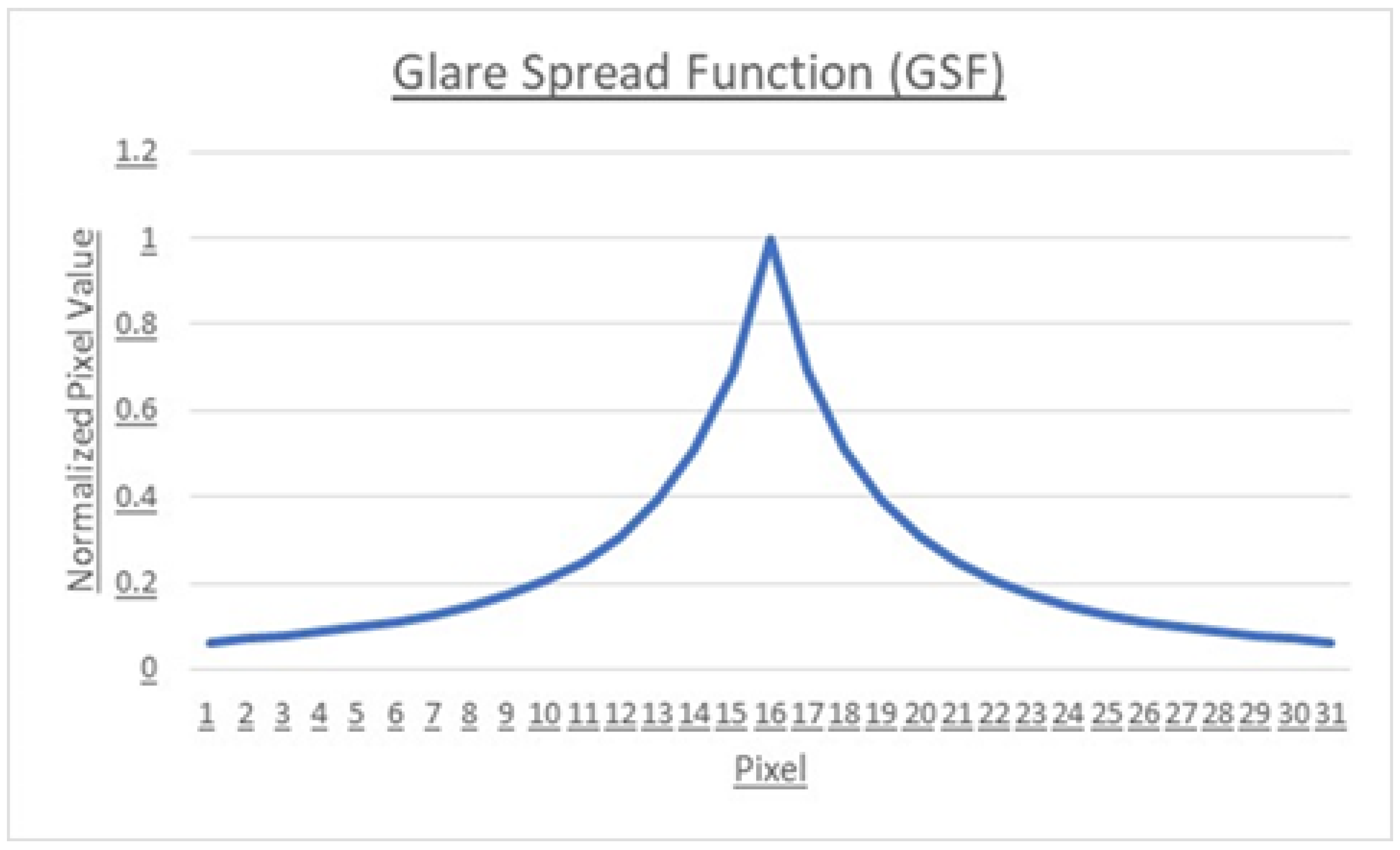
2. State-of-the-art

Most of veiling glare removal techniques are focalized on refining optical elements of the system, for example improving the lenses coating [3]. Other methods are instead based on post-processing techniques, removing the veiling glare from images that are already affected by it. A common approach is using deconvolution techniques on the image, as presented in Starck et al. [4].

One deconvolution method for the veiling glare removal in post-processing is illustrated by Talvala et al. [5]: this technique is based on the hypothesis that the GSF is space-invariant and consecutively that exist only one GSF for the image; this GSF convoluted with the scene creates the image with the veiling glare. However, while trying to correct the image with the deconvolution we will incur in two main problems: first, the image parts characterized by the presence of glare become too much noisy due to the quantization limit; second, glare residual remains, characterized by a different chromatic component in various zones. Talvala et al. [5] conclusion is that in the image there isn’t enough information for a successful veiling glare removal in post-production.

Nayar et al. [6] find as a correct approach for the veiling glare removal the separation between direct and global light, using a structured illumination and/or an occlusion mask (Figure 2). From this, Talvala et al. [5] develop their idea proposing the usage of an high frequency grid as occlusion mask. In the next section this method will be discussed and a variant of it will be proposed, in order to demonstrate the direct influence of the grid on the veiling glare.

Figure 2. Subdivision of light in three different component [6]: direct light (blue) global light from the scene (red) and global light from the camera lens (green).

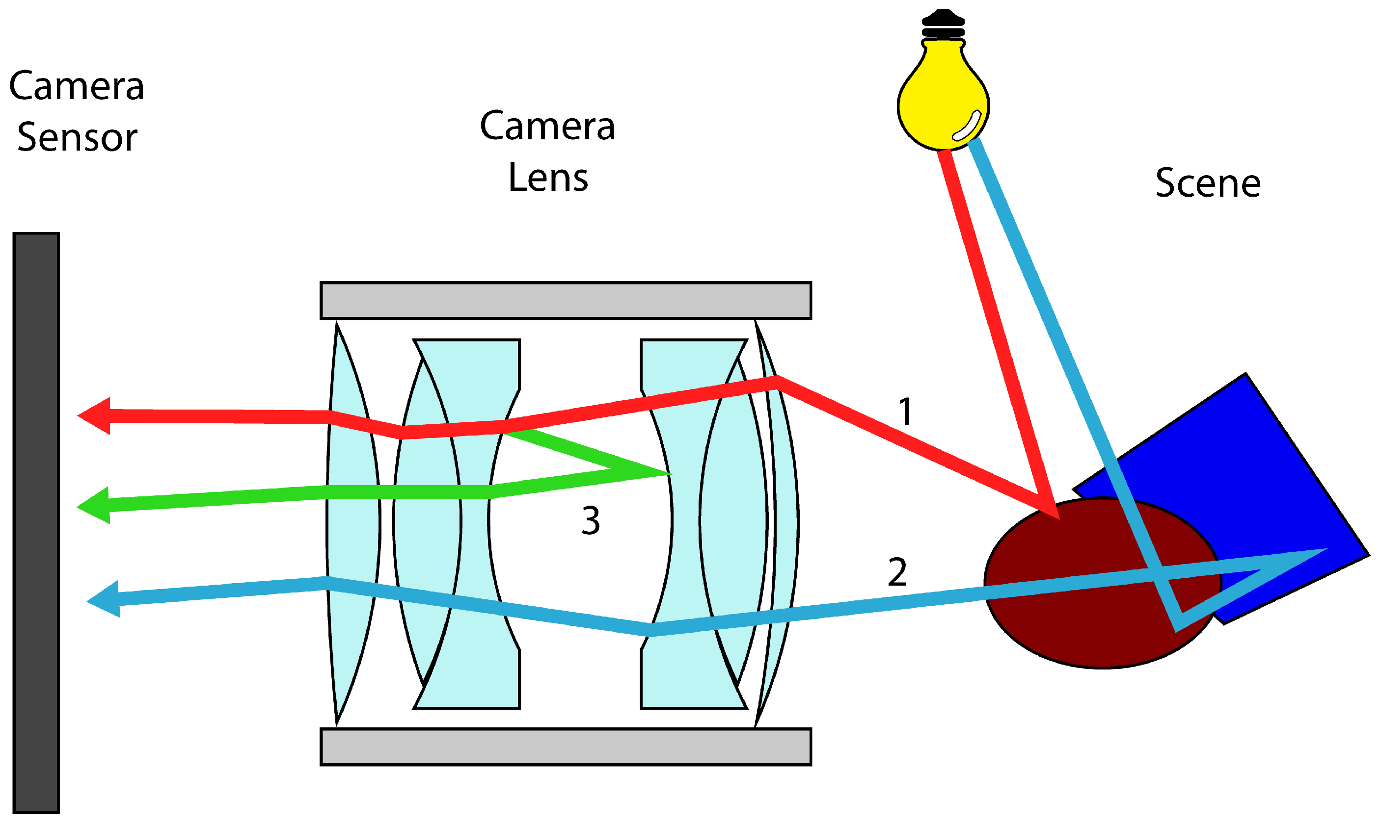
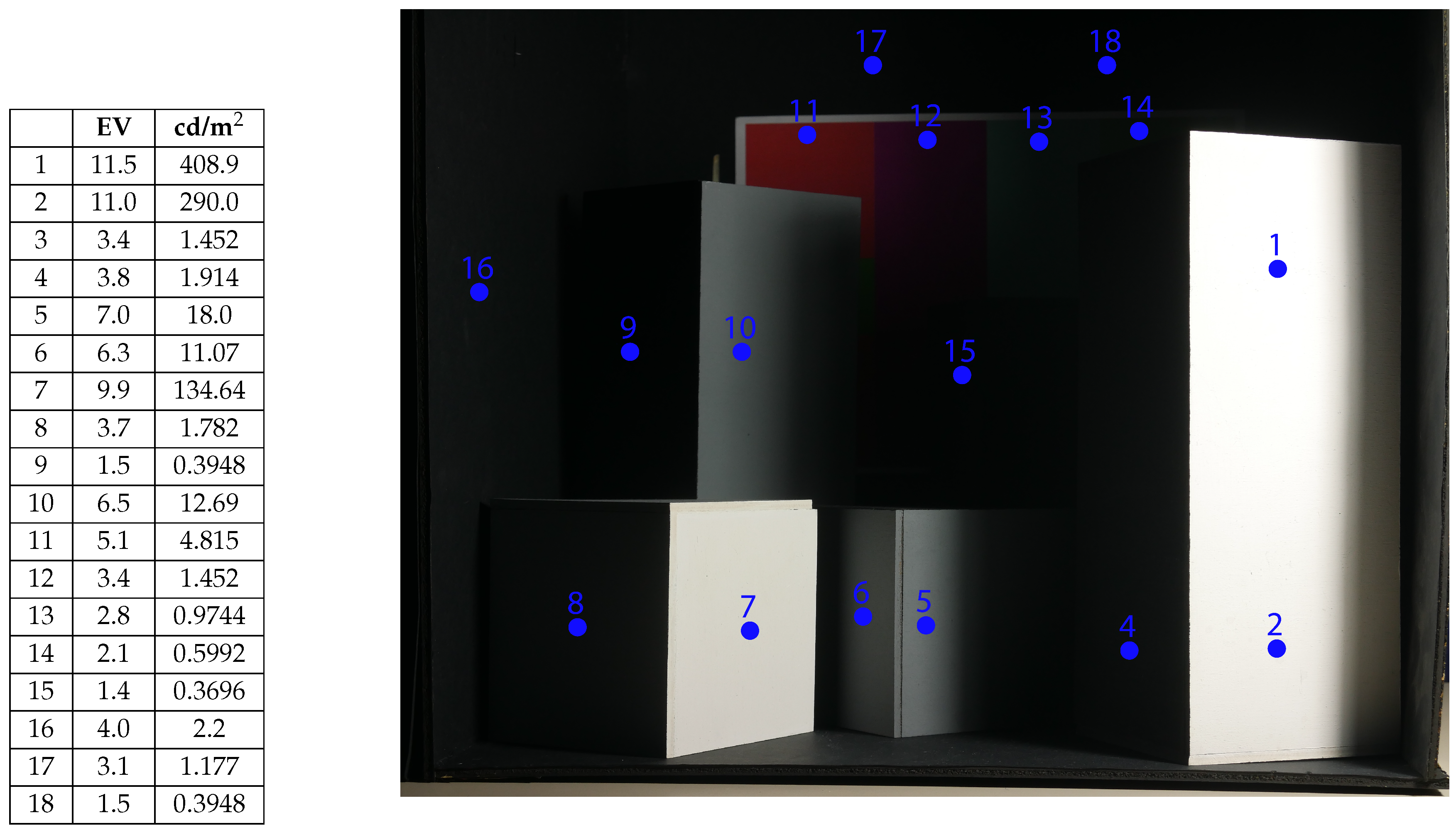
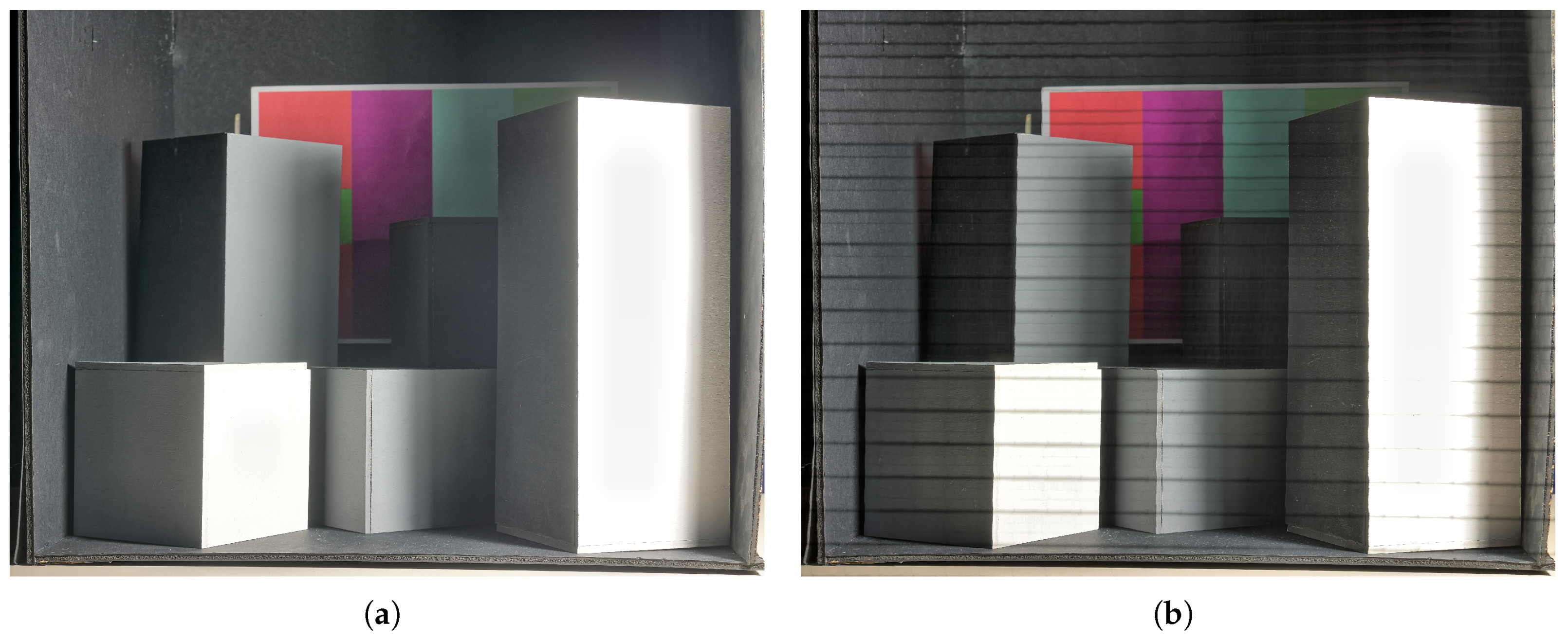
3. Occlusion Mask

Talvala et al. [5] placed a high-frequency occlusion mask between the camera and the scene to limit the presence of global light in the image (Figure 3). Since glare is composed only by low spatial frequencies, they used a grid with an average occlusion factor of $\alpha$ to reduce the amount of veiling glare recorded in every pixel by a factor of $\alpha$. It is necessary to shoot multiple captures, translating the mask in both directions (vertical and horizontal). This process is necessary to record only the direct component of light in all the scene. For a given $\alpha$, at east $1/\alpha$ captures are needed to represent the entire scene through unoccluded regions. A small $\alpha$ involve in an elevated number of captures but also a smaller amount of glare and global illumination component. A large $\alpha$ grants a quick capture at the cost of increasing the noise. These are the reasons why a tradeoff is necessary. In their work, they create an HDR image for each grid position. Then, they estimate the amount of veiling glare in the occluded regions center. Next, a Gaussian filter is applied to spread the glare in the entire image. Finally, they subtract the estimated glare from the original image, and discard the regions outside the mask holes to realize a new glare-free image. The purpose of our project is to evaluate the effectiveness of the occlusion mask in an High Dynamic Range Image observing how veiling glare is reduced without an estimation and a subtraction, considering not occluded regions only.

Figure 3. Structure and grid used in experiment.

4. Implementation

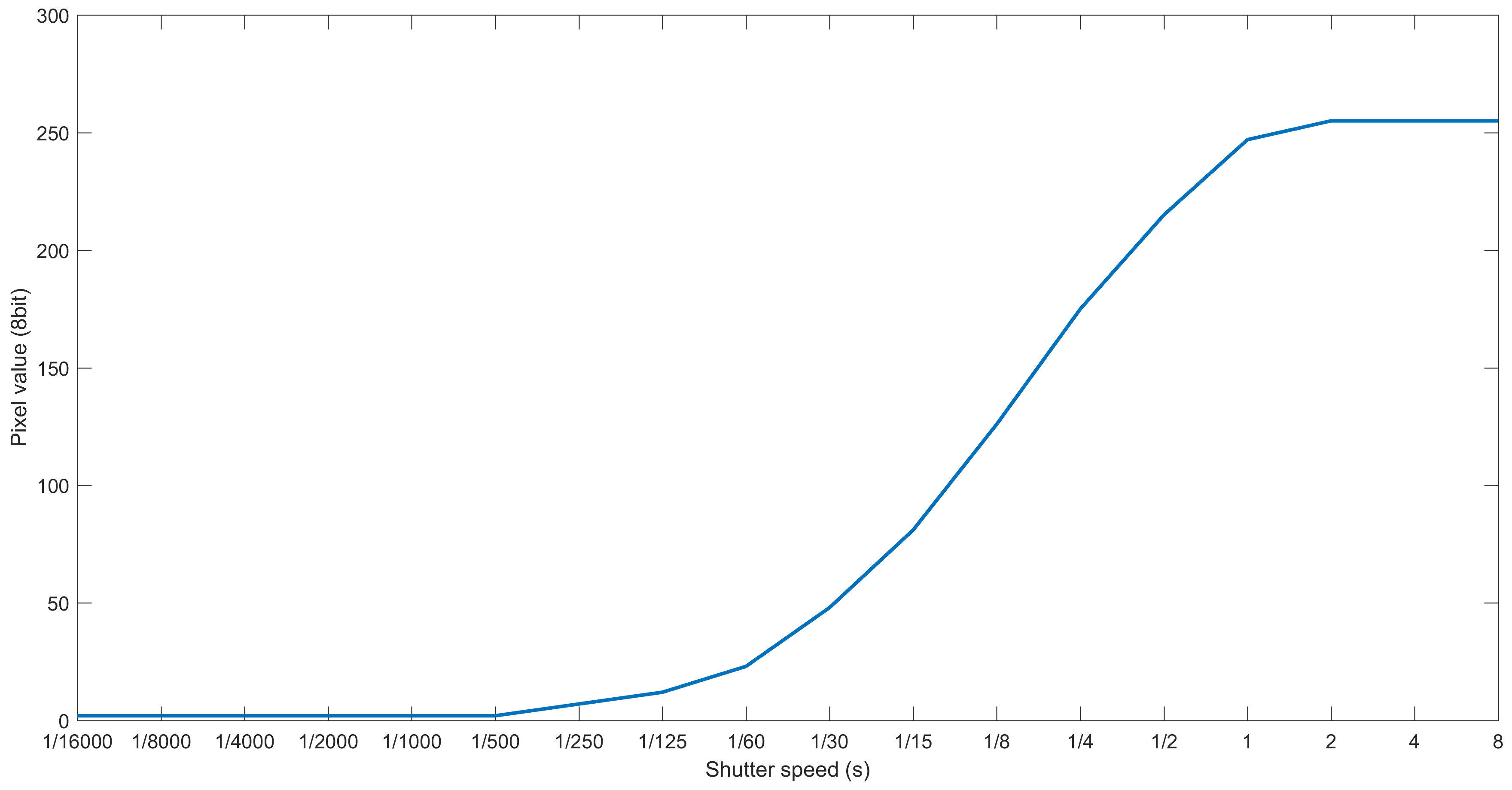
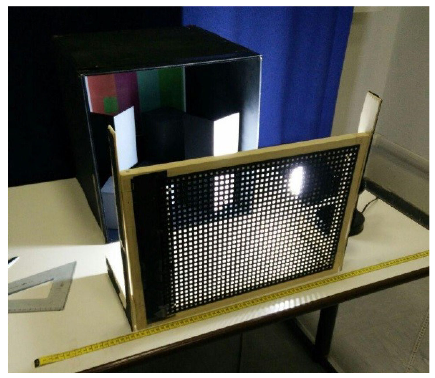
4.1. Acquisition

4.1.1. Grid and Materials

Based on the work of Talvala et al. [5] we used, as occlusion mask, an A3 matte black cardboard, laser cut as a grid with holes of 4 × 4 mm and a 1 cm period which leads to have an occlusion factor of $\alpha$ = 0.16. This factor allow us to reconstruct the whole image. The grid has been positioned as near as possible to the scene (to make sure that, while focusing the scene, the grid wouldn’t be too much blurred) with the help of a wooden structure as support. The grid has been horizontally moved 13 times, 1 mm at a time, while for the vertical movements we used 4 thicknesses to raise the grid. Figure 3 shows the grid and the structures used in the experiment.

4.1.2. Camera and Shot Settings

The final HDR image is composed by 7 images (with a range of exposition from −3 ev to +3 ev), each of them reconstructed starting from 13 × 4 images (13 horizontal steps × 4 vertical steps) of the scene occluded by the grid. In total we shot 364 photos. The pictures have been shot with a mirrorless Panasonic Lumix G7 (Panasonic, Osaka Prefecture, Japan) with a m4/3 sensor of 16 Megapixels, and a 14–42 mm lens (equivalent to a 28–84 mm in a 35 mm sensor) f/3.5–5.6. The characteristic curve of the optical system used is showed in Figure 4. The images are acquired with parameters shown in Table 1.

Figure 4. Characteristic curve of camera used (Lumix G7). To construct it we have photographed a white wall keeping an aperture of f8 and varying exposure times from about 1/1,6000 to 8 s. We have then obtained the intensity for each photo, plotted obtained values on the Y-axis, and time on X.

Table 1. Shooting Settings.

	EV -3	EV -2	EV -1	EV 0	EV 1	EV 2	EV 3
FOCAL LENGTH	35 mm (eq. 70 mm)	35 mm (eq. 70 mm)	35 mm (eq. 70 mm)	35 mm (eq. 70 mm)	35 mm (eq. 70 mm)	35 mm (eq. 70 mm)	35 mm (eq. 70 mm)
ISO	400	400	400	400	400	400	400
F-STOP	8.0	8.0	8.0	8.0	8.0	8.0	8.0
SHUTTER SPEED	1/8	1/4	1/2	1	2	4	8

The scene is composed by several cubes and parallelepipeds of various grey tones, inserted in a wooden box with black walls that can block the ambient light. The scene is illuminated with a lamp with a color temperature of 6400K expressly screened to not illuminate the grid, as it would cause more glare and a big amount of noise during the reconstruction phase (see after). On the background of the scene has been set an A4 sheet with different colored sections. Figure 5 shows the scene photographed with the different luminance values measured in several points.

Figure 5. Luminance value record.

4.2. Reconstruction Technique

At the end of the acquisition phase, the next step is to reconstruct the image of the scene assembling the areas not occluded by the mask. For each of the 7 exposures, we have taken a total of 52 photos (13 × 4): this means that we have collected, for each pixel $P_{\mathrm{I}}$ of the final image 52 values. Reconstructing the image without an occlusive mask means assigning to each pixel $P_{\mathrm{I}}$ the value assumed when not occluded.

Let’s call $F_{\mathrm{P}}$ the set of 52 values $f\left(P_{\mathrm{I}}\right)$ assumed by every pixel $P_{\mathrm{I}}$: we started considering the histogram of $F_{\mathrm{P}}$ to understand which values $f\left(P_{\mathrm{I}}\right)$ represent the occluding mask and which ones represent the scene and must be used in the final reconstructed image. Ideally, every pixel should assume only two different values, one for the occluding mask and one for the scene: obviously, in a real context with the presence of non-sharp edges of the un-occluded zones, we expected to notice a bimodal distribution of the values of $F_{\mathrm{P}}$, with the smaller mode as the occluded value, the bigger mode as the un-occluded one. On the base of that hypothesis, we firstly tried to exclude the occluded values choosing a fixed threshold, but it has not been possible to determine a single valid threshold for every pixel of the image. In the next attempts we tried to find a way to estimate a threshold adaptively according to the zone of the scene analyzed. To do that we made several reconstructions attempts:

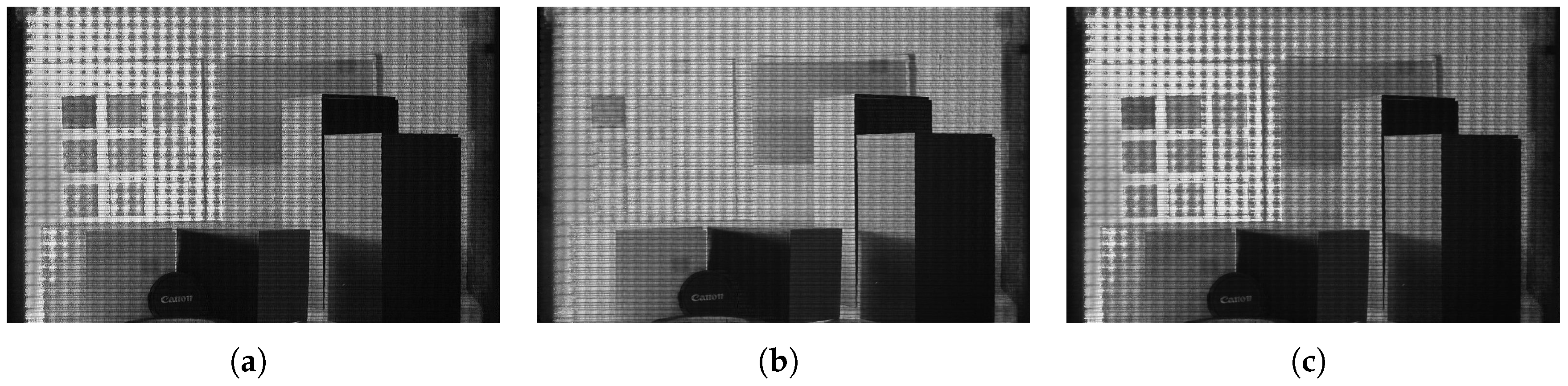
• Using as threshold the smaller mode and using as final value the mean of the remaining higher values (Figure 6a).
  

  Figure 6. Results obtained from methods based on mode + mean (a) only mode (b), and mean of mode (c).
• Using an arbitrary threshold and using as final value the mode of the remaining higher values (Figure 6b).
• Using an arbitrary threshold and using as final value the mean of two or more mode of the remaining higher values (Figure 6c).

As can be seen in Figure 6, none of these attempts led us to an acceptable result. At last, we changed our approach: to be sure not to include the mask in the final image, we tried to consider only the higher values in $F_{\mathrm{P}}$. Let’s call:

$$Q=\left\{uniqueorderedvaluesin{F}_{\mathrm{P}}\right\}$$

$$m_1=max\left(Q\right),m_2=max(Q-\left\{m_1\right\}),m_3=max(Q-\left\{m_1,m_2\right\});$$

$$Q_{\mathrm{M}}=\left\{m_1,m_2,m_3\right\}$$

$$M=\left[f\left(P_{\mathrm{I}}\right)in{F}_{\mathrm{P}}\left|f\right(P_{\mathrm{I}})\in Q_{\mathrm{M}}\right]$$

M is the set of the three highest different values assumed by the pixel (only if a pixel has more than two different values, that is cardinality $\#Q>2$; otherwise M contains all the values in $F_{\mathrm{P}}$). In the final reconstructed image, we use as value of every pixel $P_{\mathrm{I}}$ the mean of its set of values A. The result produced by this method can be observed in Figure 7a–c: the remaining horizontal noise is caused by the poor precision of the vertical movement of the grid. Considering for the reconstruction only the higher values of each pixel leads to a slightly brighter image; it can also add more noise to the reconstructed image if the lamp is not properly masked and some direct light reaches the occlusion mask during the acquisition phase (the noisy image reconstructed in this case can be seen in Figure 7d): this condition has obviously to be avoided regardless from the reconstruction method used.

Figure 7. (a–c) reconstruction of scene at EV 0, 2, −2; (d) noise produced by direct light on the grid.

4.3. The Algorithm

Summing up, here are presented the principal steps of the algorithm to produce the final image:

• Acquisition of an array of photos, to cover the entire scene with the holes of the occluding mask; this process is repeated for every exposure value of the final HDRI.
• For every exposure, reconstruction of the scene starting from the un-occluded zones of the mask.
• Assembling of the reconstructed images with different EV values, producing the final HDRI.

The final HDR image produced by this algorithm, confronted with the HDR image obtained without the occlusion mask method, is shown in Figure 8.

Figure 8. Comparison between two HDR captures, tone mapped for display purpose. (a) the veiling glare causes a loss of contrast, mostly in the darker regions; (b) reconstructed image as result of the method presented in this paper, described in Section 4.3.

The difference between our procedure and the one used by Talvala et al. [5] lies in the order of the operations: Talvala et al. [5] mounted an HDRI for each mask translation (step 3) and then reconstructed the final image (step 2). They also used planar homology considerations in phase of reconstruction, while we reasoned on the histogram of values assumed by each pixel in pictures with the same exposure.

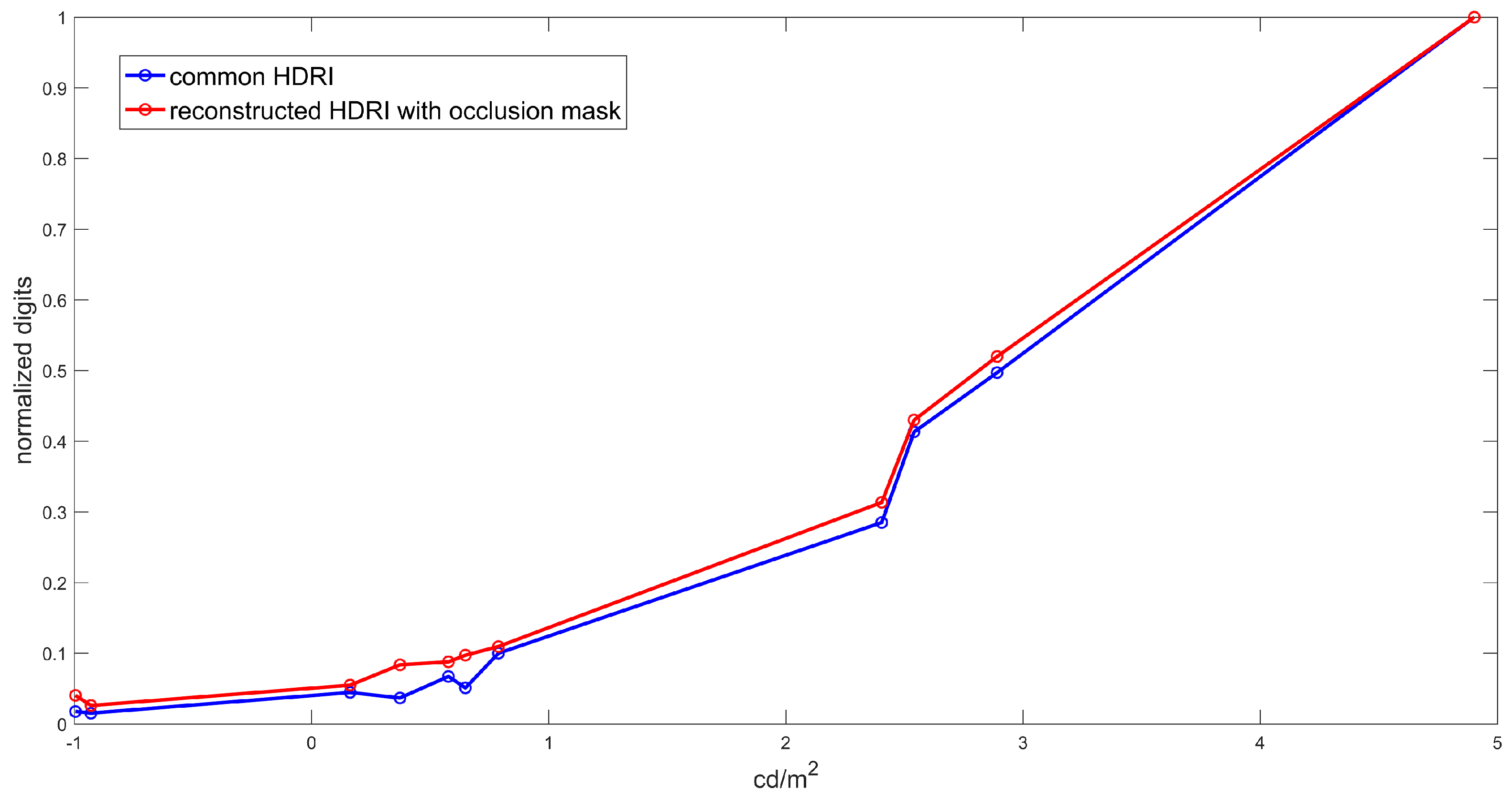
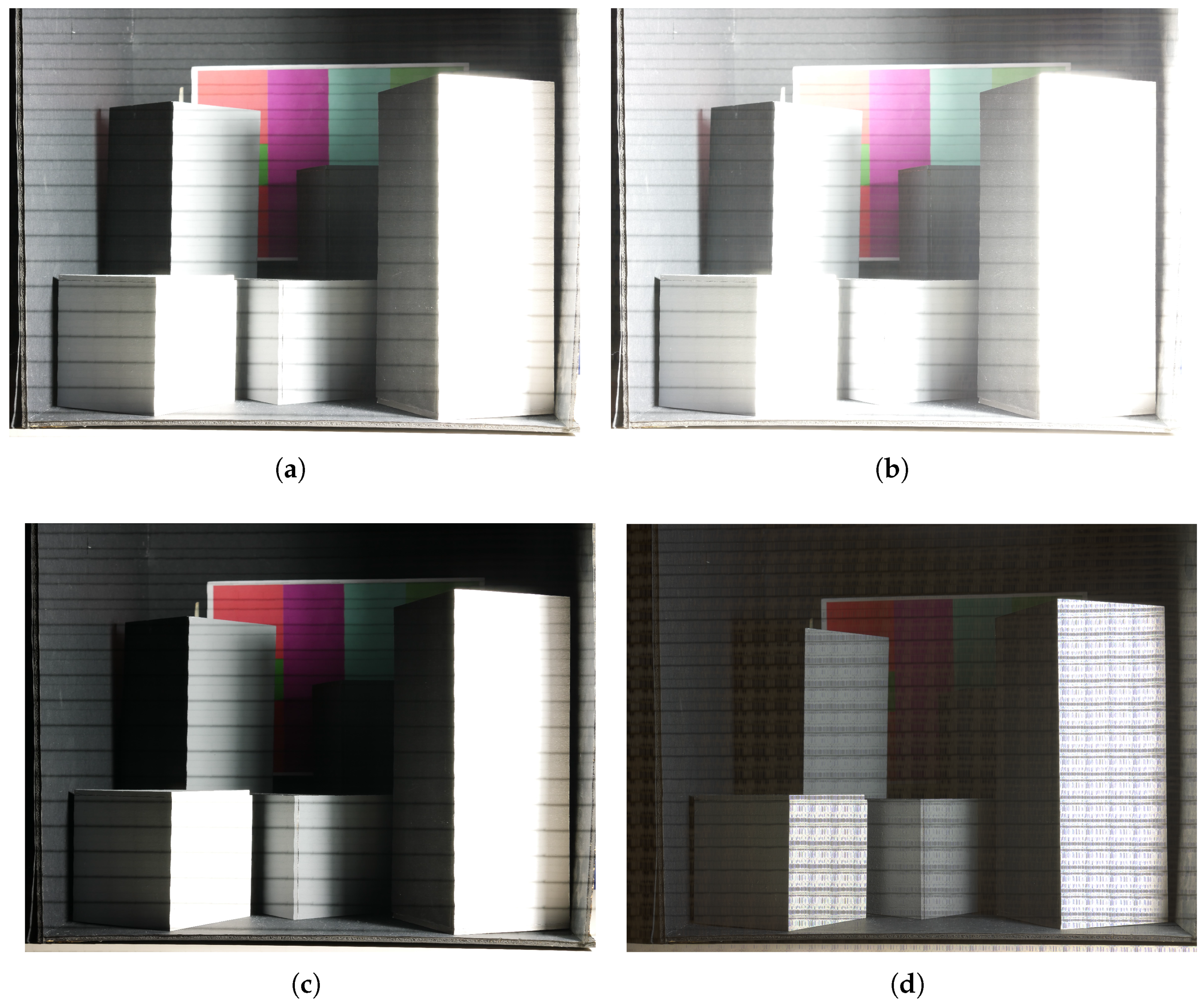
5. Results and Discussion

After the composition of the final HDR image we can see a visual improvement of the image quality: it appears clearer and less blurred comparing to both the HDRI with the original settings and an HDRI with the correct exposition.

The graph in Figure 9 shows the ratio between luminous intensity, measured in different points of the scene and the relative digit, normalized on the value of the most luminous point between the ones under consideration (not clipped). As we can see from the two curves, the one which represent the reconstructed HDR image is always under the other HDR image‘s curve, which is the one with the original settings. From that we can say this method reduces the amount of veiling glare in the scene.

Figure 9. Ratio between luminous intensity and its corresponding digit for both curves.

Furthermore, if we confront the two histograms, we can observe that the histogram of the reconstructed HDRI is more equalized. That confirms an improvement of the contrast and consequently of the the dynamic range.

Here we present a quantitative comparison between our method and the one proposed by Talvala et al. [5]. Glare and consequently its removal is image dependent, thus the presented comparison, done on different image sets, is mainly indicative. Talvala et al. [5] worked on a scene with a range of Luminance of 720:1 cd/m${}^2$, while we measured in our scene a range of Luminance of 1106:1 cd/m${}^2$. Regarding image dynamic range, Talvala et al. [5] could not estimate it in the whole scene after the process of reconstruction for the following reason: “At strong luminance edges where high-frequency glare is most apparent, we fail to recover scene content. Therefore, regions such as the top of the mirror or the blue egg become black after glare removal. Because of these artifacts, presenting whole-scene dynamic range figures would be inappropriate”. Then, they calculated the ratio of the values measured in some parts of the scene to the average value of the brightest zone (the background) before and after the reconstruction method. We calculated instead the dynamic range of the two HDR images, with the occlusion mask (after the reconstruction process) and without it. The data we collected are shown in Table 2.

Table 2. Comparison of dynamic ranges measured on the HDRI with and without the occlusion Mask.

Analysis	Without Occlusion Mask	With Occlusion Mask
Talvala et al. Object 1	560:1	22,400:1
Talvala et al. Object 2	505:1	8850:1
Cozzi et al. Whole Scene	603:1	1503:1

6. Conclusions

In conclusion, in this article we analysed the method of Talvala et al. [5] for the removing of the veiling glare in HDRI, and we proposed an algorithm based on the same occlusion mask, to study the benefits provided by it in HDRI acquisition process. Based on the results obtained, we can say that using an occlusion mask during the acquisition of the image causes a global reduction of the amount of glare in the image, even without making any estimate or subtraction. Limitations of our study are due to the large number of shots to reconstruct the whole scene in high precision, during the translation of grid, for getting low noise in the reconstruction process. A negative aspect of our reconstruction alghoritm is given by the use of the highest pixel values for each shoot taken with different shutter speeds so that the reconstructed HDRI is, on average, more luminous. In conclusion, we can say that veiling glare cannot be removed based only on data scene. We hope that in the future, we will propose new and alternative methods.

References

- Reinhard, E.; Ward, G.; Pattanaik, S.; Debevec, P. High Dynamic Range Imaging—Acquisition, Display and Image-Based Lighting; Morgan Kaufman Publishers: Burlington, MA, USA, 2006; pp. 142–149. [Google Scholar]
- Mccann, J.J.; Rizzi, A. Veiling glare: the dynamic range limit of HDR images. In Human Vision and Electronic Imaging; Spie, F., Ed.; International Society for Optics and Photonics: Bellingham, WA, USA, 2007; pp. 32–58. [Google Scholar]
- Boynton, P.A.; Kelly, E.F. Liquid-filled camera for the measurement of high-contrast images. Proc. SPIE 2003, 5080, 50–100. [Google Scholar]
- Starck, J.; Pantin, E.; Murtagh, F. Deconvolution in astronomy: A review. In Publications of the Astronomical Society of the Pacific; Astronomical Society of the Pacific: San Francisco, CA, USA, 2002; pp. 1051–1069. [Google Scholar]
- Talvala, E.V.; Adams, A.; Horowitz, M.; Levoy, M. Veiling Glare in High Dynamic Range Imaging. ACM Trans. Graph. 2007, 32–58. [Google Scholar] [CrossRef]
- Nayar, S.K.; Krishnan, G.; Grossberg, M.D.; Raskar, R. Fast separation of direct and global components of a scene using high frequency illumination. ACM Trans. Graph. 2006, 25, 935–944. [Google Scholar] [CrossRef]