Image Reconstruction with Reliability Assessment in Quantitative Photoacoustic Tomography

Abstract

Quantitative photoacoustic tomography is a novel imaging method which aims to reconstruct optical parameters of an imaged target based on initial pressure distribution, which can be obtained from ultrasound measurements. In this paper, a method for reconstructing the optical parameters in a Bayesian framework is presented. In addition, evaluating the credibility of the estimates is studied. Furthermore, a Bayesian approximation error method is utilized to compensate the modeling errors caused by coarse discretization of the forward model. The reconstruction method and the reliability of the credibility estimates are investigated with two-dimensional numerical simulations. The results suggest that the Bayesian approach can be used to obtain accurate estimates of the optical parameters and the credibility estimates of these parameters. Furthermore, the Bayesian approximation error method can be used to compensate for the modeling errors caused by a coarse discretization, which can be used to reduce the computational costs of the reconstruction procedure. In addition, taking the modeling errors into account can increase the reliability of the credibility estimates.

1. Introduction

Photoacoustic tomography (PAT) is a novel hybrid imaging modality developed during the past few decades [1]. In PAT, images of an initial pressure distribution caused by absorption of an externally introduced light pulse are reconstructed from photoacoustic measurements made on the boundary of the target. The method combines high contrast due to optical absorption and accurate resolution due to ultrasound propagation. The optical contrast is provided by absorption by different light absorbing molecules, chromophores. Chromophores of interest include, for example, haemoglobin, melanin, and various contrast agents [2]. PAT can be used to image biological tissues such as blood vessels and microvasculature of tumors in medical imaging and small animals in biomedical applications [3,4,5,6,7,8]. Furthermore, instrumentation is moderately simple and cheap, and there has been no reported evidence of health risks [4]. These properties make PAT attractive for medical imaging and biomedical studies.

In quantitative photoacoustic tomography (QPAT), one aims at estimating the absolute spatially varying concentrations of chromophores from photoacoustic images. Thus, it can be regarded as a second step after the conventional PAT. Sometimes, the conventional PAT is referred to as the acoustic inverse problem of QPAT and the following step, i.e., estimation of the optical parameters, is referred to as the optical inverse problem of QPAT [9]. QPAT is an ill-posed problem which needs to be approached in the framework of inverse problems. The ill-posedness means that even small errors in measurements or modeling can cause large errors into the reconstructions [10].

In QPAT, the distributions of the chromophore concentration can be estimated directly from the photoacoustic images obtained at multiple wavelengths, or first by reconstructing the absorption coefficients from photoacoustic images and then computing the concentrations utilizing the absorption spectra of known chromophores [9,11,12,13,14,15]. In addition to absorption, scattering effects need to be taken into account in order to obtain accurate results [12,16,17]. Estimation of more than one optical parameter in QPAT is, in general, a non-unique problem if only one illumination or wavelength is used [18,19]. To overcome the non-uniqueness, multiple illuminations [16,20,21,22,23] or wavelengths [11,12,13,15] can be used. Furthermore, combining QPAT with diffuse optical tomography has also been shown to improve the accuracy of the reconstructions [24,25,26,27]. Recently, one-step approaches in which the optical parameters are estimated directly from the photoacoustic time-series have been proposed [28,29,30,31,32,33].

In addition to quantitative estimates of the optical parameters, reliability of the these tomographic images is of interest. Especially in applications where illumination of the tissue is possible only from one side, for example imaging of skin, reliability of the estimates depends on the distance from the sensors [34]. Therefore, methods for evaluating the reliability of the estimated parameters are needed. However, evaluating the reliability of tomographic images obtained with PAT or QPAT has only been investigated in few recent studies [28,35,36].

In this paper, we consider estimating optical absorption and scattering from photoacoustic images. We assume that the initial pressure distribution has been reconstructed and that the Grüneisen parameter, which connects the initial pressure and absorbed optical energy density, is known. This inverse problem is approached in the framework of Bayesian inverse problems [10]. Thus, following the framework, all parameters are modeled as random variables which are characterized by their probability distributions. Combining the model describing physics of QPAT imaging situation, i.e., light propagation and absorption, together with measurements and probability distributions of prior information of the optical parameters, the posterior distribution can be formulated. The posterior distribution is the full solution of the inverse problem and basically it could be solved using Markov Chain Monte Carlo (MCMC) methods [10]. However, these methods are computationally prohibitively too expensive in large dimensional tomographic inverse problems, and thus, point estimates of the posterior distribution are computed. In this work we consider maximum a posteriori (MAP) estimate which leads to formulation of the image reconstruction problem as a minimization problem in which the squared norm between the data and forward model predictions together with an additive penalization term obtained by prior information are minimized. This minimization problem can be solved using methods of computational optimization. Furthermore, in this work, reliability of the estimated parameters are evaluated. These are based on forming a local Gaussian approximation of the posterior distribution and evaluating the reliability through credible intervals.

Iterative solving of a non-linear image reconstruction problem, such as computing the MAP estimate, requires repetitive solutions of the forward model. Due to the ill-posedness of the problem, an accurate model to describe light propagation and absorption is required. On the other hand, in practical tomographical applications, fast and efficient reconstruction methods are crucial. The radiative transfer equation (RTE) can be used to describe the light transport accurately in biological tissue [37]. However, it is computationally expensive. The most commonly used model in optical imaging is the diffusion approximation (DA) of the RTE [38]. The DA describes light propagation accurately relatively far from a light source and when scattering coefficient is significantly higher than absorption coefficient. In practice, the solution of the forward model is numerically approximated using a numerical method in a discretized basis, for example finite element (FE) method. If too sparse discretization of the model is used, it may cause significant modeling errors to the solution. On the other hand, sparse discretization would be favorable in the sense that the computation costs, for example memory usage and computation times, can be reduced. In this work, we consider QPAT in diffuse regime, i.e., highly scattering medium of size several millimeters, and use the DA as the model for light transport. In addition, modeling of approximation errors due to using coarse FE-discretization and its impact on both MAP estimates and credible intervals are studied through Bayesian framework.

In this work, Bayesian approximation error (BAE) modeling [10,39] is used for modeling of errors in QPAT. In the BAE modeling, systematic differences between accurate and inaccurate solutions (for example fine and coarse discretization) are approximated as a Gaussian random variables and this approximation is included into the solution of the inverse problem. Previously, BAE modeling has been utilized in QPAT in reduction of modeling errors caused by marginalization of scattering coefficient [17] and compensation of inaccuracies due to the numerical approximation of an acoustic solver [40]. In other optical and acoustic imaging modalities, BAE approach has been utilized, for example in diffuse optical tomography in model reduction [41,42,43,44], and compensating uncertainties in optode positions and boundary shape [45,46,47] and in full-waveform ultrasound tomography in compensating errors due to reduced discretization and approximate boundary models [48].

The rest of the paper is organized as follows. Forward model, inverse problem and BAE approach for QPAT are described in Section 2. In Section 3, numerical setup and methods are presented. Results are given in Section 4, and discussion and conclusions of the results are given in Section 5.

2. Materials and Methods

2.1. Forward Model

In QPAT, the tissue region of interest is illuminated by a short pulse of light. As light propagates within the tissue, it is absorbed by chromophores. This generates localized increases in pressure. This pressure increase propagates through the tissue as an acoustic wave and can be detected by ultrasound sensors on the boundary of the tissue. The propagation of the acoustic wave occurs approximately five orders of magnitude slower than propagation and absorption of light. Therefore, the total absorbed optical energy density is of interest and the rate of the absorption does not need to be modeled. Thus, in QPAT, light propagation can be modeled using a time-independent model of light transport. In this work, both Monte Carlo simulations [43,49,50] and the diffusion approximation [37] are used to model light propagation. The DA is of the form

$$\begin{array}{c}\hfill \left\{\begin{array}{cc}-\nabla ·\kappa (r)\nabla \mathsf{\Phi }(r)+{\mu }_a(r)\mathsf{\Phi }(r)\hfill & =0,r\in \mathsf{\Omega }\hfill \\ {\xi }_d\mathsf{\Phi }(r)+\frac{1}{2}A\kappa (r)\nabla \mathsf{\Phi }(r)·\nu \hfill & =\left\{\begin{array}{cc}s(r)\hfill & r\in ϵ\subset \partial \mathsf{\Omega }\hfill \\ 0\hfill & \mathrm{otherwise}\hfill \end{array}\right.\hfill \end{array}\right.\end{array}$$

(1)

where $\mathsf{\Phi }(r)$ is the photon fluence at spatial position r, $\kappa (r)={(d({\mu }_a(r)+{\mu }_s(r)(1-g)))}^{-1}$ is the optical diffusion coefficient, g is the mean of the cosine of the scattering angle, ${\mu }_a(r)$ is the optical absorption coefficient, ${\mu }_s(r)$ is the optical scattering coefficient, d is the dimension ($d=2,3$), ${\xi }_d$ is a dimension dependent scaling factor (${\xi }_2=1/\pi$ and ${\xi }_3=0.25$), $\nu$ is the outward boundary normal, A describes light reflectivity, $s(r)$ is the inward light current on the boundary $\partial \mathsf{\Omega }$ of the domain $\mathsf{\Omega }$, and $ϵ$ is the position of the light source. In this work, the solution of the DA (1) is numerically approximated using the Galerkin finite element method (FEM). Absorption, scattering and fluence are discretized using piecewise linear basis functions. For more detailed formulation of the FE approximation, see e.g., [16,17,28]. Furthermore, the absorbed optical energy density $H(r)$ is related to photon fluence by

$$H(r)={\mu }_a(r)\mathsf{\Phi }(r)$$

(2)

and the initial acoustic pressure $p_0(r)$ is

$$p_0(r)=G(r)H(r)$$

(3)

where $G(r)$ is the Grüneisen parameter which is used to identify photoacoustic efficiency [9]. The propagation of resulting photoacoustic wave can be modeled using equations of linear acoustics [51].

2.2. Inverse Problem

In this work, the inverse problem of QPAT, i.e., estimation of distributions of the optical parameters from photoacoustic images, is considered. We assume that the acoustic inverse problem is already solved and that the Grüneisen parameter is known, and thus, the data of the inverse problem is absorbed optical energy density. The acoustic inverse problem can be solved, for example, using backprojection method [52], methods based on eigenfunction expansion [53,54], time-reversal [55,56,57], penalized least squares [58,59,60,61] and Bayesian approach [35,36]. Let us denote the data vector by $y={[H_1,H_2,\dots ,H_M]}^{\mathrm{T}}\in {\mathbb{R}}^M$, where M is the number of data points, which is in this case is the number of illuminations multiplied with the number of nodes in FE-discretization that represent the data space. Further, let us denote the distribution of the optical parameters by $x(r)={[{\mu }_a(r),{\mu }_s(r)]}^{\mathrm{T}}$.

In the case of an additive noise model, an observation model for QPAT can be written as

$$y=f(x(r))+e,$$

(4)

where f is the forward model which maps the optical parameters to the data and $e\in {\mathbb{R}}^M$ denotes the noise. In practice, the observation model and the parameters are usually discretized as $f\mapsto f_h:{\mathbb{R}}^{2N}\mapsto {\mathbb{R}}^M$ and $x(r)\mapsto x\in {\mathbb{R}}^{2N}$, where h is the discretization parameter. Further, $x={[{\mu }_a,{\mu }_s]}^{\mathrm{T}}\in {\mathbb{R}}^{2N}$ denotes discretized parameters ${\mu }_a={[{\mu }_{a_1},{\mu }_{a_2},\dots ,{\mu }_{a_N}]}^{\mathrm{T}}\in {\mathbb{R}}^N$ and ${\mu }_s={[{\mu }_{s_1},{\mu }_{s_2},\dots ,{\mu }_{s_N}]}^{\mathrm{T}}\in {\mathbb{R}}^N$ where N is the number of FE nodes in the parameter grid. In this work, the discretized forward model $f_h(x)$ is based on the FE-approximation of the DA (1) and absorbed optical energy density (2). Discretized observation model is then

$$y=f_h(x)+e.$$

(5)

In the Bayesian approach [10], the variables x, y and e are considered as random variables. Solution of the inverse problem is the posterior probability density ${\pi }_{x|y}(x|y)$, which can be computed using Bayes’ formula as

$${\pi }_{x|y}(x|y)=\frac{{\pi }_x(x){\pi }_{y|x}(y|x)}{{\pi }_y(y)},$$

(6)

where ${\pi }_x(x)$ is the prior density, ${\pi }_{y|x}(y|x)$ is the likelihood density and ${\pi }_y(y)$ is the normalization constant. Prior density describes the beforehand information about the unknown x and likelihood density describes the likelihood of a specific measurement outcome with given parameters. Probability density ${\pi }_y(y)$ is constant for a given measurement, and therefore we can write the posterior as

$${\pi }_{x|y}(x|y)\propto {\pi }_x(x){\pi }_{y|x}(y|x).$$

(7)

Further, if x and e are uncorrelated, the posterior distribution can be written in the form

$${\pi }_{x|y}(x|y)\propto {\pi }_x(x){\pi }_e(y-f(x)),$$

(8)

where ${\pi }_e$ is the probability density of the noise e. In this work, distributions ${\pi }_x(x)$ and ${\pi }_e(e)$ are modeled as Gaussian distributions with

$$x\sim \mathcal{N}({\eta }_x,{\mathsf{\Gamma }}_x),e\sim \mathcal{N}({\eta }_e,{\mathsf{\Gamma }}_e),$$

where ${\eta }_x\in {\mathbb{R}}^{2N}$ and ${\eta }_e\in {\mathbb{R}}^M$ are the means and ${\mathsf{\Gamma }}_x\in {\mathbb{R}}^{2N\times 2N}$ and ${\mathsf{\Gamma }}_e\in {\mathbb{R}}^{M\times M}$ are the covariance matrices [10]. With these models, the posterior density can be written as

$${\pi }_{x|y}(x|y)\propto exp\left\{-\frac{1}{2}{(y-f_h(x)-{\eta }_e)}^{\mathrm{T}}{\mathsf{\Gamma }}_e^{-1}(y-f_h(x)-{\eta }_e)-\frac{1}{2}{(x-{\eta }_x)}^{\mathrm{T}}{\mathsf{\Gamma }}_x^{-1}(x-{\eta }_x)\right\}.$$

(9)

For more information on Bayesian approach to QPAT and modeling of noise, see e.g., [40].

As stated in Section 1, computing the full posterior distribution is typically computationally too expensive in practical tomographic imaging problems, and therefore, point estimates are considered. In this work, the MAP estimate is computed. It can be obtained by minimizing the negative of the exponent term of the posterior distribution

$$\begin{array}{cc}\hfill \widehat{x}& =\underset{x}{error}{\pi }_{x|y}(x|y)\hfill \\ & =\underset{x}{error}\left\{\frac{1}{2}{\left|\left|L_e(y-f_h(x)-{\eta }_e)\right|\right|}^2+\frac{1}{2}\Vert L_x(x-{\eta }_x){\Vert }^2\right\},\hfill \end{array}$$

(10)

where $\widehat{x}$ is the MAP estimate and ${\mathsf{\Gamma }}_x^{-1}=L_x^{\mathrm{T}}{L}_x$ and ${\mathsf{\Gamma }}_e^{-1}=L_e^{\mathrm{T}}{L}_e$ are the Cholesky decompositions of the inverse of the covariance matrices. In this work, we refer to the solution of (10) as the MAP estimate with the conventional error model.

2.3. Bayesian Approximation Error Modeling

Assume that the continuous model (4) can be approximated by a densely discretized finite-dimensional model

$$f_{\delta }:{\mathbb{R}}^{2N}\to {\mathbb{R}}^M,x\to f_{\delta }(x),\delta >0\mathrm{small}.$$

(11)

The discretized observation model, which is assumed to be numerically accurate within measurement precision, is of the form

$$y=f_{\delta }(x)+e.$$

(12)

In the Bayesian approximation error approach [10,39], the observation model is written in the form

$$\begin{array}{cc}\hfill y& =f_h(x)+(f_{\delta }(x)-f_h(x))+e\hfill \\ & =f_h(x)+\epsilon (x)+e.\hfill \end{array}$$

(13)

where $f_h(x)$ is the reduced model and $\epsilon (x)$ is the modeling error. The modeling error describes the discrepancy between the accurate forward model and the reduced model. The reduced model can be, for example, a model that is an approximation of the accurate physical model or a model with a coarse discretization. In the BAE modeling, the modeling error and the total error $n=\epsilon +e$ are approximated as Gaussian

$$\epsilon \sim \mathcal{N}({\eta }_{\epsilon },{\mathsf{\Gamma }}_{\epsilon }),n\sim \mathcal{N}({\eta }_n,{\mathsf{\Gamma }}_n),$$

where ${\eta }_n={\eta }_e+{\eta }_{\epsilon }$ and ${\mathsf{\Gamma }}_n={\mathsf{\Gamma }}_e+{\mathsf{\Gamma }}_{\epsilon }$. If the mutual dependence of x and $\epsilon$ is ignored, we get an approximation that is referred to as the enhanced error model [10] and the posterior density becomes

$${\pi }_{x|y}(x|y)\propto \left\{-\frac{1}{2}{(y-f_h(x)-{\eta }_n)}^{\mathrm{T}}{\mathsf{\Gamma }}_n^{-1}(y-f_h(x)-{\eta }_n)-\frac{1}{2}{(x-{\eta }_x)}^{\mathrm{T}}{\mathsf{\Gamma }}_x^{-1}(x-{\eta }_x)\right\}.$$

(14)

The MAP estimate using BAE is obtained as

$$\widehat{x}=\underset{x}{error}\left\{\Vert L_n{(y-f_h(x)-{\eta }_n)}^{\mathrm{T}}{\Vert }^2+\Vert L_x(x-{\eta }_x){\Vert }^2\right\},$$

(15)

where ${\mathsf{\Gamma }}_n^{-1}=L_n^{\mathrm{T}}{L}_n$. In this paper, we refer to the solution of (15) as the MAP estimate obtained with an enhanced error model.

In order to apply the approximation error statistics in the solution of the inverse problem, the statistics needs to be determined. In practice, the approximation error statistics can be approximated by investigating samples of the errors between an accurate model and a reduced model as follows [10,40]. First, a set of samples $\left\{x^{(\ell )},\ell =1,\dots ,L\right\}$ are drawn from the prior distribution of the optical parameters. Next, the forward problem is solved using the accurate and reduced models. Result is a set of forward solutions $\left\{f_{\delta }(x^{(\ell )})\right\}$ and $\left\{f_h(x^{(\ell )})\right\}$. Samples of the approximation error can then be computed as

$${\epsilon }^{(\ell )}=f_{\delta }(x^{(\ell )})-f_h(x^{(\ell )}),$$

(16)

and the mean and the covariance of the approximation error can be estimated as

$$\begin{array}{cc}\hfill {\eta }_{\epsilon }& =\frac{1}{L}\sum _{\ell =1}^L{\epsilon }^{(\ell )},\hfill \end{array}$$

(17)

$$\begin{array}{cc}\hfill {\mathsf{\Gamma }}_{\epsilon }& =\frac{1}{L-1}\sum _{\ell =1}^L{\epsilon }^{(\ell )}{{\epsilon }^{(\ell )}}^{\mathrm{T}}-{\eta }_{\epsilon }{\eta }_{\epsilon }^{\mathrm{T}}.\hfill \end{array}$$

(18)

Computing the approximation error statistics can be time consuming, but it is only required once per specific geometry and prior information. Thus, it can be done off-line before the measurements and image reconstruction.

2.4. Evaluating Credibility

In addition to point estimates for the unknown parameters, the Bayesian framework can be used to evaluate the reliability of the estimates. Credibility intervals would be the standard choice for the error estimates [39] but computing the intervals would again be computationally too expensive. In this paper, we approximate the posterior distribution as a locally Gaussian at the MAP estimate and evaluate the reliability similarly as in [28].

The forward model is approximated using the first order Taylor series

$$f(x)\approx f(\widehat{x})+J(\widehat{x})(x-\widehat{x}),$$

(19)

where $J(\widehat{x})$ is the Jacobian matrix of $f(x)$ evaluated at point $\widehat{x}$. By substituting the Taylor approximation into the observation model, a Gaussian approximation for the posterior distribution can be achieved

$$\pi (x|y)\sim \mathcal{N}(\widehat{\eta },\widehat{\mathsf{\Gamma }}),$$

(20)

where $\widehat{\eta }=\widehat{x}$ is the MAP estimate and

$$\widehat{\mathsf{\Gamma }}={(J{(\widehat{x})}^{\mathrm{T}}{\mathsf{\Gamma }}_e^{-1}J(\widehat{x})+{\mathsf{\Gamma }}_x^{-1})}^{-1}$$

(21)

is the covariance matrix.

For a Gaussian distribution, credibility intervals can be computed from the standard deviation (SD) of the distribution. For example, for a true Gaussian posterior distribution, the true value of the parameter $x_j$ lies in the interval $[{\eta }_{{\widehat{x}}_j}-3{\sigma }_{{\widehat{x}}_j},{\eta }_{{\widehat{x}}_j}+3{\sigma }_{{\widehat{x}}_j}]$, where ${\eta }_{{\widehat{x}}_j}$ and ${\sigma }_{{\widehat{x}}_j}$ are the mean and the standard deviation of ${\widehat{x}}_j$, with probability of $99.7\%$. In this work, we compute these credibility intervals $[{\eta }_{\widehat{x}}-p{\sigma }_{\widehat{x}},{\eta }_{\widehat{x}}+p{\sigma }_{\widehat{x}}]$ with different values of p. The standard deviation of the parameter ${\widehat{x}}_j$ is obtained from the diagonal values of the covariance matrix of the posterior approximation

$${\sigma }_{{\widehat{x}}_j}=\sqrt{\widehat{\mathsf{\Gamma }}(j,j)}.$$

(22)

3. Simulation Studies

Bayesian approach for image reconstruction and reliability estimation with and without discretization errors was studied with two-dimensional (2D) simulations. Compensation of the approximation errors through Bayesian approximation error modeling was studied. In the simulations, a rectangular domain of size 15 × 10 mm was considered. Two targets were investigated: (I) large smooth inclusions; and (II) blood-vessel-mimicking inclusions. In the simulations, absorption and scattering coefficients were chosen to be in the scale of the optical properties of fat tissue and blood [2,62,63]. Further, scattering anisotropy parameter of $g=0.8$ and light reflectivity $A=1$ were used.

3.1. Data Simulation

To simulate data, the domain was first illuminated by a planar illumination of uniform intensity covering one side of the rectangular domain. The photon fluence was simulated using a Monte Carlo method [43,49,50] in a piecewise constant triangular discretization ${\mathcal{H}}_s$. Then, the absorbed optical energy density was computed using Equation (2). To avoid making an inverse error, the simulated data was interpolated to the data space of the inverse problem which was piecewise linear representation of the absorbed optical energy density in a discretization ${\mathcal{H}}_h$. Random Gaussian noise was added to the simulated optical energy density data, with zero mean and standard deviation of 0.1 % of the maximum value of the simulated data. This process was repeated for all four sides of the domain each acting as light illumination side on their turn, resulting in four data vectors. The number of data obtained was then $4\times N_n$, where $N_n$ is the number of the nodes in the data space. Strength of the inward light source was set to 1 and the number of photon packets used in the simulations was ${10}^8$. The number of elements and nodes of the FE discretizations utilized in this study are given in

Table 1. FE discretizations used in the study: number of elements $N_e$ and number of nodes $N_n$.

	Mesh	${\mathit{N}}_{\mathit{e}}$	${\mathit{N}}_{\mathit{n}}$
Data simulation	${\mathcal{H}}_s$	104,472	52,654
Coarse mesh, basis for optical parameters	${\mathcal{H}}_h$	2052	1085
Fine mesh	${\mathcal{H}}_{\delta }$	32,832	16,649
Prior samples for evaluating the credibility	${\mathcal{H}}_b$	1932	1024

.

3.2. Inverse Problem

The inverse problem was solved using the methodology described in Section 2. Two discretizations for the representation of the fluence were considered: a fine mesh ${\mathcal{H}}_{\delta }$, which can be considered to be accurate, and a coarse mesh ${\mathcal{H}}_h$, which can be assumed to be too coarse to approximate light propagation accurately. The number of nodes and elements in these discretizations are given in Table 1. The unknown absorption and scattering parameters were presented in piecewise linear bases in ${\mathcal{H}}_h$. Two MAP estimates were studied: a MAP estimate with the conventional error model (MAP-CEM) which was obtained by minimizing (10) and a MAP estimate with the enhanced error model (MAP-EEM) which was obtained by minimizing (15). In both cases, the fluence was represented in a piecewise linear basis in the coarse discretization ${\mathcal{H}}_h$. For comparison, a MAP estimate with the conventional error model using a fine discretization for the fluence in the mesh ${\mathcal{H}}_{\delta }$ (MAP-REF) was solved. This can be considered as a reference of the best available solution. In all reconstructions, the noise was modeled as Gaussian distributed using the known noise level, i.e., with mean ${\eta }_e=0$ and constant standard deviation of $0.1\%$ of the maximum value of the full data vector.

The estimated parameters were scaled in the solution space to ensure the numerical stability of the reconstruction algorithm. Scaled parameters $\tilde{x}={[{\tilde{\mu }}_a,{\tilde{\mu }}_s]}^T$ were computed by

$${\tilde{\mu }}_a=\frac{{\mu }_a}{{\eta }_{{\mu }_a}},{\tilde{\mu }}_s=\frac{{\mu }_s}{{\eta }_{{\mu }_s}}.$$

where ${\eta }_{{\mu }_a}$ and ${\eta }_{{\mu }_s}$ are the means of the priors for the absorption and scattering, respectively.

The minimization problems (10) and (15) were solved by Gauss–Newton method. The solution was obtained by iterations

$${\tilde{x}}_{i+1}={\tilde{x}}_i+k{(J{({\tilde{x}}_i)}^{\mathrm{T}}{\mathsf{\Gamma }}_e^{-1}J({\tilde{x}}_i)+{\mathsf{\Gamma }}_x^{-1})}^{-1}(J{({\tilde{x}}_i)}^{\mathrm{T}}(y-f({\tilde{x}}_i)-{\eta }_e)-{\mathsf{\Gamma }}_x^{-1}(\tilde{x}-{\eta }_x)),$$

(23)

where ${\tilde{x}}_i$ is the scaled MAP estimate at iteration i, k is the step length parameter and $J({\tilde{x}}_i)$ is the scaled Jacobian matrix of the forward model at point ${\tilde{x}}_i$. In this work, the step length parameter k was chosen by a projected line-search algorithm ensuring the positivity of the estimated parameters. An initial value for the Gauss–Newton algorithm was chosen to be the mean of the prior. Solution was assumed to be converged, when the total change in the norm which was minimized was smaller than ${10}^{-3}$ in three consecutive iterations.

In order to evaluate the reliability of the reconstructed images, the credible intervals were approximated as described in Section 2.4. Thus, a local Gaussian approximation (20) for a linearized problem was considered in the position of the MAP estimate, and the approximation for the covariance was obtained by Equation (21). The standard deviations for the estimated parameters were obtained from the diagonal values of the posterior covariance matrix (22). These were then used to form the credible intervals.

3.3. Prior Model

In this work, Ornstein–Uhlenbeck prior model was used [64]. Ornstein–Uhlenbeck prior is a Gaussian distribution with the covariance matrix defined as

$${\mathsf{\Gamma }}_{\mu }={\sigma }_{\mu }^2\mathsf{\Xi },$$

(24)

where ${\sigma }_{\mu }$ is the standard deviation of the prior distribution and

$$\mathsf{\Xi }(i,j)=exp(-\Vert r_i-r_j\Vert /l)$$

(25)

is the unit covariance matrix describing the spatial correlation of the Gaussian random field, i and j denote the row and column indices of the matrix, $r_i$ and $r_j$ denotes the grid node coordinates and l is the characteristic length scale parameter. The length scale parameter can be chosen such that we assume significant correlation within distance l. Full prior model utilized in this work was then

$${\eta }_x=\left(\begin{array}{c}{\eta }_{{\mu }_a}\\ {\eta }_{{\mu }_s}\end{array}\right),{\mathsf{\Gamma }}_x=\left(\begin{array}{cc}{\mathsf{\Gamma }}_{{\mu }_a}& 0\\ 0& {\mathsf{\Gamma }}_{{\mu }_s}\end{array}\right).$$

In the reconstructions, absorption values of the target were assumed to be within the interval $[0,0.4]{\mathrm{mm}}^{-1}$. The mean of the prior distribution was chosen to be the mean of that interval, and the standard deviation was chosen such that the interval is within one standard deviation from the mean. For the scattering, values were assumed to be within the interval $[0,12]{\mathrm{mm}}^{-1}$, and the mean and the standard deviation were chosen similarly. The mean, standard deviation and characteristic length of the priors for the absorption and scattering used in this work are given in

Table 2. Prior parameters used in the simulations. l is the length scale parameter, ${\eta }_{{\mu }_a}$ is the mean of the absorption, ${\eta }_{{\mu }_s}$ is the mean of the scattering, ${\sigma }_{{\mu }_a}$ is the standard deviation of the absorption and ${\sigma }_{{\mu }_s}$ is the standard deviation of the scattering. Values given are for the non-scaled parameters, and the corresponding values for the (unitless) scaled parameters (utilized in reconstruction procedure) are given in parentheses.

	$\mathit{l}(\mathit{mm})$	${\mathit{\eta }}_{{\mathit{\mu }}_{\mathit{a}}}({\mathit{mm}}^{-1})$	${\mathit{\eta }}_{{\mathit{\mu }}_{\mathit{s}}}({\mathit{mm}}^{-1})$	${\mathit{\sigma }}_{{\mathit{\mu }}_{\mathit{a}}}({\mathit{mm}}^{-1})$	${\mathit{\sigma }}_{{\mathit{\mu }}_{\mathit{s}}}({\mathit{mm}}^{-1})$
Reconstructions	1.25	0.2 (1)	6 (1)	0.2 (1)	6 (1)
Approximation error statistics	1.25	0.2	6	0.067	2
Reliability of the credibility intervals	1.25	0.2	6	0.067	2

.

3.4. Approximation Error Statistics

The statistics of approximation error was computed as described in Section 2.3. 10,000 samples $\{x^{(\ell )}\}$ were drawn from the prior distributions for absorption and scattering with prior parameters described in Table 2. In case of negative parameters were drawn, they were set to the value ${10}^{-6}$ in order to keep the model physical. Solution of the forward model, i.e., the FE-approximation of the DA was computed using fine and coarse meshes (${\mathcal{H}}_{\delta }$ and ${\mathcal{H}}_h$, respectively), resulting in fluences $\left\{{\mathsf{\Phi }}_{\delta }(x^{(\ell )})\right\}$ and $\left\{{\mathsf{\Phi }}_h(x^{(\ell )})\right\}$, respectively. Absorbed optical energies $\left\{H_{\delta }(x^{(\ell )})\right\}$ and $\left\{H_h(x^{(\ell )})\right\}$ were computed using Equation (2). Samples of the approximation error were computed from (16) using these absorbed optical energy densities, and the mean and the covariance of the approximation error were computed using (17) and (18).

3.5. Reliability of the Credibility Intervals

In order to investigate the effect of the Bayesian approximation error modeling on the credibility intervals, the Gaussian approximations of the posterior distributions were compared to the true Gaussian distribution. This was done as follow. First, a set of 400 samples of optical parameter distributions $\{x^{(q)},q=1,\dots ,Q\}$ were drawn from the prior distributions with parameters given in Table 2 using mesh ${\mathcal{H}}_b$. Then, these parameters were interpolated to the piecewise constant basis ${\mathcal{H}}_s$ in which Monte Carlo method was used to simulate data. In Monte Carlo simulations, ${10}^8$ photon packets were used for each illumination. The simulated data was interpolated to the piecewise linear data space in discretization ${\mathcal{H}}_h$, which was also used to present the optical parameters. Uncorrelated noise with zero mean and standard deviation of $0.1\%$ of the maximum value of the data was added to the data. Then, MAP-CEM and MAP-EEM estimates and approximations of the posterior distribution were computed in mesh ${\mathcal{H}}_h$ similarly as earlier using the known noise statistics and previously defined statistics for the approximation error model.

The amount of true optical parameters within the credibility intervals were computed for each of the reconstructions as follows. Let ${\widehat{\mu }}_{a_i}^{(q)}$ and ${\widehat{\mu }}_{s_i}^{(q)}$ be the estimated absorption and scattering of the sample q in node i. Further, let ${\mu }_{a_i}^{(q)}$ and ${\mu }_{s_i}^{(q)}$ be the true values of absorption and scattering of the sample q in node i, respectively. For each node, the percentage of the true values which lie in the interval $[\widehat{\mu }-{\sigma }_{\widehat{\mu }},\widehat{\mu }+{\sigma }_{\widehat{\mu }}]$ and $[\widehat{\mu }-3{\sigma }_{\widehat{\mu }},\widehat{\mu }+3{\sigma }_{\widehat{\mu }}]$ in the reconstructions were computed. For the absorption, this can be computed as

$${\mathcal{P}}_p(i)=\frac{1}{Q}\sum _{q=1}^Q{𝟙}_{\{{\widehat{\mu }}_{a_i}^{(q)}-p{\sigma }_{{\widehat{\mu }}_{a_i}}^{(q)}\le {\mu }_{a_i}^{(q)}\le {\widehat{\mu }}_{a_i}^{(q)}+p{\sigma }_{{\widehat{\mu }}_{a_i}}^{(q)}\}}·100\%,$$

(26)

where i is the index of the node, $p=1,3$, and $𝟙$ is the indicator function

$${𝟙}_{\{{\widehat{\mu }}_{a_i}^{(q)}-p{\sigma }_{{\widehat{\mu }}_{a_i}}^{(q)}\le {\mu }_{a_i}^{(q)}\le {\widehat{\mu }}_{a_i}^{(q)}+p{\sigma }_{{\widehat{\mu }}_{a_i}}^{(q)}\}}=\left\{\begin{array}{cc}1\hfill & {\widehat{\mu }}_{a_i}^{(q)}-p{\sigma }_{{\widehat{\mu }}_{a_i}}^{(q)}\le {\mu }_{a_i}^{(q)}\le {\widehat{\mu }}_{a_i}^{(q)}+p{\sigma }_{{\widehat{\mu }}_{a_i}}^{(q)}\hfill \\ 0\hfill & \mathrm{otherwise}\hfill \end{array}\right..$$

(27)

For the scattering, this can be computed similarly. These values can be compared to the true Gaussian distribution, in which the corresponding percentages are $68.2\%$ and $99.7\%$, respectively. For more studies of the feasibility of this approach, see [28].

4. Results

Results were compared visually and by computing relative errors of the estimated parameters by

$$E_{{\mu }_a}=100\%·\frac{\Vert {\widehat{\mu }}_a-{\mu }_a\Vert }{\Vert {\mu }_a\Vert },E_{{\mu }_s}=100\%·\frac{\Vert {\widehat{\mu }}_s-{\mu }_s\Vert }{\Vert {\mu }_s\Vert },$$

where the norm is Euclidean norm. Further, computation times were compared. The simulations were performed in MATLAB (R2016b, The MathWorks Inc., Natick, MA, USA). The reconstruction algorithm utilized in this work was not optimized, and therefore the computation times should be considered only as a qualitative comparison.

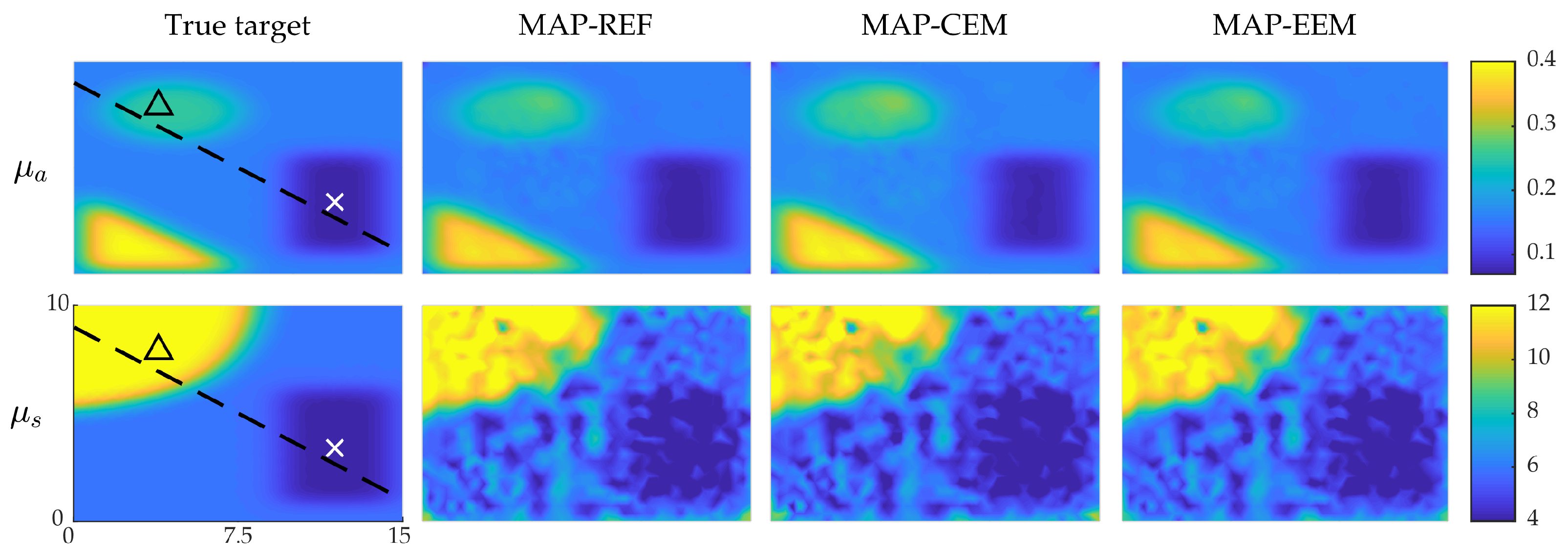
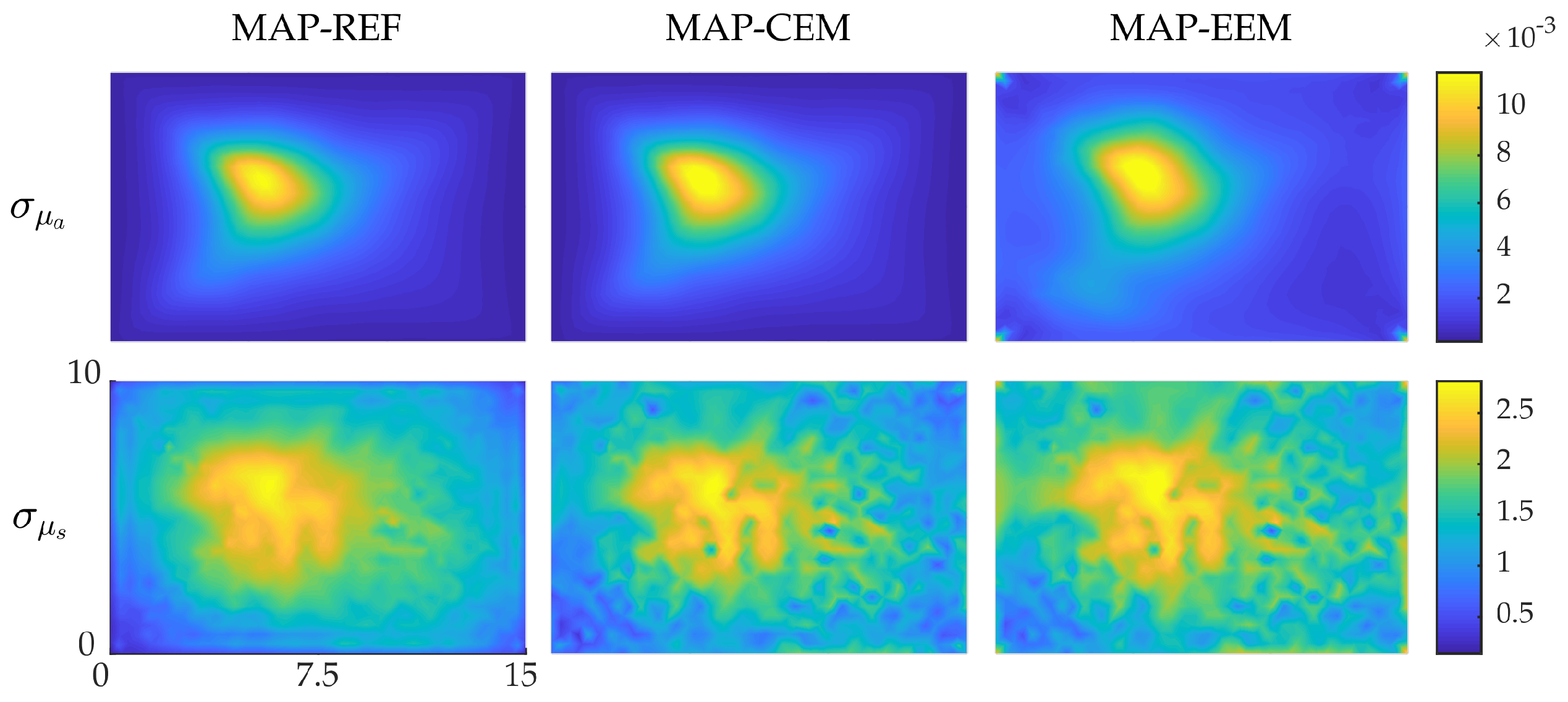
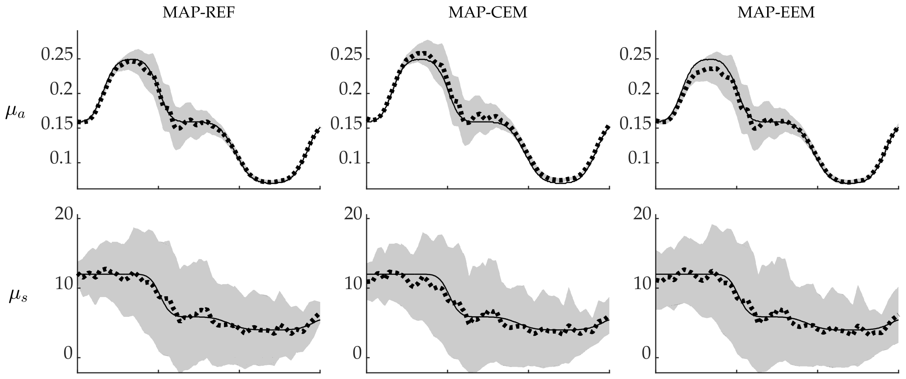
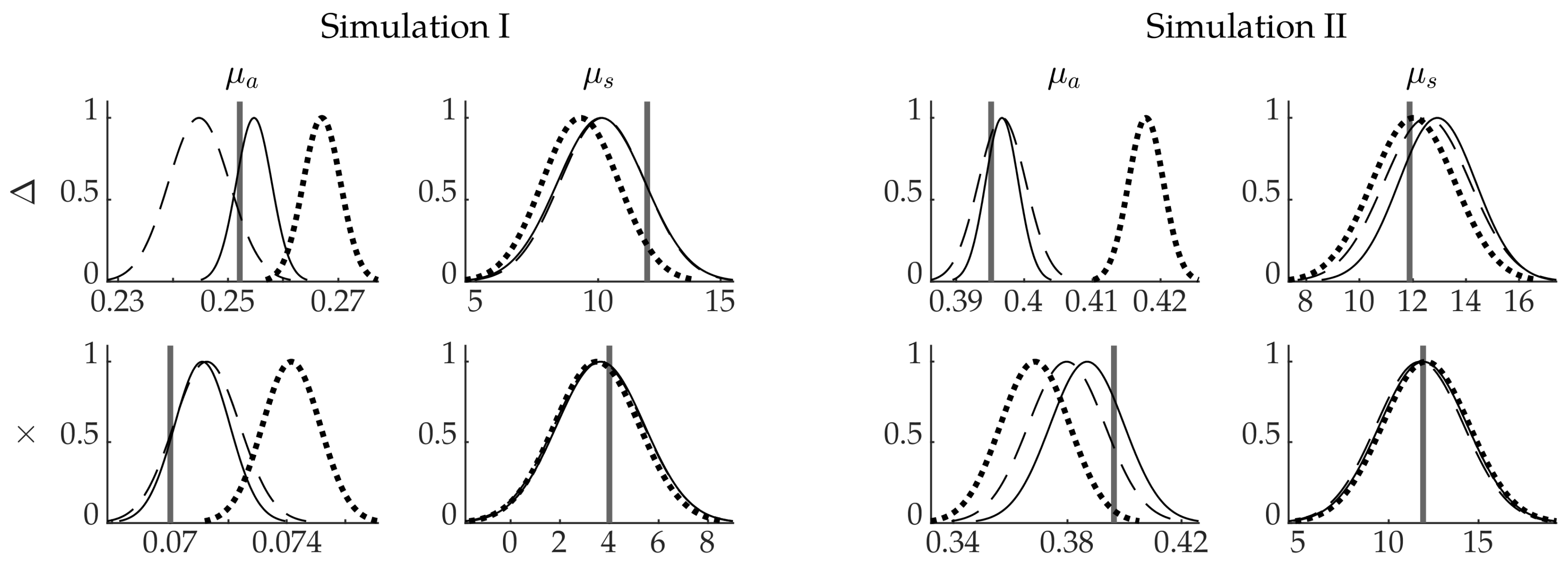
4.1. Simulation I: Smooth Inclusions

The simulated (true) optical parameters and the MAP estimates obtained with conventional error model in the fine discretization (MAP-REF) and coarse discretization (MAP-CEM) and enhanced error model (MAP-EEM) are shown in Figure 1. Visually inspecting it seems that there are no large differences between the absorption and scattering estimates obtained with different approaches. The absorption estimates are qualitatively better and the reconstructed inclusions resemble the original targets, whereas the scattering estimates suffer from artefacts. This difference in quality of absorption and scattering estimates is typical for QPAT and most likely due to more severe ill-posedness of the scattering estimation problem. It has also been noticed in other studies [11,21,40,65]. However, looking at the MAP-CEM estimate, the absorption estimates differ from the other estimates and the true values slightly. This is especially evident in the location of the highly absorbing inclusion in the top left corner of the domain. These differences can also be noticed in the relative errors of the estimates which are presented in

Table 3. Relative errors of the MAP-REF, MAP-CEM and MAP-EEM reconstructions compared to the true values. $E_{{\mu }_a}$ is the relative error of the absorption coefficient and $E_{{\mu }_s}$ is the relative error of the scattering coefficient.

	MAP-REF		MAP-CEM		MAP-EEM
	${\mathit{E}}_{{\mathit{\mu }}_{\mathit{a}}}$ (%)	${\mathit{E}}_{{\mathit{\mu }}_{\mathit{s}}}$ (%)	${\mathit{E}}_{{\mathit{\mu }}_{\mathit{a}}}$ (%)	${\mathit{E}}_{{\mathit{\mu }}_{\mathit{s}}}$ (%)	${\mathit{E}}_{{\mathit{\mu }}_{\mathit{a}}}$ (%)	${\mathit{E}}_{{\mathit{\mu }}_{\mathit{s}}}$ (%)
Simulation I	3.6	11.0	5.1	12.5	3.7	11.1
Simulation II	6.7	15.2	9.5	16.5	7.6	15.7

.

The standard deviations of the posterior distributions are shown in Figure 2. In all approaches, the SDs are larger in the interior of the domain where the photon fluence and absorbed optical energy density are weakest. Thus, the MAP estimates within those regions can be considered to be less reliable than the MAP estimates closer to the boundaries of the target. When comparing the SDs of the different approaches, it can be noticed that the estimates obtained using the conventional error model in the fine and the coarse mesh resemble each other. However, the SDs obtained using the enhanced error model in the coarse mesh are slightly larger especially close to the boundaries of the domain. Thus, in the case of the conventional error model, the obtained standard deviations are small for the fine mesh and the coarse mesh, although, the MAP estimates are not equally accurate. Utilizing the enhanced error model increases the standard deviations which indicates that they can be regarded as more realistic in this case.

The MAP-estimates with credible intervals along the cross-section through the domain (black dashed line in Figure 1) are shown in Figure 3. Here the differences between the MAP-CEM and MAP-EEM reconstructions can be seen more clearly. The MAP-CEM absorption estimates are larger than the true values in most of the locations, and most of the true values do not lie within the credibility intervals. On the other hand, the MAP-EEM estimates are closer to the true values and the MAP-REF estimates in most of the locations, although in the position of the inclusion with high absorption (left side of the cross-section) the MAP-CEM estimates seem to be closer to the true values than the MAP-REF and MAP-EEM estimates.

Marginal densities of the posterior distributions in two points inside the domain are presented in Figure 4 in the first and second column. Points are marked with × and △ in Figure 1. When looking at the absorption estimates, it can be noticed that the MAP-EEM estimates are closer to the true target values when compared to the MAP-CEM estimate. Higher uncertainty of the MAP-EEM absorption estimates can also be seen. The posterior approximations of the scattering are very similar. However, in the point within highly scattering and absorbing region close to the boundary (point △), there is a difference in the MAP-CEM and MAP-EEM estimates and posterior approximations of scattering, and the MAP-EEM estimate is closer to the true value than the MAP-CEM estimate.

Computation times in seconds for Gauss–Newton algorithm in MAP-REF, MAP-CEM, and MAP-EEM reconstructions are presented on the first row of

Table 4. Computation times in seconds and iterations done before the solution was converged for the Gauss–Newton algorithm for MAP-REF, MAP-CEM and MAP-EEM reconstructions for Simulation I (first row) and Simulation II (second row).

	MAP-REF		MAP-CEM		MAP-EEM
	Time (s)	Iteration	Time (s)	Iteration	Time (s)	Iteration
Simulation I	18,081	9	445	11	296	10
Simulation II	22,480	10	507	12	337	11

. The number of iterations in which the solutions converged varied, but computing the estimates in the coarse mesh clearly required significantly less computational effort compared to the fine mesh.

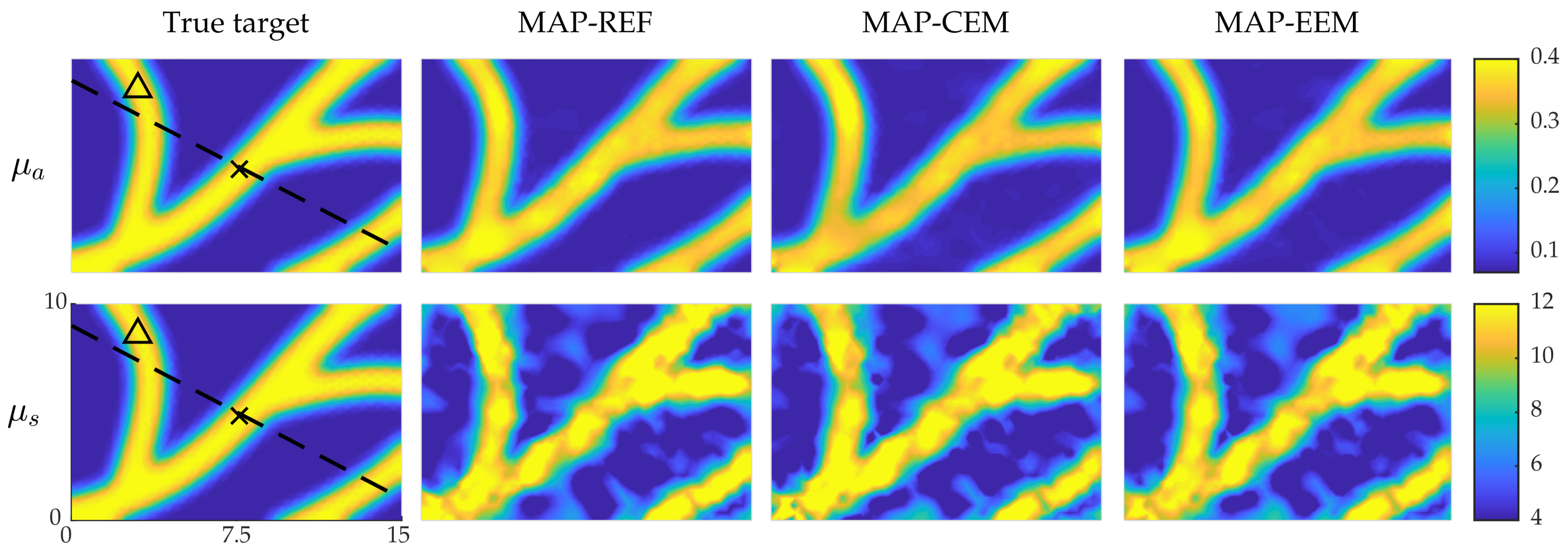
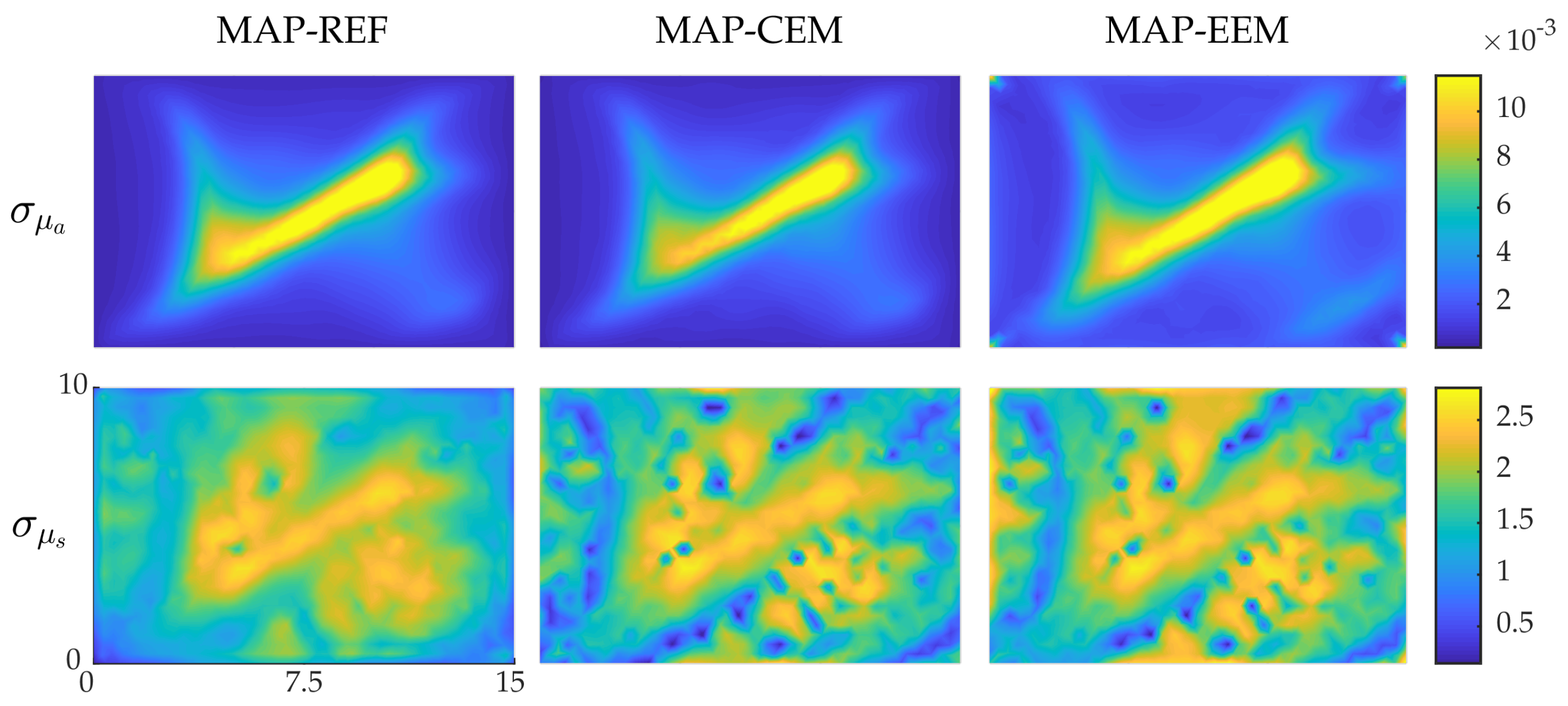
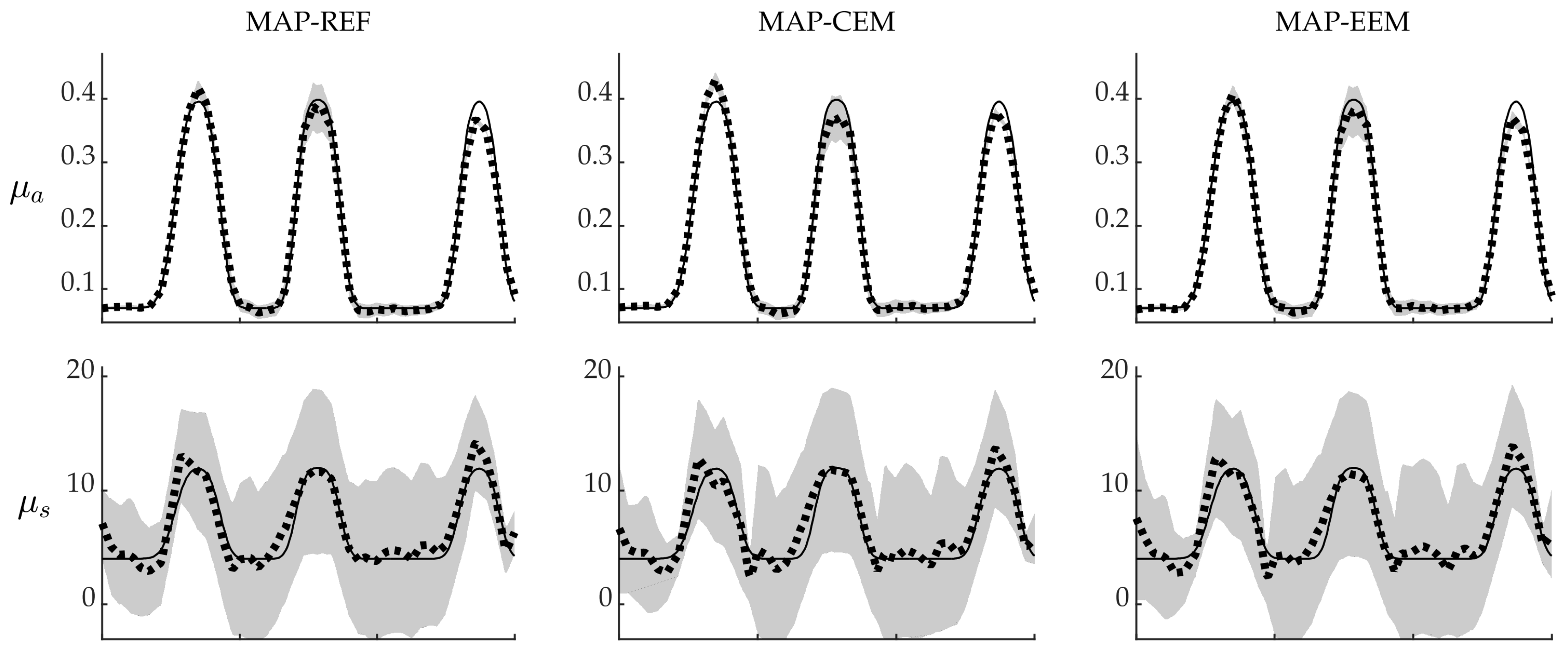
4.2. Simulation II: Blood-Vessel-Mimicking Inclusions

The simulated optical parameters and the MAP estimates obtained with conventional error model (MAP-REF and MAP-CEM) and enhanced error model (MAP-EEM) are shown in Figure 5. Similarly to the previous simulation, by visual inspection there are no large differences between the estimates, and the absorption estimates are qualitatively better than the scattering estimates. Differences between the the reconstructions can be seen more clearly in the relative errors, which are presented in Table 3.

Standard deviations of the reconstructions are shown in the Figure 6. Again, the SDs are larger in the interior of the domain. Furthermore, when compared with each other, the SDs of the MAP-REF and MAP-CEM estimates resemble each other, whereas SDs of the MAP-EEM estimates are slightly larger especially near the boundaries.

MAP estimates with credibility intervals along the cross-section through the domain are shown in Figure 7. As it can be seen, the absorption MAP-EEM estimates resemble the MAP-REF estimates more than the MAP-CEM estimates, especially on the left part of the cross-section. However, although the SDs are larger, the credibility intervals of the absorption are not reliable in the whole domain even for MAP-REF estimates. The credibility intervals of the MAP-EEM estimates are wider than MAP-REF or MAP-CEM estimates, but still the true values do not lie in the credibility intervals in the whole domain. Similar results can be observed in the scattering estimates to a lesser extent.

Marginal densities of the posterior distributions in two points inside the domain are presented in Figure 4 in the third and fourth column. In the absorption estimates, it can be seen that the MAP-EEM estimate is closer to the true value than the MAP-CEM estimate. Similarly, in the scattering, the MAP-EEM estimates are closer to the true value than the MAP-CEM estimates, but the differences are smaller than in the case of absorption. Higher standard deviations of the MAP-EEM estimates are also visible, especially in the absorption estimates in the point △.

Computation times in seconds for Gauss–Newton algorithm in the MAP-REF, MAP-CEM, and MAP-EEM reconstructions are presented in the second row of Table 4. Similarly to the Simulation I, computing the estimates in the coarse mesh required a significantly less computational effort compared to the fine mesh.

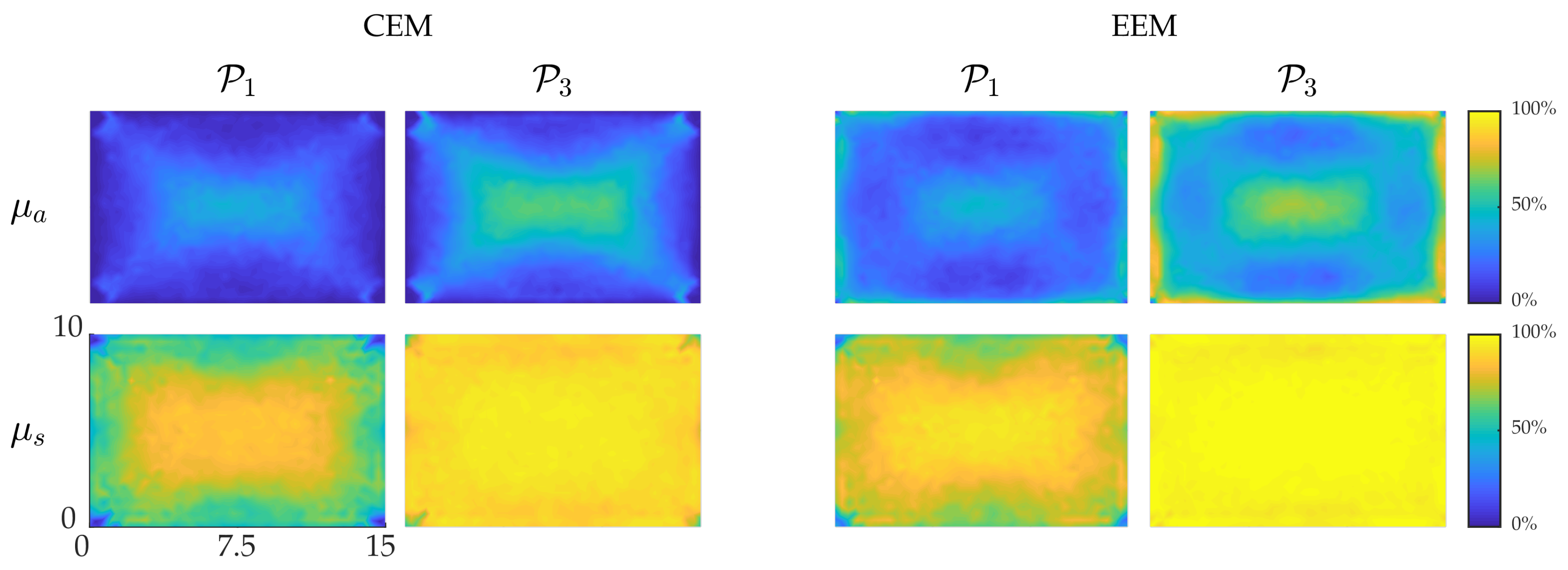
4.3. Reliability of the Credibility Intervals

Percentages of the true values of the parameters in each node which lie inside the credibility intervals $[\widehat{\mu }-{\sigma }_{\widehat{\mu }},\widehat{\mu }+{\sigma }_{\widehat{\mu }}]$ and $[\widehat{\mu }-3{\sigma }_{\widehat{\mu }},\widehat{\mu }+3{\sigma }_{\widehat{\mu }}]$ were visualized and are shown in Figure 8. For the MAP-CEM absorption reconstructions, the credibility intervals are narrow, especially near the boundary of the domain. Near the center of the domain, the bounds are closer to the true Gaussian values of $68.2\%$ and $99.7\%$. For the MAP-EEM absorption reconstructions, the percentages are larger, and especially near the boundaries the percentages are very close to the true Gaussian values. This indicates that using the enhanced error model increases the reliability of the credibility intervals. For the scattering, the percentages of the true values of the parameters in each node which lie inside the credibility intervals $[\widehat{\mu }-{\sigma }_{\widehat{\mu }},\widehat{\mu }+{\sigma }_{\widehat{\mu }}]$ and $[\widehat{\mu }-3{\sigma }_{\widehat{\mu }},\widehat{\mu }+3{\sigma }_{\widehat{\mu }}]$ are similar for both MAP-CEM and MAP-EEM reconstructions. However, in the MAP-EEM estimates, the values of ${\mathcal{P}}_1$ and ${\mathcal{P}}_3$ are closer to the Gaussian reference values.

5. Discussion and Conclusions

As seen in the simulations, estimates obtained utilizing the Bayesian approximation error method (MAP-EEM) are more accurate than estimates obtained by conventional noise model (MAP-CEM) when comparing them visually or by relative errors computed against the true target. Modeling errors caused by the coarse discretization are mostly due to the fast decrease of the photon fluence when distance to the light source increases. This change resembles exponential decay, which the coarse discretization is unable to present accurately. Although MAP-EEM estimates are not as accurate as the reference estimates computed with the fine discretizations (MAP-REF), computation cost was significantly reduced by utilizing the enhanced error model and coarse discretization.

Absorbed optical energy density, which was used as the data for the inverse problem, is the product of photon fluence and absorption coefficient. This causes the absorption to effect the data more than the scattering. This leads to more accurate estimates of the absorption compared to the scattering. This can also be seen in the posterior approximations: posterior of the absorption was significantly narrower, indicating that the estimates are more reliable than the scattering estimates.

In addition to providing more accurate estimates, standard deviation of the MAP-EEM estimates were larger compared to the MAP-CEM estimates, and thus, the credibility intervals were wider. Enhanced error model can be used to provide more reliable credibility estimates, which was observed when the statistics of the posterior approximation were compared to the true Gaussian values. The shape of the standard deviation distributions seemed to correlate with the distributions of the estimated parameters. This is caused by the fact that the posterior approximation is computed using the MAP estimate. Comparison between the approximation and the true posterior distribution could be done, but it would require computationally expensive methods, such as Markov chain Monte Carlo methods. Therefore more research would be required to study the validity of the Gaussian approximation of the posterior distribution.

Even though the inclusions in the simulations were smooth, the prior model utilized in this work does not represent the inclusions accurately especially in the case of the blood-vessel-mimicking inclusions. Still, accurate reconstructions could be achieved with this model. Samples for computing the statistics of the Bayesian approximation method and analyzing the reliability of the credible intervals were drawn from prior distribution with lower standard deviation than the prior distribution utilized in the reconstruction algorithm. High SD of the prior may generate absorption distributions with significantly higher values compared to the simulated inclusions, which may cause unrealistically large absorption close to the boundaries and weaken the photoacoustic signal from the central parts of the domain. Also, in case the approximation errors between the accurate and reduced model are too large, they cannot be approximated by a Gaussian distribution accurately [44]. The optimal prior distribution for the BAE statistics was not investigated in this work, and would require additional research.

The structures of the inclusion considered in the simulations were simple. Especially the blood-vessel-mimicking inclusions were too coarse to represent realistic blood vessels found in biological tissues. Reconstructing more complex structures necessitates on usage of finer discretization of the parameters, which decreases the modeling errors caused by the discretizations but increases computational burden. Further, the domain utilized in this work was large enough that the DA could be used to obtain accurate reconstructions from the data simulated with a Monte Carlo method. Considering realistic applications, the target may be smaller, and thus, the DA may not be a valid approximation and the RTE should be used as the light transport model. These could suggest a need for further development of methods for model reduction in QPAT.

In the simulations, the realization of the random measurement noise affected the overall accuracy of the estimates (results not shown ), i.e., the relative errors of the reconstructions varied depending on the realization of the noise. However, the general results remained unaffected. This was caused by the fact that the standard deviation of the random noise was proportional to the maximum value of the signal, which leads to a very low signal-to-noise ratio near the center of the domain. Furthermore, additive random noise was introduced to the measurement data due to the stochastic nature of the Monte Carlo method utilized in the data simulation. In order to minimize the amount of this stochastic Monte Carlo related noise, a large amount of photon packets was used in each simulation and thus, amount of this noise could be assumed to be small compared to the additive random noise.

The reconstruction problem considered in this work is only a part of the process required to obtain quantitative photoacoustic images in practical applications. In practice, first step would be the reconstruction of the initial pressure distribution and computing the absorbed energy density distribution from the photoacoustic signal measured from the surface. Furthermore, in this work the domain was illuminated from all sides, which may not be possible in clinical applications and could affect the accuracy of the reconstructions, especially far away from the light source. In that situation, reliable credibility estimates would be necessary when interpreting the reconstructions.

In conclusion, the Bayesian framework can be utilized to provide accurate estimates of the optical parameters and a method to assess the reliability of the estimates in the inverse problem of QPAT. Moreover, Bayesian approximation error method can be utilized to alleviate the modeling errors caused by a coarse discretization of the photon fluence. This can be utilized in the model reduction of the inverse problem. Furthermore, modeling of the errors can increase the reliability of the credibility estimates.

References

1. Xia, J.; Yao, J.; Wang, L.V. Photoacoustic tomography: Principles and advances. Electromagn. Waves 2014, 147, 1–22. [Google Scholar] [CrossRef]
2. Jacques, S.L. Optical properties of biological tissues: A review. Phys. Med. Biol. 2013, 58, R37–R61. [Google Scholar] [CrossRef]
3. Beard, P. Biomedical photoacoustic imaging. Interface Focus 2011, 1, 602–631. [Google Scholar] [CrossRef] [Green Version]
4. Wang, L.V. (Ed.) Photoacoustic Imaging and Spectroscopy; CRC Press: Boca Raton, FL, USA, 2009. [Google Scholar]
5. Xu, M.; Wang, L.V. Photoacoustic imaging in biomedicine. Rev. Sci. Instrum. 2006, 77, 041101. [Google Scholar] [CrossRef] [Green Version]
6. Li, C.; Wang, L.V. Photoacoustic tomography and sensing in biomedicine. Phys. Med. Biol. 2009, 54, R59–R97. [Google Scholar] [CrossRef]
7. Wang, L.V. Prospects of photoacoustic tomography. Med. Phys. 2008, 35, 5758–5767. [Google Scholar] [CrossRef] [Green Version]
8. Yao, J.; Xia, J.; Maslov, K.I.; Nasiriavanaki, M.; Tsytsarev, V.; Demchenko, A.V.; Wang, L.V. Noninvasive photoacoustic computed tomography of mouse brain metabolism in vivo. Neuroimage 2013, 64, 257–266. [Google Scholar] [CrossRef] [Green Version]
9. Cox, B.; Laufer, J.G.; Arridge, S.R.; Beard, P.C. Quantitative spectroscopic photoacoustic imaging: A review. J. Biomed. Opt. 2012, 17, 061202. [Google Scholar] [CrossRef]
10. Kaipio, J.; Somersalo, E. Statistical and Computational Inverse Problems; Springer: New York, NY, USA, 2005. [Google Scholar]
11. Pulkkinen, A.; Cox, B.T.; Arridge, S.R.; Kaipio, J.P.; Tarvainen, T. A Bayesian approach to spectral quantitative photoacoustic tomography. Inverse Probl. 2014, 30, 065012. [Google Scholar] [CrossRef]
12. Bal, G.; Ren, K. On multi-spectral quantitative photoacoustic tomography in a diffusive regime. Inverse Probl. 2012, 28, 025010. [Google Scholar] [CrossRef]
13. Cox, B.T.; Arridge, S.R.; Beard, P.C. Estimating chromophore distributions from multiwavelength photoacoustic images. J. Opt. Soc. Am. A 2009, 26, 443–455. [Google Scholar] [CrossRef]
14. Laufer, J.; Cox, B.; Zhang, E.; Beard, P. Quantitative determination of chromophore concentrations form 2D photoacoustic images using a nonlinear model-based inversion scheme. Appl. Opt. 2010, 49, 1219–1233. [Google Scholar] [CrossRef]
15. Razansky, D.; Baeten, J.; Ntziachristos, V. Sensitivity of molecular target detection by multispectral optoacoustic tomography (MSOT). Med. Phys. 2009, 36, 939–945. [Google Scholar] [CrossRef]
16. Tarvainen, T.; Cox, B.T.; Kaipio, J.P.; Arridge, S.R. Reconstructing absorption and scattering distributions in quantitative photoacoustic tomography. Inverse Probl. 2012, 28, 084009. [Google Scholar] [CrossRef]
17. Pulkkinen, A.; Kolehmainen, V.; Kaipio, J.P.; Cox, B.T.; Arridge, S.R.; Tarvainen, T. Approximate marginalization of unknown scattering in quantitative photoacoustic tomography. Inverse Probl. Imaging 2014, 8, 811–829. [Google Scholar] [Green Version]
18. Mamonov, A.V.; Ren, K. Quantitative photoacoustic imaging in radiative transport regime. Commun. Math. Sci. 2014, 12, 201–234. [Google Scholar] [CrossRef]
19. Bal, G.; Ren, K. Multi-source quantitative photoacoustic tomography in a diffusive regime. Inverse Probl. 2011, 27, 075003. [Google Scholar] [CrossRef]
20. Banerjee, B.; Bagchi, S.; Vasu, R.M.; Roy, D. Quantitative photoacoustic tomography from boundary pressure measurements: Noniterative recovery of optical absorption coefficient from the reconstructed absorbed energy map. J. Opt. Soc. Am. A 2008, 25, 2347–2356. [Google Scholar] [CrossRef]
21. Saratoon, T.; Tarvainen, T.; Cox, B.T.; Arridge, S.R. A gradient-based method for quantitative photoacoustic tomography using the radiative transfer equation. Inverse Probl. 2013, 29, 075006. [Google Scholar] [CrossRef]
22. Cezaro, A.D.; Cezaro, F.T.D.; Suarez, J.S. Regularization approaches for quantitative Photoacoustic tomography using the radiative transfer equation. J. Math. Anal. Appl. 2015, 429, 415–438. [Google Scholar] [CrossRef] [Green Version]
23. Alberti, G.S.; Ammari, H. Disjoint sparsity for signal separation and applications to hybrid inverse problems in medical imaging. Appl. Comput. Harmon Anal. 2017, 42, 319–349. [Google Scholar] [CrossRef] [Green Version]
24. Nykänen, O.; Pulkkinen, A.; Tarvainen, T. Quantitative photoacoustic tomography augmented with surface light measurements. Biomed. Opt. Express 2017, 8, 4380–4395. [Google Scholar] [CrossRef]
25. Zemp, R.J. Quantitative photoacoustic tomography with multiple optical sources. Appl. Opt. 2010, 49, 3566–3572. [Google Scholar] [CrossRef]
26. Yin, L.; Wang, Q.; Zhang, Q.; Jiang, H. Tomographic imaging of absolute optical absorption coefficient in turbid media using combined photoacoustic and diffusing light measurements. Opt. Lett. 2007, 32, 2556–2558. [Google Scholar] [CrossRef]
27. Ren, K.; Gao, H.; Zhao, H. A hybrid reconstruction method for quantitative PAT. SIAM J. Imaging Sci. 2013, 6, 32–55. [Google Scholar] [CrossRef]
28. Pulkkinen, A.; Cox, B.T.; Arridge, S.R.; Goh, H.; Kaipio, J.P.; Tarvainen, T. Direct estimation of optical parameters from photoacoustic time series in quantitative photoacoustic tomography. IEEE Trans. Med. Imaging 2016, 35, 2497–2508. [Google Scholar] [CrossRef]
29. Ding, T.; Ren, K.; Vallélian, S. A one-step reconstruction algorithm for quantitative photoacoustic imaging. Inverse Probl. 2015, 31, 095005. [Google Scholar] [CrossRef] [Green Version]
30. Shao, P.; Harrison, T.; Zemp, R.J. Iterative algorithm for multiple illumination photoacoustic tomography (MIPAT) using ultrasound channel data. Biomed. Opt. Express 2012, 3, 3240–3248. [Google Scholar] [CrossRef]
31. Song, N.; Deumié, C.; Silva, A.D. Considering sources and detectors distributions for quantitative photoacoustic tomography. Biomed. Opt. Express 2014, 5, 3960–3974. [Google Scholar] [CrossRef]
32. Haltmeier, M.; Neumann, L.; Rabanser, S. Single-stage reconstruction algorithm for quantitative photoacoustic tomography. Inverse Probl. 2015, 31, 065005. [Google Scholar] [CrossRef] [Green Version]
33. Gao, H.; Feng, J.; Song, L. Limited-view multi-source quantitative photoacoustic tomography. Inverse Probl. 2015, 31, 065004. [Google Scholar] [CrossRef]
34. Hochuli, R. Monte Carlo Methods in Quantitative Photoacoustic Tomography. Ph.D. Thesis, University College London, London, UK, 2016. [Google Scholar]
35. Tick, J.; Pulkkinen, A.; Tarvainen, T. Image reconstruction with uncertainty quantification in photoacoustic tomography. J. Acoust. Soc. Am. 2016, 139, 1951. [Google Scholar] [CrossRef]
36. Tick, J.; Pulkkinen, A.; Lucka, F.; Ellwood, R.; Cox, B.T.; Kaipio, J.P.; Arridge, S.R.; Tarvainen, T. Three dimensional photoacoustic tomography in Bayesian framework. J. Acoust. Soc. Am. 2018, 144, 2061–2071. [Google Scholar] [CrossRef]
37. Ishimaru, A. Wave Propagation and Scattering in Random Media; Academic Press: New York, NY, USA, 1978; Volume 1. [Google Scholar]
38. Arridge, S.R. Optical tomography in medical imaging. Inverse Probl. 1999, 15, R41–R93. [Google Scholar] [CrossRef]
39. Kaipio, J.; Somersalo, E. Statistical inverse problems: Discretization, model reduction and inverse errors. J. Comput. Appl. Math. 2007, 198, 493–504. [Google Scholar] [CrossRef]
40. Tarvainen, T.; Pulkkinen, A.; Cox, B.T.; Kaipio, J.P.; Arridge, S.R. Bayesian image reconstruction in quantitative photoacoustic tomography. IEEE Trans. Med. Imaging 2013, 32, 2287–2298. [Google Scholar] [CrossRef]
41. Kolehmainen, V.; Schweiger, M.; Nissilä, I.; Tarvainen, T.; Arridge, S.R.; Kaipio, J.P. Approximation errors and model reduction in three-dimensional diffuse optical tomography. J. Opt. Soc. Am. A 2009, 26, 2257–2268. [Google Scholar] [CrossRef]
42. Arridge, S.R.; Kaipio, J.P.; Kolehmainen, V.; Schweiger, M.; Somersalo, E.; Tarvainen, T.; Vauhkonen, M. Approximation errors and model reduction with an application in optical diffusion tomography. Inverse Probl. 2006, 22, 175–195. [Google Scholar] [CrossRef] [Green Version]
43. Tarvainen, T.; Kolehmainen, V.; Pulkkinen, A.; Vauhkonen, M.; Schweiger, M.; R Arridge, S.; Kaipio, J. Approximation error approach for compensating modelling errors between the radiative transfer equation and the diffusion approximation in diffuse optical tomography. Inverse Probl. 2009, 26, 015005. [Google Scholar] [CrossRef]
44. Tarvainen, T.; Kolehmainen, V.; Kaipio, J.P.; Arridge, S.R. Corrections to linear methods for diffuse optical tomography using approximation error modelling. Biomed. Opt. Express 2010, 1, 209–222. [Google Scholar] [CrossRef]
45. Mozumber, M.; Tarvainen, T.; Kaipio, J.P.; Arridge, S.R.; Kolehmainen, V. Compensation of modeling errors die to unknown domain boundary in diffuse optical tomography. J. Opt. Soc. Am. A 2014, 31, 1847–1855. [Google Scholar] [CrossRef]
46. Mozumber, M.; Tarvainen, T.; Arridge, S.R.; Kaipio, J.; Kolehmainen, V. Compensation of optode sensitivity and position errors in diffuse optical tomography using the approximation error approach. Biomed. Opt. Express 2013, 4, 2015–2031. [Google Scholar] [CrossRef]
47. Heino, J.; Somersalo, E.; Kaipio, J.P. Compensation for geometric mismodelling by anisotropies in optical tomography. Opt. Express 2005, 13, 296–308. [Google Scholar] [CrossRef]
48. Koponen, J.; Huttunen, T.; Tarvainen, T.; Kaipio, J.P. Bayesian approximation error approach in full-wave ultrasound tomography. IEEE Trans. Ultrason. Ferroelectr. Freq. Control 2014, 61, 1627–1637. [Google Scholar] [CrossRef]
49. Leino, A.; Pulkkinen, A.; Tarvainen, T. ValoMC: A Monte Carlo software and MATLAB toolbox for simulating light transport in biological tissues. OSA Contin. 2018. under review. [Google Scholar]
50. Prahl, S.A.; Keijzer, M.; Jacques, S.L.; Welch, A.J. A Monte Carlo model of light propagation in tissue. SPIE Proc. Dosim. Laser Radiat. Med. Biol. 1989, IS5, 102–111. [Google Scholar]
51. Gusev, V.E.; Karabutov, A.A. Laser Optoacoustics; American Institute of Physics: New York, NY, USA, 1993. [Google Scholar]
52. Xu, M.; Wang, L.V. Universal back-projection algorithm for photoacoustic computed tomography. Phys. Rev. E Stat. Nonlinear Soft Matter Phys. 2005, 71, 016706. [Google Scholar] [CrossRef]
53. Kunyansky, L.A. A series solution and a fast algorithm for the inversion of the spherical mean Radon transform. Inverse Probl. 2007, 23, S11–S20. [Google Scholar] [CrossRef] [Green Version]
54. Agranovsky, M.; Kuchment, P. Uniqueness of reconstruction and an inversion procedure for thermoacoustic and photoacoustic tomography with variable sound speed. Inverse Probl. 2007, 23, 2089–2102. [Google Scholar] [CrossRef] [Green Version]
55. Xu, Y.; Wang, L.V. Time Reversal and Its Application to Tomography with Diffracting Sources. Phys. Rev. Lett. 2004, 92, 339021–339024. [Google Scholar] [CrossRef]
56. Burgholzer, P.; Matt, G.J.; Haltmeier, M.; Paltauf, G. Exact and approximative imaging methods for photoacoustic tomography using an arbitrary detection surface. Phys. Rev. E Stat. Nonlinear Soft Matter Phys. 2007, 75, 046706. [Google Scholar] [CrossRef]
57. Treeby, B.E.; Zhang, E.Z.; Cox, B.T. Photoacoustic tomography in absorbing acoustic media using time reversal. Inverse Probl. 2010, 26, 115003. [Google Scholar] [CrossRef]
58. Zhang, J.; Anastasio, M.A.; Rivière, P.I.; Wang, L.V. Effects of Different Imaging Models on Least-Squares Image Reconstruction Accuracy in Photoacoustic Tomography. IEEE Trans. Med. Imaging 2009, 28, 1781–1790. [Google Scholar] [CrossRef] [Green Version]
59. Deán-Ben, X.L.; Buehler, A.; Ntziachristos, V.; Razansky, D. Accurate model-based reconstruction algorithm for three-dimensional optoacoustic tomography. IEEE Trans. Med. Imaging 2012, 31, 1922–1928. [Google Scholar] [CrossRef]
60. Wang, K.; Su, R.; Oraevsky, A.A.; Anastasio, M.A. Investigation of iterative image reconstruction in three-dimensional optoacoustic tomography. Phys. Med. Biol. 2012, 57, 5399–5423. [Google Scholar] [CrossRef] [Green Version]
61. Arridge, S.R.; Betcke, M.M.; Cox, B.T.; Lucka, F.; Treeby, B.E. On the adjoint operator in photoacoustic tomography. Inverse Probl. 2016, 32, 115012. [Google Scholar] [CrossRef] [Green Version]
62. Cheong, W.F.; Prahl, S.A.; Welch, A.J. A Review of the Optical Properties of Biological Tissues. IEEE J. Quantum Electron. 1990, 26, 2166–2185. [Google Scholar] [CrossRef]
63. Bashkatov, A.N.; Genina, E.A.; Tuchin, V.V. Optical properties of skin, subcutaneous, and muscle tissues: A review. J. Innov. Opt. Health Sci. 2011, 4, 9–38. [Google Scholar] [CrossRef]
64. Rasmussen, C.E.; Williams, C.K.I. Gaussian Processes for Machine Learning; MIT Press: Cambridge, MA, USA, 2006. [Google Scholar]
65. Pulkkinen, A.; Cox, B.T.; Arridge, S.R.; Kaipio, J.P.; Tarvainen, T. Quantitative photoacoustic tomography using illuminations from a single direction. J. Biomed. Opt. 2015, 20, 036015. [Google Scholar] [CrossRef] [Green Version]
Figure 1. MAP estimates of the simulations with smooth inclusions. True optical parameters (first column), MAP-REF estimates (second column), MAP-CEM estimates (third column) and MAP-EEM estimates (fourth column). First row presents the absorption coefficients and second row the scattering coefficients. In the first column images, solid line indicates the cross-section in which the credibility intervals are plotted, and × and △ indicate the points where the marginal densities are plotted. The units of axes are in mm and colorbars in mm 1 .
Jimaging 04 00148 g001
Figure 2. Standard deviations of the posterior distribution approximation of the simulations with smooth inclusions. Standard deviations of MAP-REF reconstructions (first column), MAP-CEM reconstructions (second column) and MAP-EEM reconstructions (third column). The first row presents the results for the absorption coefficients and the second row for the scattering coefficients. The units of axes are in mm and colorbars in mm 1 .
Jimaging 04 00148 g002
Figure 3. Gaussian approximations of the posterior distributions of the simulations with smooth inclusions along the cross-section shown in Figure 1. MAP-REF reconstructions (first column), MAP-CEM reconstructions (second column) and MAP-EEM reconstructions (third column). Solid line is the true value along the cross-section, dotted line is the MAP estimate and gray area covers the credibility interval [ μ ^ 3 σ μ ^ , μ ^ + 3 σ μ ^ ] . The first row presents the absorption μ a ( mm 1 ) and the second row the scattering μ s ( mm 1 ) .
Jimaging 04 00148 g003
Figure 4. Marginal probability densities of the posterior distributions. True value (solid vertical line), the approximation of the posterior distribution of MAP-REF reconstructions (solid line), MAP-CEM reconstructions (dotted line) and MAP-EEM reconstructions (dashed line). The first and second column present the absorption and scattering of the simulation with smooth inclusions. Third and fourth columns present the absorption and scattering of the simulation with blood-vessel-mimicking inclusion. First row present the results in the points marked with △ and second row with × as shown in Figure 1 and Figure 5.
Jimaging 04 00148 g004
Figure 5. MAP estimates of the simulation with the blood-vessel-mimicking inclusions. True optical parameters (first column); MAP-REF estimates (second column); MAP-CEM estimates (third column) and MAP-EEM estimates (fourth column). First row presents the absorption coefficients and second row the scattering coefficients. In the first column images solid line indicates the cross-section in which the credibility intervals are plotted, and × and △ indicate the points where the marginal densities are plotted. The units of axes are in mm and colorbars in mm 1 .
Jimaging 04 00148 g005
Figure 6. Standard deviations of the posterior distribution approximation of the simulations with blood-vessel-mimicking inclusions. Standard deviations of MAP-REF reconstructions (first column), MAP-CEM reconstructions (second column) and MAP-EEM reconstructions (third column). The first row presents the results of the absorption coefficients and the second row the scattering coefficients. The units of axes are in mm and colorbars in mm 1 .
Jimaging 04 00148 g006
Figure 7. Gaussian approximations of the posterior distributions of the simulations with blood-vessel- mimicking inclusions along the cross-section shown in Figure 5. MAP-REF reconstructions (first column), MAP-CEM reconstructions (second column) and MAP-EEM reconstructions (third column). Solid line is the true value along the cross-section, dotted line is the MAP estimate and grey area covers the credibility interval [ μ ^ 3 σ μ ^ , μ ^ + 3 σ μ ^ ] . The first row presents the absorption μ a ( mm 1 ) and the second row the scattering μ s ( mm 1 ) .
Jimaging 04 00148 g007
Figure 8. Percentages of true values of parameters in each node which lie in the interval [ μ ^ σ μ ^ , μ ^ + σ μ ^ ] (first column) and interval [ μ ^ 3 σ μ ^ , μ ^ + 3 σ μ ^ ] (second column) in the MAP-CEM reconstructions. Percentages of true values of parameters in each node which lie in the interval [ μ ^ σ μ ^ , μ ^ + σ μ ^ ] (third column) and interval [ μ ^ 3 σ μ ^ , μ ^ + 3 σ μ ^ ] (fourth column) in the MAP-EEM reconstructions. First row presents the absorption coefficient and second row the scattering coefficient. Reference values for true Gaussian distribution are P 1 = 68.2 % and P 3 = 99.7 % . The units of axes are in mm.
Jimaging 04 00148 g008