Abstract
Colorization of gray-scale images relies on prior color information. Exemplar-based methods use a color image as source of such information. Then the colors of the source image are transferred to the gray-scale target image. In the literature, this transfer is mainly guided by texture descriptors. Face images usually contain few texture so that the common approaches frequently fail. In this paper, we propose a new method taking the geometric structure of the images rather their texture into account such that it is more reliable for faces. Our approach is based on image morphing and relies on the YUV color space. First, a correspondence mapping between the luminance Y channel of the color source image and the gray-scale target image is computed. This mapping is based on the time discrete metamorphosis model suggested by Berkels, Effland and Rumpf. We provide a new finite difference approach for the numerical computation of the mapping. Then, the chrominance U,V channels of the source image are transferred via this correspondence map to the target image. A possible postprocessing step by a variational model is developed to further improve the results. To keep the contrast special attention is paid to make the postprocessing unbiased. Our numerical experiments show that our morphing based approach clearly outperforms state-of-the-art methods.
1. Introduction
Colorization consists in adding color information to a gray-scale images. This technique is used for instance by the cinema industry to make old productions more attractive. As usual we can consider a gray-scale image as luminance channel Y of an RGB image [1,2,3,4]. The Y channel is defined as a weighted average of the RGB channels, see, e.g., [5]:
In addition to the luminance channel, two chrominance channels, called U and V, enable to recover the RGB image. Recovering an RGB image from the luminance channel alone is an ill-posed problem and requires additional information [3,6]. This information is provided in the literature in two different ways, namely by manual [1,4,7] or exemplar-based [3,6,8] methods. In the first one the user augments the image by some color strokes as basis for the algorithm to compute the color of each pixel. The colorization of a complex scene by a manual prior can be a tedious work for the user [2]. In the second approach a color image is used as a source of information. Here the results strongly depend on the choice of the image. Therefore it is often called semi-automatic [1].
In this paper, we focus on the exemplar-based methods. A common back-bones of these techniques is the matching of the images. First, the color source image is transformed to a gray-scale image, referred to as template which is compared with the input gray-scale image called target. The main issue of the exemplar-based colorization consists in matching the pixels of the template and the target gray-scale images. The basic hypothesis in the literature is that the color content is similar in similar texture patches [8]. Then the main challenge is the choice of appropriate texture descriptors.
In the literature, the exemplar-based methods come along with various matching procedures. For instance, Gupta et al. [6] use SURF and Gabor features, Irony et al. [2] use DCT, Welsh et al. [8] use standard-deviation, etc. Some of them are done after an automatic segmentation, whereas others use local information. The seminal paper on exemplar-based colorization by Welsh et al. [8] was inspired by the texture synthesis of Efros and Leung [9] and uses basic descriptors for image patches (intensity and standard-deviation) to describe the local texture. Pierre et al. [3] proposed an exemplar-based framework based on various metrics between patches to produce a couple of colorization results. Then a variational model with total variation like regularization is applied to choose between the different results in one pixel with a spatial regularity assumption. The approach of Irony et al. [2] is built on the segmentation of the images by a mean-shift algorithm. The matching between segments of the images is computed from DCT descriptors which analyse the textures. The method of Gupta et al. [6] is rather similar. Here, an over-segmentation (SLIC, see, e.g., [10]) is used instead of the mean-shift algorithm. The comparison between textures in done by SURF and Gabor features. Chen et al. [11] proposed a segmentation approach based on Bayesian image matching which can also deal with smooth images including faces. The authors pointed out that the colorization of faces is a particular hard problem. However, their approach uses a manual matching between objects to skirt the problem of smooth parts. Charpiat et al. [12] ensured spatial coherency without segmenting, but their method involves many complex steps. The texture discrimination is mainly based on SURF descriptors. In the method of Chia et al. [13], the user has manually to segment and label the objects and the algorithm finds similar segments in a set of images available in the internet. Recently a convolutional neural network (CNN) has been used for colorization by Zhang et al. [14] with promising results. Here the colorization is computed from a local description of the image. However, no regularization is applied to ensure a spatial coherence. This produces ”halo effects” near strong contours. All the described methods efficiently distinguish textures and possibly correct them with variational approaches, but fail when similar textures have to be colorized with different colors. This case arises naturally for face images. Here the smooth skin is considered nearly as a constant part. Thus, as we show in this paper, when the target image contains constant parts outside the face, the texture-based methods fail.
In this paper, we propose a new technique for the colorization of face images guided by image morphing. Our framework relies on the hypothesis that the global shape of faces is similar. The matching of the two images is performed by computing a morphing map between the target and the template image. Image morphing is a generic term for smooth image transition which is an old problem in image processing and computer vision. For example in feature based morphing only specific features are mapped to each other and the whole deformation is then calculated by interpolation. Such method [15] was used by the film industry for example in the movie Willow. For an overview of this and similar techniques see also [16,17]. A special kind of image morphing, the so-called metamorphosis was proposed by Miller, Trouvé and Younes [18,19,20]. The metamorphosis model can be considered as an extension of the flow of diffeomorphism model and its large deformation diffeomorphic metric mapping framework [21,22,23,24,25] in which each image pixel is transported along a flow determined by a diffeomorphism. As an extension the metamorphosis model allows the variation of image intensities along trajectories of the flow. Shooting methods for the metamorphosis model were developed e.g., in [26]. For a metamorphosis regression model and corresponding shooting methods we refer to [27]. A comprehensive overview over the topic is given in the book [28] as well as the review article [29], for a historic account see also [30]. In this paper, we build up on the time discrete metamorphosis model by Berkels, Effland and Rumpf [31]. In contrast to these authors we apply a finite difference approach for the computation of the morphing maps. This involves the solution of a chain of registration problems in each iteration step. There exists a rich literature on registration problems, e.g., [32,33,34,35], and we refer to the books of Modersitzki [36,37] for an overview.
Having the morphing map available, the chrominance channels can be transported by this map to the target image, while preserving its luminance channel. This gives very good results and outperforms state-of-the-art methods. For some images we can further improve the quality by applying a variational post-processing step. Our variational model incorporates a total variation like regularization term which takes the edges of the target image into account. This was also proposed by one of the authors of this paper in [3]. The method is accomplished by adapting a procedure of Deledalle et al. [38] to keep the contrast of the otherwise biased total variation method.
The outline of the paper is as follows: in Section 2 we sketch the ideas of the morphing approach. In particular, we show how the morphing map is computed with an alternating minimization algorithm and describe our finite difference approach. Details of the computation are shifted to the Appendix. Section 3 deals with the color transfer. Having the morphing map at hand we explain the transfer of the chrominance values. In particular we address the necessary scalings. Sometimes it is useful to apply a variational model with a modified total variation regularization as post-processing step to remove possible spatial inconsistencies. Such a procedure is developed in Section 4. Numerical experiments demonstrate the very good performance of our algorithm in Section 5. The paper ends with conclusions in Section 6.
2. Image Morphing
Our colorization method is based on the time discrete image metamorphosis model [31]. We briefly explain the model used also in the numerical part of [31] in Section 2.1 and describe our numerical realization for digital images by a finite difference approach in Section 2.2. Note that in [31] a finite element approach for the spatial discretization was proposed without a detailed description. Finite element methods are highly flexible and can be also applied, e.g., for shape metamorphosis. However, having the rectangular structure of the image grid in mind, we propose to use finite differences for the spatial discretization. Then, in Step 1 of our alternating algorithm, we can build up on registration methods proposed e.g., by Haber and Modersitzki [34].
2.1. Morphing Model Based on [31]
Let be an open, bounded domain with Lipschitz continuous boundary. We are given a gray-value template image and a target image which are supposed to be continuously differentiable and compactly supported. For set
In our application, the template image will be the luminance channel of the color source image and the target image the gray-scale image we want to colorize. We want to find a sequence of images together with a sequence of mappings on , i.e.,
such that
see Figure 1, and the deformations have a small linearized elastic potential defined below. To this end, we suppose for that is related to the displacement by
and set . The (Cauchy) strain tensor of the displacement is defined by
where denotes the Jacobian of v. The linearized elastic potential is given by
where . Then we want to minimize

Figure 1.
Illustration of the image path and the diffeomorphism path, where and are the given template and target images.
This functional was used in the numerical part of [31]. Note that the term may be accomplished by a higher order derivative
which ensures in the time continuous setting that is indeed a diffeomorphism, see [22]. In the time discrete setting the additional term does not guaranty that , is a diffeomorphism. Hence we do not include (4) into our functional (3), as the linearized elastic potential is sufficient for our purposes.
The minimizer of the functional provides us with both a sequence of images along the approximate geodesic path and a sequence of displacements managing the transport of the gray values through this image sequence. For finding a minimizer of (3) we alternate the minimization over and :
- Fixing and minimizing over leads to the following K single registration problems:where is related to by (1).
- Fixing , resp., leads to solving the following image sequence problemThis can be done via the linear system of equations arising from Euler-Lagrange equation of the functional which we describe in the Appendix A.
Note that Miller et al. [39] considered for two given image sequences and (e.g., related to corresponding image patches) the registration problem
where is related to v by (1). In contrast to our problem these authors search for the same mapping v and the N template-target pairs are known.
2.2. Space Discrete Morphing Model
When dealing with digital images we have to work in a spatially discrete setting. Let
be the (primal) image grid, i.e., and . We discretize the integrals on the integration domain by the midpoint quadrature rule, i.e., with pixel values defined on . For discretizing the operators in (2) we work as usual on staggered grids. For the application of mimetic grid techniques in optical flow computation see also [40]. Let
be the (inner) dual grid, i.e., shifted by in each direction, and
We start by considering the registration problems in the first alternating step (5) and turn to the image sequence problem in the second step (6) with (A2) afterwards.
Solution of the Registration Problems
Let us fix in (5) and abbreviate , as template and reference image, resp., and . Then we have to find a minimizer of the continuous registration problem
where the elastic potential in (2) can be rewritten as
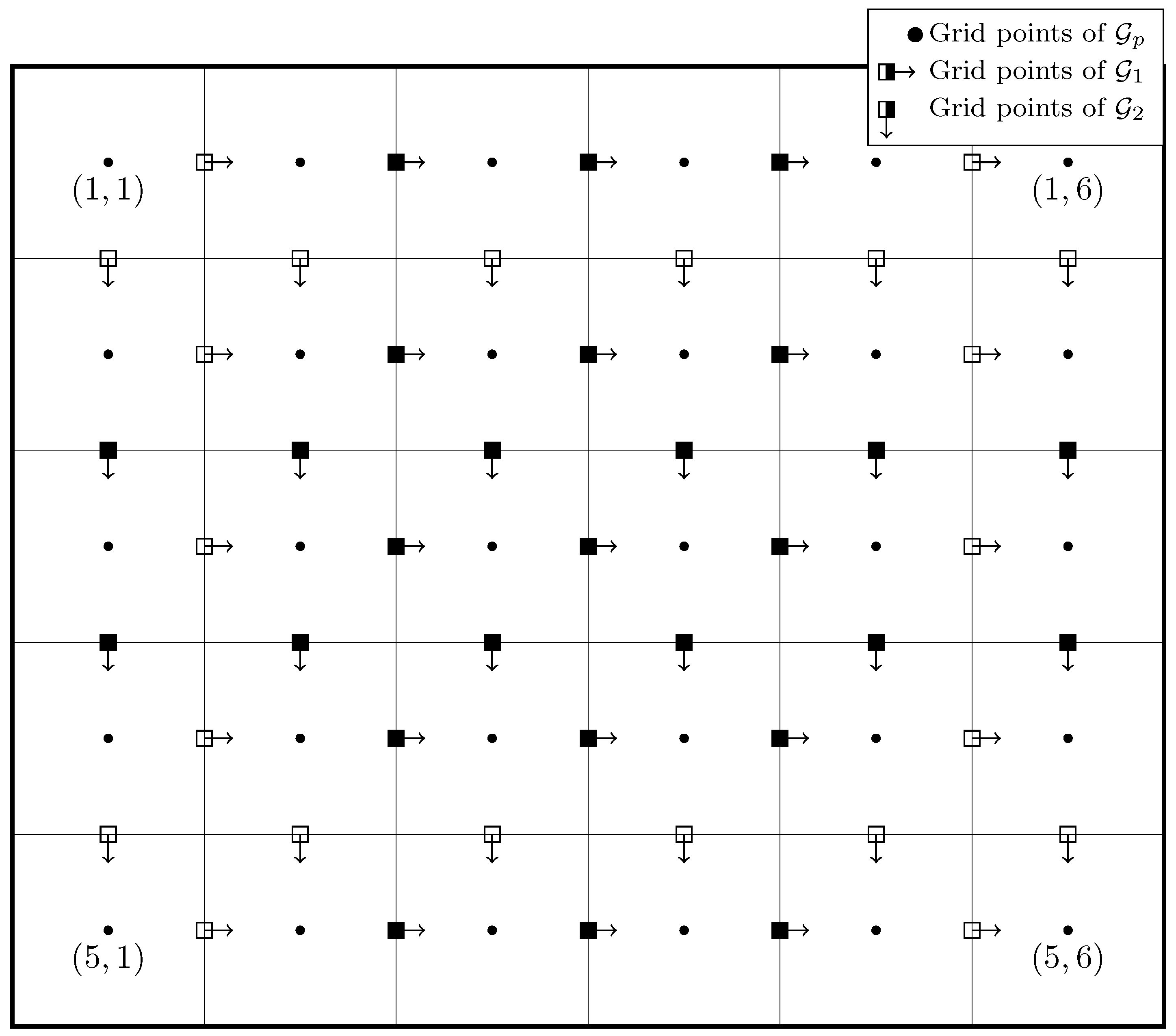
For the spatial discrete setting we assume that are given. Further, we consider with and . In contrast to [34] we assume no flow over the image boundary and set
See Figure 2 for an illustration. We approximate for by
and for and by
and similarly for the derivatives with respect to . Then we obtain
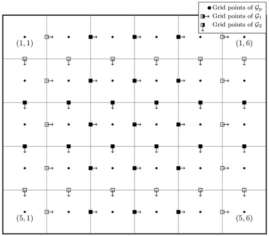
Figure 2.
Illustration of the grids, where empty boxes mean zero movement.
To discretize the data term in (7) we need to approximate . Since v is not defined on we use instead of v its averaged version given by
and similarly for in y-direction. Let the continuous function on be constructed from given values of T on by interpolation. Here we restrict our attention to bilinear interpolations, see (A3), but more sophisticated approaches are possible. In summary, the discrete registration problem reads
where is given by (8). We solve this nonlinear least squares problem by a Gauss-Newton like method described in the Appendix B.
Multilevel Strategy
As usual in optical flow and image registration we apply a coarse-to-fine strategy. First we iteratively smooth and downsample our given images. On the coarsest level we perform a registration to obtain a deformation on the coarse grid. We apply a bilinear interpolation v of this deformation to construct intermediate images on the finer level by
where are the start and end images at the new level. Then we use the alternating algorithm on this level with images to obtain deformations and intermediate images on this level. Going to the finer level by bilinear interpolation, we construct more intermediate images by interpolating between neighboring images with (9). We repeat this process until we reach the maximal number K of images and finest level. The multilevel strategy of the algorithm is sketched in Algorithm 1.
| Algorithm 1 Morphing Algorithm (informal). | |
| 1: | |
| 2: | create image stack on by smoothing and downsampling |
| 3: | solve (3) for with , for |
| 4: | |
| 5: | use bilinear interpolation to get v on from |
| 6: | obtain images from by (9) |
| 7: | while do |
| 8: | find image path and deformation path minimizing (3) with initialization |
| 9: | |
| 10: | if l > 0 then |
| 11: | use bilinear interpolation to get and on |
| 12: | for do |
| 13: | calculate intermediate images between with using (9) |
| 14: | |
3. Face Colorization
In this section, we describe a method to colorize a gray-scale image based on the morphing map between the luminance channel of a source image (template) and the present image (target). The idea consists in transferring of the chrominance channels from the source image to the target one. To this end, we work in the YUV color space. For the importance of the chrominance channels in color imaging, see, e.g., [41,42]. While in RGB images the color channels are highly correlated, the YUV space shows a suitable decorrelation between the luminance channel Y and the two chrominance channels . The transfer from the RGB space to YUV space is given by (see, e.g., [5])
Most of the colorization approaches are based on the hypothesis that the target image is the luminance channel of the desired image. Thus, the image colorization process is based on the computation of the unknown chrominance channels.
3.1. Luminance Normalization
The first step of the algorithm consists in transforming the RGB source image to the image by (10). The range of the target gray-value image and the Y channel of the source image may differ making the meaningful comparison between these images not possible.
To tackle this issue, most of state-of-the art methods use a technique called luminance remapping which was introduced in [43]. This affine mapping between images which aims to fit the average and the standard deviation of the target and the template images is defined as
where mean is the average of the pixel values, and var is the empirical variance.
3.2. Chrominance Transfer by the Morphing Maps
Next we compute the morphing map between the two gray-scale images and with model (3). This results in the deformation sequence which produces the resulting map from the template image to the target one by concatenation
Due to the discretization of the images, the map is defined, for images of size , on the discrete grid :
where is the position in the source image which corresponds to the pixel in the target image. Now we colorize the target image by computing its chrominance channels, denoted by at position x as
The chrominance channels of the target image are defined on the image grid , but usually . Therefore the values of the chrominance channels at have to be computed by interpolation. In our algorithm we use just bilinear interpolation which is defined for with , by
Finally, we compute a colorized RGB image from its luminance and the chrominance channels (11) by the inverse of (10):
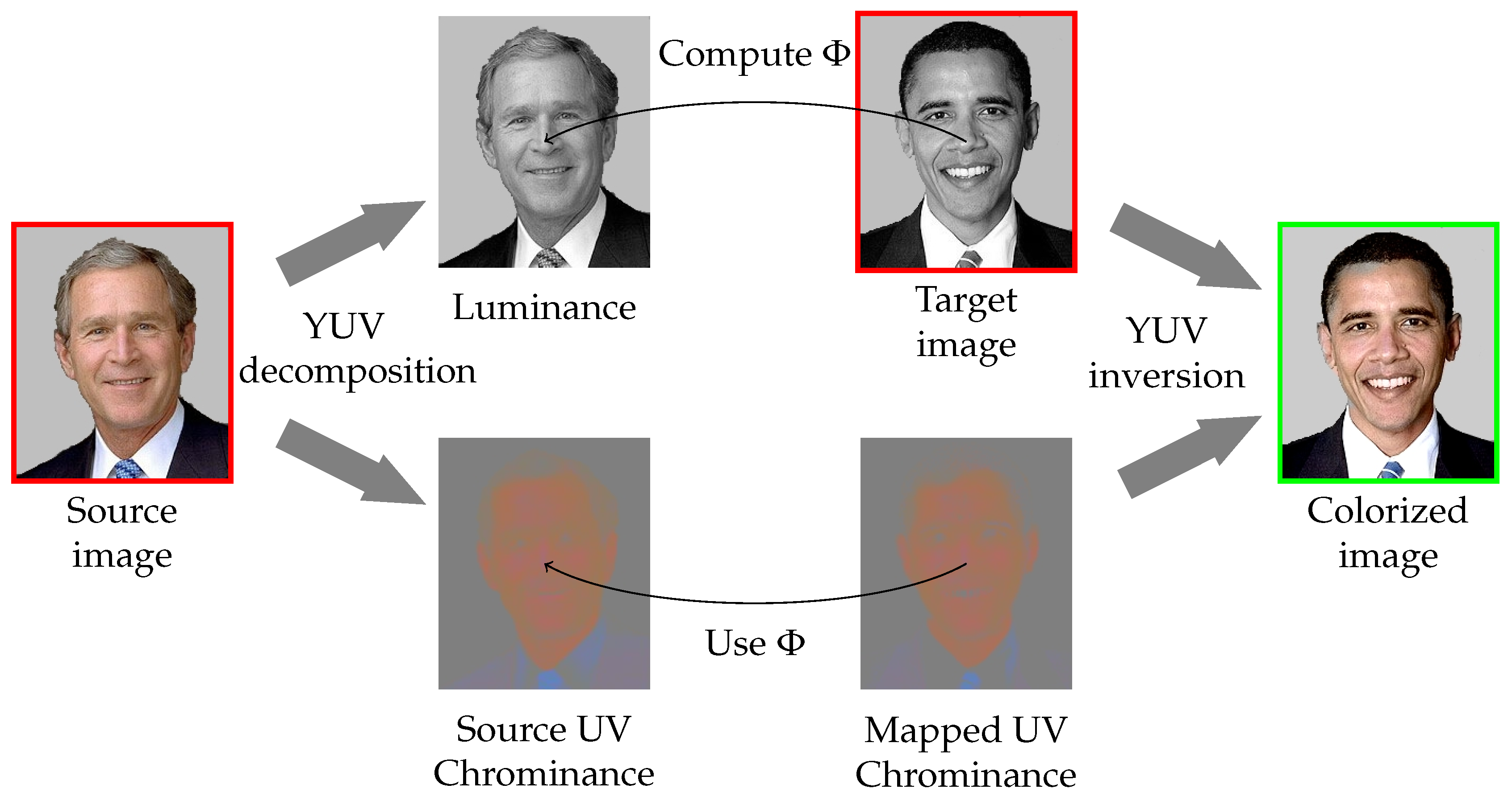
for all . Figure 3 (Image segements with unified background of George W. Bush https://commons.wikimedia.org/wiki/File:George-W-Bush.jpeg and Barack Obama https://commons.wikimedia.org/wiki/File:Barack_Obama.jpg both in public domain.) summarizes our color transfer method.
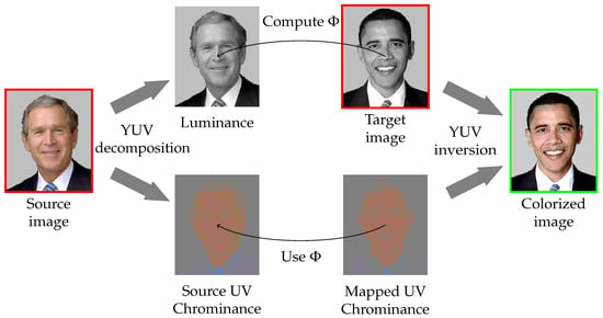
Figure 3.
Overview of the color transfer. The mapping is computed from Model (3) between the luminance channel of the source image and the target one. From this map, the chrominances of the source image are mapped. Finally, from these chrominances and the target image the colorization result is computed.
4. Variational Methods for Chrominance Postprocessing
Sometimes the color transfer computed from the morphing map can be disturbed by artifacts. To improve the results, post-processing steps are usually applied in the literature.
Variational approaches are frequently applied in image colorization either directly or as a post-processing step, see, e.g., [1,3,44]. For instance, the technique of Gupta et al. [6] uses the chrominance diffusion approach of Levin et al. [1].
In this paper, we propose a variational method with a total variation based regularization as a post-processing step to remove possible artifacts. We build up on the model [3] suggested by one of the authors. This variational model uses a functional with a specific regularization term to avoid ”halo effects”. More precisely, we consider the minimizer of
with
The first term in (13) is a coupled total variation term which enforces the chrominance channels to have a contour at the same location as the target gray-value image. The data fidelity term is the classical squared -norm of the differences of the given and the desired chrominance channels. Note that the model in [3] contains an additional box constraint.
The parameter manages the coupling of the chrominance channels with the luminance one. It has been shown in [3] that a parameter value around 25 can be used for most images. The parameter is related to the object size in the images. If some colors on large objects leak on small ones, this parameter has to be increased. On the other hand, if some artifacts are still present in the result, the value of has to be decreased. We apply the primal-dual Algorithm 2 to find the minimizer of the strictly convex model (13). It uses an update on the step time parameters and , as proposed by Chambolle and Pock [45], as well as a relaxation parameter to speed-up the convergence. Here we use the abbreviation and . Further, p is the dual variable which is pixel-wise in . The parameters and are intern time step sizes. The operator div stands for the discrete divergence and ∇ for the discrete gradient. Further, the proximal mapping is given pixel-wise, for by
| Algorithm 2 Minimization of (13). | |
| 1: | , |
| 2: | |
| 3: | , |
| 4: | for do |
| 5: | |
| 6: | |
| 7: | |
| 8: | |
| 9: | |
| 10: | |
As mentioned in the work of Deledalle et al. [38], the minimization of the TV- model produces a biased result. This bias causes a lost of contrast in the case of gray-scale images, whereas it is visible as a lost of colorfulness in the case of model (13). The authors of [38] describe an algorithm to remove such bias. In this paper, we propose to modify this method for our model (13) in order to enhance the result of Algorithm 2.
The CLEAR method of [38] relies on the refitting estimator of the data y from the biased estimation :
where is defined as the set of maps satisfying, :
where is the Jacobian of the biased estimator with respect to the data y:
contains some structural information of the biased estimator such as the jumps. A closed formula for can be given:
where . With Equation (15), the refitting process is as closer as possible to the original data.
The final algorithm is summarized in Algorithm 3. Note that it uses the result of Algorithm 1 as an input. The proximal mapping within the algorithm is defined pixel-wise, for variables and , as
where and are defined as in (14).
| Algorithm 3 Debiasing of Algorithm 2. | |
| 1: | , |
| 2: | |
| 3: | , |
| 4: | , |
| 5: | , |
| 6: | for do |
| 7: | |
| 8: | |
| 9: | |
| 10: | |
| 11: | |
| 12: | |
| 13: | |
| 14: | |
| 15: | |
| 16: | |
The results obtained at the different steps of the work-flow are presented for a particular image in Figure 4. First we demonstrate in Figure 4c that simply transforming the channels via the morphing map gives no meaningful results. Letting our morphing map act to the chrominance channels of our source image and applying (12) with the luminance of our target image we get , e.g., Figure 4d which is already a good result. However, the forehead of Obama contains an artifact; a gray unsuitable color is visible here. After a post-processing of the chrominance channels by our variational method the artifacts disappear as can be seen in Figure 4e.

Figure 4.
Illustration of the colorization steps of our algorithm. (a) The color source image; (b) The gray value target image; (c) The transport of the channel via the morphing map is not suited for colorization; (d) The result with our morphing method is already very good; (e) It can be further improved by our variational post-processing.
5. Numerical Examples
In this section, we compare our method with
- -
- the patch-based algorithm of Welsh et al. [8],
- -
- the patch-based method of Pierre et al. [3], and
- -
- the segmentation approach of Gupta et al. [6].
We implemented our morphing algorithm in Matlab 2016b and used the Matlab intern function for the bilinear interpolation. The parameters are summarized in Table 1. Here and K are the parameters for the morphing step. The parameters and appear in the variational model for post-processing and were only applied in three images. The number of deformations K depends on the size and details of the image, i.e., large detailed images need a larger K as small image having not so much details. Usually was a good choice for our experiments. The parameter controls the smoothness of the deformation, i.e., a small value leads to large movements which might not be reasonable, while for large values the deformations become zero and the image metamorphosis is just a blending. In our experiments, a value of magnitude lead to good results.

Table 1.
Parameters for our numerical experiments.
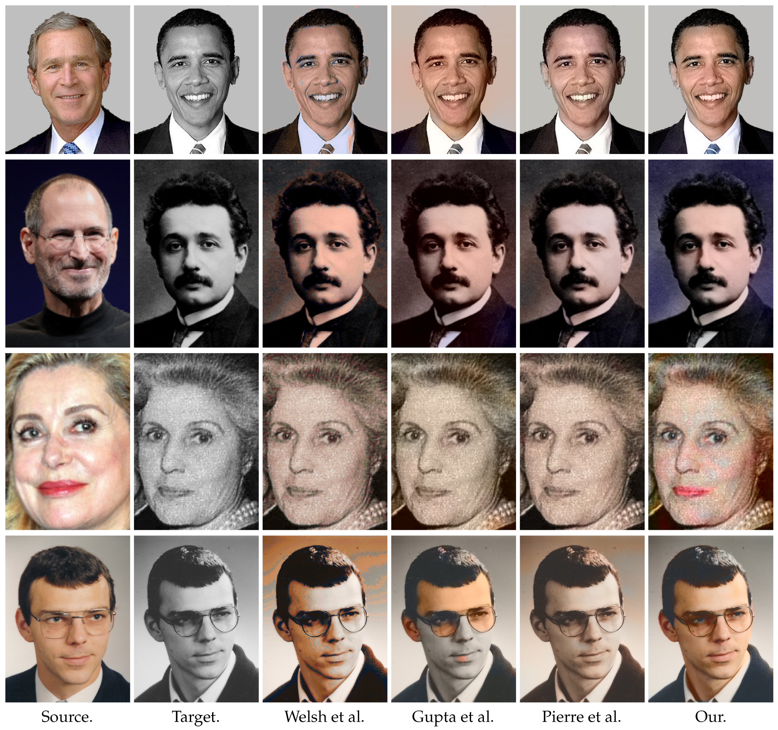
First we compare portraits in Figure 5 (Image segments of Steve Jobs https://commons.wikimedia.org/wiki/File:Steve_Jobs_Headshot_2010-CROP.jpg image courtesy of Matthew Yohe, Albert Einstein https://commons.wikimedia.org/wiki/File:Einstein_Portr_05936.jpg in public domain, Catherine Deneuve https://commons.wikimedia.org/wiki/File:Catherine_Deneuve_2010.jpg image courtesy of Georges Biard and Renée Deneuve https://commons.wikimedia.org/wiki/File:Ren%C3%A9e_Deneuve.jpg in public domain.) starting with the modern photographies in the first row. The approach of Welsh et al. [8] is based on a patch matching between images. The patch comparison is done with basic texture descriptors (intensity of the central pixel and standard-deviation of the patches). Since the background, as well as the skin are smooth, the distinction between them is unreliable if their intensities are similar. Moreover, since no regularization is used after the color transfer, some artifacts occur. For instance, some blue points appear on Obama’s face, see Figure 5, first row. The approach of Pierre et al. [3] is based on more sophisticated texture features for patches and applies a variational model with total variation like regularization. With this approach the artifacts mentioned above are less visible. Nevertheless, the forehead of Obama is purple which is unreliable. The method of Gupta et al. [6] uses texture descriptors after an over-segmentation, see, e.g., SLIC [10]. The texture descriptors are based on SURF and Gabor features. In the case of the Obama image, the descriptors are not able to distinguish the skin and other smooth parts, leading to a background color different from the source image. Our method is able to colorize the second image in a more reasonable way, i.e., face and background color are different and the tie gets a blue color. However, our methods is not perfect so far. For example part of the forehead of Obama becomes gray is due to the gray hair of Bush, which has a gray value closer to the forehead as to the hair of Obama.
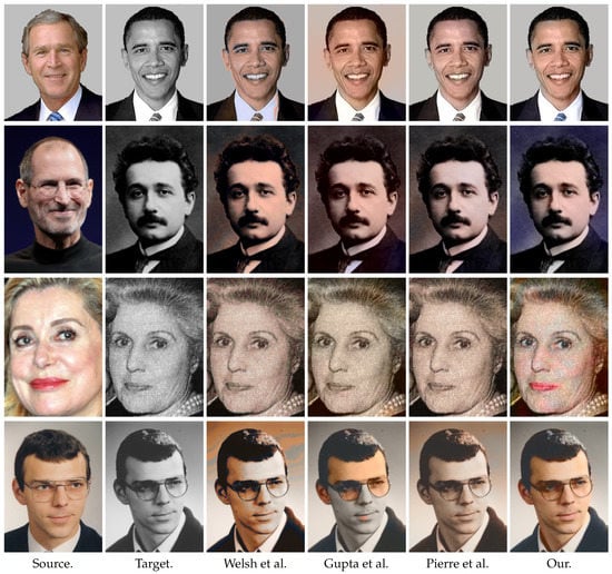
Figure 5.
Comparison of our approach with state-of-the-art methods on photographies. In contrast to these methods our model is not based on texture comparisons, but on the morphing of the shapes. Therefore it is able to handle faces images, where the background has frequently a similar texture as the skin.
The second and the third rows of Figure 5 focus on the colorization of old photographies. This challenging problem is a real application of image colorization which is sought, e.g., by the cinema industry. Note that the texture of old images are disturbed by the natural grain which is not the case in modern photography. Thus, the texture comparison is unreliable for this application. This issue is visible in all the comparison methods. For the portrait of Einstein the background is not colorized with the color of the source. Moreover, the color of the skin is different from those of the person in the source image. For the picture of Deneuve, the color of her lips is not transferred to the target image (Deneuve’s mother) with the state-of-the-art texture-based algorithms. With our morphing approach, the shapes of the faces are mapped. Thus, the lips, as well as the eyes and the skin are well colorized with a color similar to the source image. In the last row we have two images of the same person. Here the state-of-the-art-texture-based methods give unlikely results, especially the methods of Welsh et al. and Gupta et al. lead to a non smooth colorization of the background and the face, respectively. Our method provides a reasonable result with only small artifacts around the glasses.
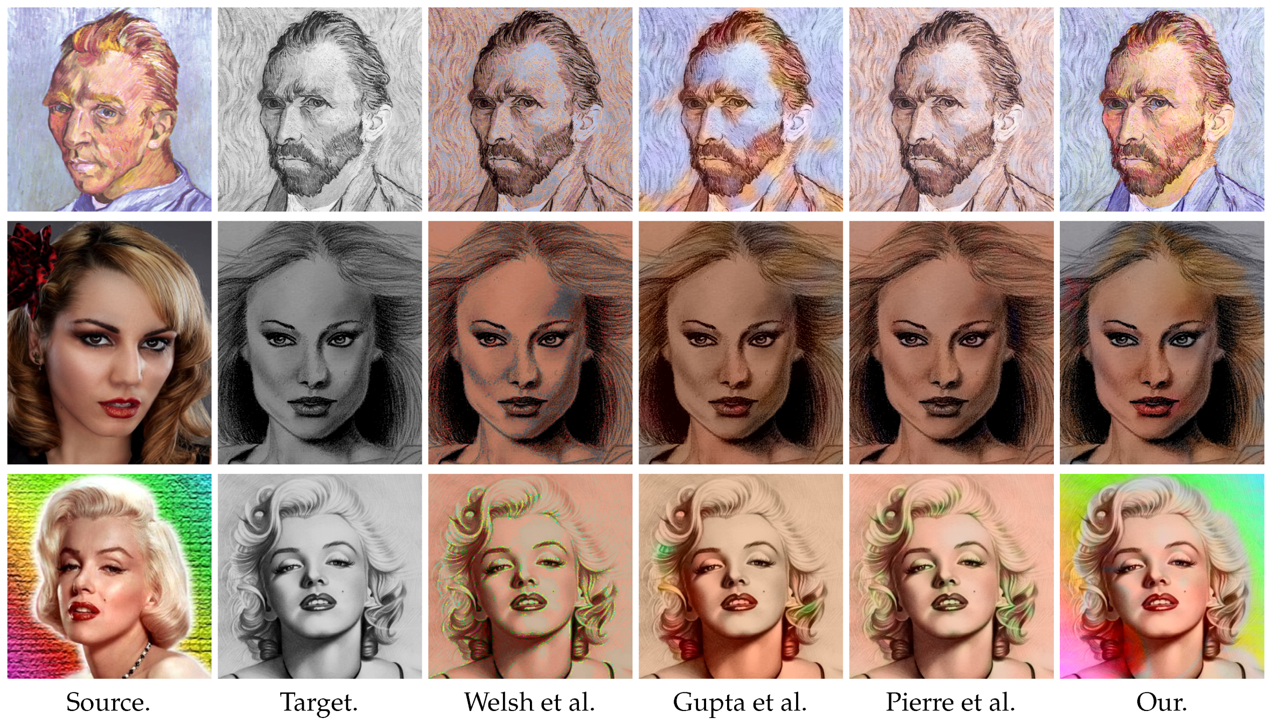
In Figure 6 (Image segments of self-portraits of Vincent van Gogh https://commons.wikimedia.org/wiki/File:Vincent_Willem_van_Gogh_102.jpg and https://commons.wikimedia.org/wiki/File:Vincent_van_Gogh_-_Self-Portrait_-_Google_Art_Project.jpg both in public domain, a photography of a woman https://pixabay.com/en/woman-portrait-face-model-canon-659352/ licensed CC0, a drawing of a woman https://pixabay.com/en/black-and-white-drawing-woman-actor-1724363/ licensed CC0, a color image of Marilyn Monroe https://www.flickr.com/photos/7477245@N05/5272564106 created by Luiz Fernando Reis, and a drawing of Marilyn Monroe https://pixabay.com/en/marilyn-monroe-art-draw-marilyn-885229/ licensed CC0), we provide results including painted images. Note that we use the same Van Gogh self-portraits as in [31]. Due to the low contrast of the ear and suit to the background we add here the same segmentation information as in [31], which means our images are two dimensional during the calculation for the results shown in the first row of Figure 6. In these examples the similarity of the shapes between the source and target images is again more reliable than the matching of the textures so that only our morphing approach produces suitable results. Consider in particular the lips of the woman in the second and third row. A non post-processed result for the woman in the second row is shown in Figure 7. Comparing the two images we see that only small details change but most of the colorization is done by the morphing.
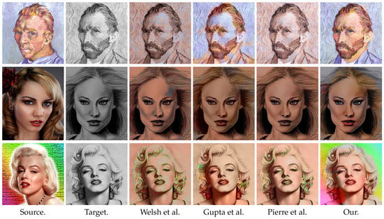
Figure 6.
Results including painted faces. Only our morphing method is able to colorize the target images in an authentic way.
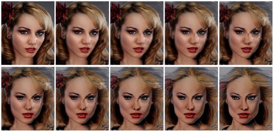
Figure 7.
Color transport along the image path.
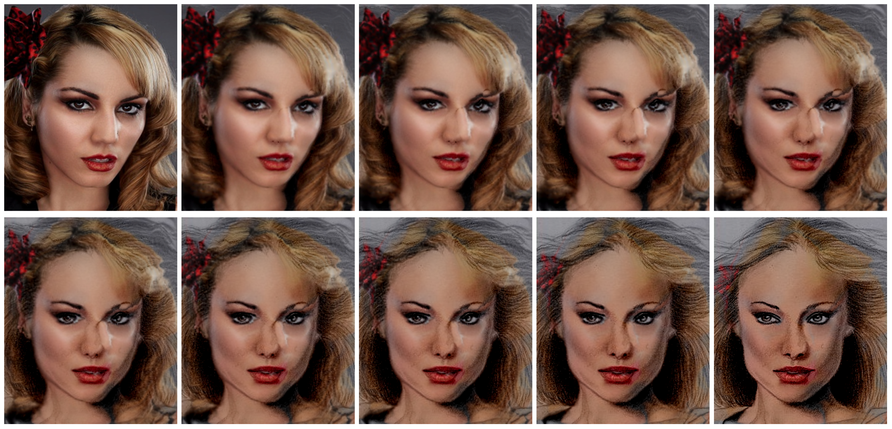
Figure 7 visualizes the path of the color transfer. As the morphing approach calculates at the same time an image and mapping path, we can not only show the final colorization result, but also the way the color is transported along this path. We illustrate this by the image in second row of Figure 6. The UV channels are transported via the mapping path of the Y channels of the source and the target images, where every second image along the path is shown. We see that even though the right part of the images undergoes large transformations, the eyes and the mouth are moved to the correct places. Note that the final image does not contain a post-processing, in contrast to those in the second row of Figure 6. However, the result is already quite good.
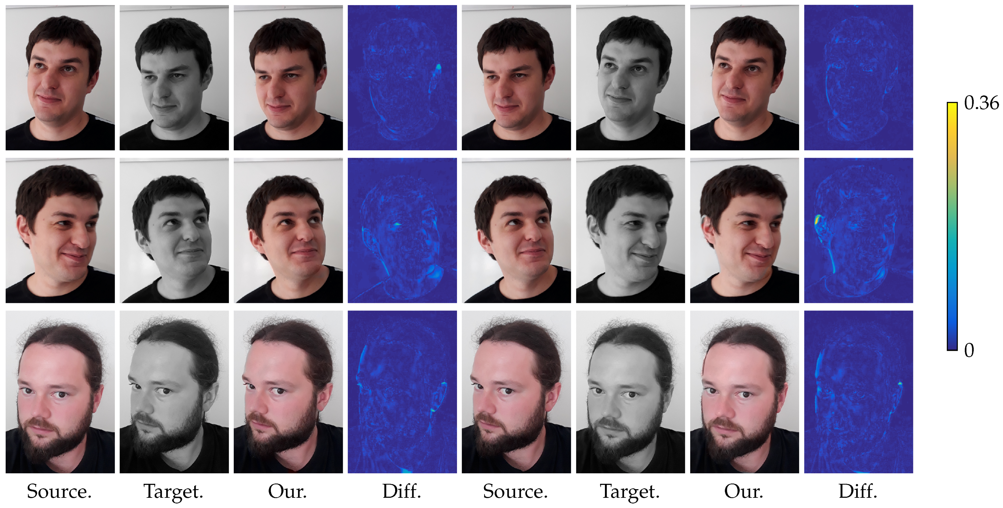
Figure 8 is included to evaluate the quality of our colorization method. We took two photographs of the same person in different poses. Assuming that the color of the person does not change due to the movement, we have a ground truth target image and can do a quantitative comparison using the PSNR. We see that the visual superiority of our result is confirmed by the much higher PSNR.

Figure 8.
Results on a color image turned into a gray-scale one for a quantitative comparison. The qualitative comparisons with the state-of-the-art methods are confirmed by the PSNR measures.
In Figure 9 we considered three RGB image pairs. Using the luminance of one of the images as target and the other one as source and conversely we colorized the target image and computed the PSNR. In Table 2 the PSNR values of the colorization with our method and the state-of-the-art methods are shown. The performance of our method is very convincing for all these example images.

Figure 9.
Multiple colorizations of known RGB-images with difference plots measured in Euclidean distance in .

Table 2.
Comparison of the different PSNR values for the image pairs in Figure 9.
Remark (Limitations of our approach).
In all our experiments our method leads to good results and outperforms the state-of-the-art colorization methods. However, the method is not perfect and the face images can not be arbitrarily deformed. Since the morphing is only done in the Y channel, the illumination of the faces should be similar. For example there is a shadow on the left side of the images in the second row of Figure 5. Mirroring one of the images would lead to bad matching results. The same holds true for the features themselves, so we can not expect to match bright hair perfectly to dark hair, as we see for example in Figure 4d.
Since the deformations are close to diffeomorphisms, features should not be excluded or appear. For example, the left eye in the last row of Figure 9 starts in the middle of the face and moves to the edge, so a part of the skin-color stays in the eye. Similarly in the second matching here the eye moves from the edge to the inside, so the skin obtains the color from the background.
By a proper initialization the faces should be aligned in such a way that there are no similar features atop of each other, e.g., a left eye in the source should not be atop of the right eye of the target. However with more prior knowledge we could use the given features as landmarks and perform a landmark matching, e.g., [46], for the initialization on the coarsest level.
6. Conclusions
In this paper, we propose an finite difference method to compute a morphing map between a source and a target gray-value image. This map enables us to transfer the color from the source image to the target one, based on the shapes of the faces. An additional variational post-processing step with a luminance guided total variation regularization and an update to make the result unbiased may be added to remove some possible artifacts. The results are very convincing and outperform state-of-the-art approaches on historical photographies.
Let us notice some special issues of our approach in view of an integration into a more global framework for an exemplar-based image and video colorization. First of all, our method works well on faces and on object with similar shapes, but when this hypothesis is not fulfilled, some artifacts can appear. Therefore, instead of using our algorithm on full images, a face detection algorithm can be used to focus on the face colorization. Let us remark that faces in image can be detected by efficient, recent methods, see, e.g., [47]. In future work, the method will be integrated into a complete framework for exemplar-based image and video colorization.
Second, the morphing map has to be computed between images with the same size. This issue can be easily solved with a simple interpolation of the images. Keeping the ratio between the width and the height of faces similar, the distortion produced by such interpolation is small enough to support our method.
Acknowledgments
Funding by the German Research Foundation (DFG) within the project STE 571/13-1 is gratefully acknowledged.
Author Contributions
All the three authors have substantially contributed to the paper. The paper is the outcome of many joint and fruitful discussions J. Persch and G. Steidl had with F. Pierre during the months the later was a Postdoc at the University at Kaiserslautern (Germany). Therefore it is not possible to split the contributions. However, J. Persch was the leading expert concerning morphing and F. Pierre concerning color image processing.
Conflicts of Interest
The authors declare no conflict of interest.
Appendix A. Solution of the Image Sequence Problem
Fixing , resp., leads to the image sequence problem (6). In the following we show how this problem can be solved via the linear system of equations arising from Euler-Lagrange equation of the functional. We mainly follow [31].
The terms in containing are
Assuming that is a diffeomorphism, the variable transform gives
Setting
the Euler-Lagrange equations read for as
We introduce
which can be computed for each since the , are given. Then (A1) can be rewritten for as
In matrix-vector form, this reads with
for fixed and as
Assuming that which is the case in practical applications, the matrix A is irreducible diagonal dominant and thus invertible.
Appendix B. Gauss-Newton Method for the Registation Problem
We consider the nonlinear least squares problem in (7)
Let us first write in a convenient matrix-vector notation. Using , and
and similarly and we obtain
where denotes the Frobenius norm of matrices. Reshaping the , columnwise into a vectors and (where we keep the notation) and using tensor products ⊗ of matrices
the regularizing term can be rewritten as
The nonlinear data term in the registration problem with the columnwise reshaped image of and of reads
We linearize the term at a previous iterate , i.e.,
We comment on the computation of below. Then we consider
The gradient is given by
Setting the gradient to zero we obtain for
As we want to minimize , the next iterate is given by
where is the smallest number such that , if is not zero.
Finally we comment on the computation of
Since is computed by linear interpolation from , Then we have for an arbitrary point , that
Then
Hence the derivatives can be calculated from the forward differences of T in x- resp. y-direction and appropriate weighting.
References
- Levin, A.; Lischinski, D.; Weiss, Y. Colorization using optimization. ACM Trans. Graph. 2004, 23, 689–694. [Google Scholar] [CrossRef]
- Irony, R.; Cohen-Or, D.; Lischinski, D. Colorization by example. In Proceedings of the 16th Eurographics Conference on Rendering Techniques, Konstanz, Germany, 29 June 29–1 July 2005; pp. 201–210. [Google Scholar]
- Pierre, F.; Aujol, J.F.; Bugeau, A.; Papadakis, N.; Ta, V.T. Luminance-chrominance model for image colorization. SIAM J. Imaging Sci. 2015, 8, 536–563. [Google Scholar] [CrossRef]
- Yatziv, L.; Sapiro, G. Fast image and video colorization using chrominance blending. IEEE Trans. Image Process. 2006, 15, 1120–1129. [Google Scholar] [CrossRef] [PubMed]
- Jack, K. Video Demystified: A Handbook for the Digital Engineer; Elsevier: Amsterdam, The Netherlands, 2011. [Google Scholar]
- Gupta, R.K.; Chia, A.Y.S.; Rajan, D.; Ng, E.S.; Zhiyong, H. Image colorization using similar images. In Proceedings of the 20th ACM International Conference on Multimedia, Nara, Japan, 29 October–2 November 2012; pp. 369–378. [Google Scholar]
- Horiuchi, T. Colorization algorithm using probabilistic relaxation. Image Vis. Comput. 2004, 22, 197–202. [Google Scholar] [CrossRef]
- Welsh, T.; Ashikhmin, M.; Mueller, K. Transferring color to greyscale images. ACM Trans. Graph. 2002, 21, 277–280. [Google Scholar] [CrossRef]
- Efros, A.A.; Leung, T.K. Texture synthesis by non-parametric sampling. In Proceedings of the 7th IEEE International Conference on Computer Vision, Kerkyra, Greece, 20–27 September 1999; Volume 2, pp. 1033–1038. [Google Scholar]
- Achanta, R.; Shaji, A.; Smith, K.; Lucchi, A.; Fua, P.; Süsstrunk, S. SLIC superpixels compared to state-of-the-art superpixel methods. IEEE Trans. Pattern Anal. Mach. Intell. 2012, 34, 2274–2282. [Google Scholar] [CrossRef] [PubMed]
- Chen, T.; Wang, Y.; Schillings, V.; Meinel, C. Grayscale image matting and colorization. In Proceedings of the Asian Conference on Computer Vision, Jeju Island, Korea, 27–30 January 2004; pp. 1164–1169. [Google Scholar]
- Charpiat, G.; Hofmann, M.; Schölkopf, B. Automatic image colorization via multimodal predictions. In European Conference on Computer Vision; Springer: Berlin/Heidelberg, Germany, 2008; pp. 126–139. [Google Scholar]
- Chia, A.Y.S.; Zhuo, S.; Kumar, R.G.; Tai, Y.W.; Cho, S.Y.; Tan, P.; Lin, S. Semantic colorization with internet images. ACM Trans. Graph. 2011, 30, 156. [Google Scholar] [CrossRef]
- Zhang, R.; Isola, P.; Efros, A.A. Colorful image colorization. In European Conference on Computer Vision; Springer: Berlin/Heidelberg, Germany, 2016; pp. 1–16. [Google Scholar]
- Smythe, D.B. A Two-Pass Mesh Warping Algorithm for Object Transformation and Image Interpolation; Technical report; ILM Technical Memo Department, Lucasfilm Ltd.: San Francisco, CA, USA, 1990. [Google Scholar]
- Wolberg, G. Digital Image Warping; IEEE Computer Society Press: Los Alamitos, CA, USA, 1990; Volume 10662. [Google Scholar]
- Wolberg, G. Image morphing: A survey. Vis. Comput. 1998, 14, 360–372. [Google Scholar] [CrossRef]
- Miller, M.I.; Younes, L. Group actions, homeomorphisms, and matching: A general framework. Int. J. Comput. Vis. 2001, 41, 61–84. [Google Scholar] [CrossRef]
- Trouvé, A.; Younes, L. Local geometry of deformable templates. SIAM J. Math. Anal. 2005, 37, 17–59. [Google Scholar] [CrossRef]
- Trouvé, A.; Younes, L. Metamorphoses through Lie group action. Found. Comput. Math. 2005, 5, 173–198. [Google Scholar] [CrossRef]
- Christensen, G.E.; Rabbitt, R.D.; Miller, M.I. Deformable templates using large deformation kinematics. IEEE Trans. Image Process. 1996, 5, 1435–1447. [Google Scholar] [CrossRef] [PubMed]
- Dupuis, P.; Grenander, U.; Miller, M.I. Variational problems on flows of diffeomorphisms for image matching. Q. Appl. Math. 1998, 56, 587–600. [Google Scholar] [CrossRef]
- Trouvé, A. An infinite dimensional group approach for physics based models in pattern recognition. Int. J. Comput. Vis. 1995, 28, 213–221. [Google Scholar] [CrossRef]
- Trouvé, A. Diffeomorphisms groups and pattern matching in image analysis. Int. J. Comput. Vis. 1998, 28, 213–221. [Google Scholar] [CrossRef]
- Beg, M.F.; Miller, M.I.; Trouvé, A.; Younes, L. Computing large deformation metric mappings via geodesic flows of diffeomorphisms. Int. J. Comput. Vis. 2005, 61, 139–157. [Google Scholar] [CrossRef]
- Richardson, C.L.; Younes, L. Metamorphosis of images in reproducing kernel Hilbert spaces. Adv. Comput. Math. 2016, 42, 573–603. [Google Scholar] [CrossRef]
- Hong, Y.; Joshi, S.; Sanchez, M.; Styner, M.; Niethammer, M. Metamorphic geodesic regression. Med. Image Comput. Comput. Assist. Interv. 2012, 15, 197–205. [Google Scholar] [PubMed]
- Younes, L. Shapes and Diffeomorphisms; Springer: Berlin, Germany, 2010. [Google Scholar]
- Miller, M.I.; Trouvé, A.; Younes, L. Hamiltonian systems and optimal control in computational anatomy: 100 years since D’Arcy Thompson. Annu. Rev. Biomed. Eng. 2015, 17, 447–509. [Google Scholar] [CrossRef] [PubMed]
- Miller, M.I.; Trouvé, A.; Younes, L. On the metrics and Euler-Lagrange equations of computational anatomy. Annu. Rev. Biomed. Eng. 2002, 4, 375–405. [Google Scholar] [CrossRef] [PubMed]
- Berkels, B.; Effland, A.; Rumpf, M. Time discrete geodesic paths in the space of images. SIAM J. Imaging Sci. 2015, 8, 1457–1488. [Google Scholar] [CrossRef]
- Christensen, G.E.; Johnson, H.J. Consistent image registration. IEEE Trans. Med. Imaging 2001, 20, 568–582. [Google Scholar] [CrossRef] [PubMed]
- Fischer, B.; Modersitzki, J. Curvature based image registration. J. Math. Imaging Vis. 2003, 18, 81–85. [Google Scholar] [CrossRef]
- Haber, E.; Modersitzki, J. A multilevel method for image registration. SIAM J. Sci. Comput. 2006, 27, 1594–1607. [Google Scholar] [CrossRef]
- Han, J.; Berkels, B.; Droske, M.; Hornegger, J.; Rumpf, M.; Schaller, C.; Scorzin, J.; Urbach, H. Mumford–Shah Model for one-to-one edge matching. IEEE Trans. Image Process. 2007, 16, 2720–2732. [Google Scholar] [CrossRef] [PubMed]
- Modersitzki, J. Numerical Methods for Image Registration; Oxford University Press: Oxford, UK, 2004. [Google Scholar]
- Modersitzki, J. FAIR: Flexible Algorithms for Image Registration; SIAM: Philadelphia, PA, USA, 2009. [Google Scholar]
- Deledalle, C.A.; Papadakis, N.; Salmon, J.; Vaiter, S. CLEAR: Covariant LEAst-square Refitting with applications to image restoration. SIAM J. Imaging Sci. 2017, 10, 243–284. [Google Scholar] [CrossRef]
- Miller, M.I.; Christensen, G.E.; Amit, Y.; Grenander, U. Mathematical textbook of deformable neuroanatomies. Proc. Natl. Acad. Sci. USA 1993, 90, 11944–11948. [Google Scholar] [CrossRef] [PubMed]
- Yuan, J.; Schnörr, C.; Steidl, G. Simultaneous higher order optical flow estimation and decomposition. SIAM J. Sci. Comput. 2007, 29, 2283–2304. [Google Scholar] [CrossRef]
- Bertalmio, M. Image Processing for Cinema; CRC Press: Boca Raton, FL, USA, 2014. [Google Scholar]
- Nikolova, M.; Steidl, G. Fast Hue and Range Preserving Histogram Specification: Theory and New Algorithms for Color Image Enhancement. IEEE Trans. Image Process. 2014, 23, 4087–4100. [Google Scholar] [CrossRef] [PubMed]
- Hertzmann, A.; Jacobs, C.E.; Oliver, N.; Curless, B.; Salesin, D.H. Image analogies. In Proceedings of the 28th Annual Conference on Computer Graphics and Interactive Techniques, Los Angeles, CA, USA, 12–17 August 2001; pp. 327–340. [Google Scholar]
- Peter, P.; Kaufhold, L.; Weickert, J. Turning diffusion-based image colorization into efficient color compression. IEEE Trans. Image Process. 2016, 26, 860–869. [Google Scholar] [CrossRef] [PubMed]
- Chambolle, A.; Pock, T. A first-order primal-dual algorithm for convex problems with applications to imaging. J. Math. Imaging Vis. 2011, 40, 120–145. [Google Scholar] [CrossRef]
- Joshi, S.C.; Miller, M.I. Landmark matching via large deformation diffeomorphisms. IEEE Trans. Image Process. 2000, 9, 1357–1370. [Google Scholar] [CrossRef] [PubMed]
- Chen, D.; Hua, G.; Wen, F.; Sun, J. Supervised transformer network for efficient face detection. In European Conference on Computer Vision; Springer: Cham, Switzerland, 2016; pp. 122–138. [Google Scholar]
© 2017 by the authors. Licensee MDPI, Basel, Switzerland. This article is an open access article distributed under the terms and conditions of the Creative Commons Attribution (CC BY) license (http://creativecommons.org/licenses/by/4.0/).


