Baseline Fusion for Image and Pattern Recognition—What Not to Do (and How to Do Better)

Abstract

The ever-increasing demand for a reliable inference capable of handling unpredictable challenges of practical application in the real world has made research on information fusion of major importance; indeed, this challenge is pervasive in a whole range of image understanding tasks. In the development of the most common type—score-level fusion algorithms—it is virtually universally desirable to have as a reference starting point a simple and universally sound baseline benchmark which newly developed approaches can be compared to. One of the most pervasively used methods is that of weighted linear fusion. It has cemented itself as the default off-the-shelf baseline owing to its simplicity of implementation, interpretability, and surprisingly competitive performance across a widest range of application domains and information source types. In this paper I argue that despite this track record, weighted linear fusion is not a good baseline on the grounds that there is an equally simple and interpretable alternative—namely quadratic mean-based fusion—which is theoretically more principled and which is more successful in practice. I argue the former from first principles and demonstrate the latter using a series of experiments on a diverse set of fusion problems: classification using synthetically generated data, computer vision-based object recognition, arrhythmia detection, and fatality prediction in motor vehicle accidents. On all of the aforementioned problems and in all instances, the proposed fusion approach exhibits superior performance over linear fusion, often increasing class separation by several orders of magnitude.

1. Introduction

Score-level fusion of information is pervasive in a wide variety of problems. From predictions of the price of French vintage wine using the fusion of predictions based on rainfall and temperature data [1], to sophisticated biometrics algorithms which fuse similarity measures based on visual, infrared face appearance, or gait characteristics [2,3,4,5], the premise of information fusion is the same: the use of multiple information sources facilitates the making of better decisions [6,7].

Whatever the specific problem, the effectiveness of a specific information fusion methodology needs to be demonstrated. If possible this should be done by comparing its performance against the current state-of-the-art. However this is often prohibitively difficult in practice. For example, in some cases the state-of-the-art may not be readily available for evaluation—the original code may not have been released and re-implementation may be overly time-consuming, the algorithm may not have been described in sufficient detail, the technology may be proprietary and costly to purchase, etc. In other cases there may not be a clear state-of-the-art because the particular problem at hand has not been addressed before. In such circumstances it is useful to compare the novel methodology with a simple yet sensible baseline [8].

Probably the simplest choices for the baseline would be the performances achieved using individual information sources which are being fused. However this is an excessively low bar for comparison. Instead what is widely done by authors across the research spectrum is to use simple weighted fusion of individual scores as a reference. In the present paper I analyse this choice, present theoretical arguments against it, and its lieu propose an alternative. The proposed alternative is inherently more principled than the aforementioned baseline, while being no more complex, either computationally or conceptually.

2. Uninformed Information Fusion

Let us start by formalizing the problem considered in this paper. I adopt the broad paradigm of so-called data source identification and matching. In particular, I assume that the available data comprises a set of n sensed observations, $\mathbf{X}=\left\{{\mathbf{x}}_i\right\}=\{{\mathbf{x}}_1,\dots ,{\mathbf{x}}_n\}$, which correspond to different modalities sensing the same data source. Furthermore, I assume that there are functions (i.e., algorithms) ${\varphi }_1,\dots ,{\varphi }_n$ which quantify how well a particular observation ${\mathbf{x}}_i$ matches a specific data source. Without loss of generality I assume $0\le {\varphi }_i\left({\mathbf{x}}_i\right)<\infty$, where 0 indicates the best possible match, and $\to \infty$ the worst i.e., ${\varphi }_i\left({\mathbf{x}}_i\right)$ can be thought of a quasi-distance—’quasi-’ to emphasise that it is not required that ${\varphi }_i\left({\mathbf{x}}_i\right)$ meets the strict conditions required of a metric. Note that the aforestated setting describes observations in the most general sense, e.g., these may be feature vectors (such as rasterized appearance images or SIFT descriptors in computer vision), sets of vectors, and so on, and they do not need to be of the same type (for example, some may be vectors, others sequences) or dimensionalities.

As noted in the previous section, we are looking for a simple way of fusing different matching decisions ${\varphi }_i\left({\mathbf{x}}_i\right)$ in a simple manner which is a reasonable baseline in an uninformed setting, that is, without exploiting any particular properties of different functions ${\varphi }_i$ or observations ${\mathbf{x}}_i$. A common one pervasively used in the literature is weighted linear fusion, which can be expressed as follows:

$$\mathsf{\Phi }({\mathbf{x}}_1,\dots ,{\mathbf{x}}_n;{\varphi }_1,\dots ,{\varphi }_n,w_1,\dots ,w_n)=\sum _{i=1}^n\left[w_i\times {\varphi }_i\left({\mathbf{x}}_i\right)\right],$$

(1)

where:

$$\forall i=1,\dots ,n.w_i\ge 0,\mathrm{and}\sum _{i=1}^n{w}_i=1.$$

(2)

Here $\mathsf{\Phi }({\mathbf{x}}_1,\dots ,{\mathbf{x}}_n;{\varphi }_1,\dots ,{\varphi }_n,w_1,\dots ,w_n)$ is the fused matching score which is derived by simply combining different ${\varphi }_i\left({\mathbf{x}}_i\right)$, and (2) ensures that the condition $0\le {\varphi }_i\left({\mathbf{x}}_i\right)<\infty$ is maintained for $\mathsf{\Phi }({\mathbf{x}}_1,\dots ,{\mathbf{x}}_n;{\varphi }_1,\dots ,{\varphi }_n,w_1,\dots ,w_n)$ as well, i.e., that it is the case that $0\le \mathsf{\Phi }({\mathbf{x}}_1,\dots ,{\mathbf{x}}_n;{\varphi }_1,\dots ,{\varphi }_n,w_1,\dots ,w_n)<\infty$.

The fusion approach described by (1) can also be rewritten more simply as:

$$\begin{array}{cc}\hfill \mathsf{\Phi }& ({\mathbf{x}}_1,\dots ,{\mathbf{x}}_n;{\varphi }_1,\dots ,{\varphi }_n,w_1,\dots ,w_n)=\hfill \end{array}$$

(3)

$$\widehat{\mathsf{\Phi }}({\mathbf{x}}_1,\dots ,{\mathbf{x}}_n;{\varphi }_1,\dots ,{\varphi }_n,w_1,\dots ,w_n)=\sum _{i=1}^n\left[\frac{1}{n}\times {\widehat{\varphi }}_i({\mathbf{x}}_i,w_i,n)\right],$$

(4)

where:

$${\widehat{\varphi }}_i({\mathbf{x}}_i,w_i,n)=n\times w_i\times {\varphi }_i\left({\mathbf{x}}_i\right).$$

(5)

Here the original weighted linear fusion of the contributing terms ${\varphi }_i\left({\mathbf{x}}_i\right)$ in (1) has been replaced by unweighted linear fusion of terms ${\widehat{\varphi }}_i({\mathbf{x}}_i,w_i,n)$ which adjust the magnitudes of the fused scores directly. This can be achieved simply by considering the statistics of the distributions of different ${\varphi }_i\left({\mathbf{x}}_i\right)$ and the corresponding prediction, and without any knowledge of what different features ${\mathbf{x}}_i$ represent or what form different ${\varphi }_i$ have, i.e., while maintaining the premise of uninformed fusion.

It can be readily seen that the described fusion approach fits the conditions specified in the proceeding section—namely, simplicity (both methodological and that of implementation) and broad applicability. Although simple, uninformed fusion demonstrates remarkably good performance across a wide span of different data types and domains, ranging from dementia screening [9] to multimodal biometric identification [2,10].

$${\mathsf{\Phi }}_o({\mathbf{x}}_1,\dots ,{\mathbf{x}}_n;{\varphi }_1,\dots ,{\varphi }_n,{\omega }_1,\dots ,{\omega }_n)=\sqrt{{\sum }_{i=1}^n\left[{\omega }_i\times {\varphi }_i{\left({\mathbf{x}}_i\right)}^2\right]},$$

(6)

where as before:

$$\forall i=1,\dots ,n.{\omega }_i\ge 0,\mathrm{and}\sum _{i=1}^n{\omega }_i=1.$$

(7)

$$\begin{array}{cc}\hfill {\mathsf{\Phi }}_o& ({\mathbf{x}}_1,\dots ,{\mathbf{x}}_n;{\varphi }_1,\dots ,{\varphi }_n,{\omega }_1,\dots ,{\omega }_n)=\hfill \end{array}$$

(8)

$$\begin{array}{c}{\widehat{\mathsf{\Phi }}}_o({\mathbf{x}}_1,\dots ,{\mathbf{x}}_n;{\varphi }_1,\dots ,{\varphi }_n,{\omega }_1,\dots ,{\omega }_n)=\sqrt{\sum _{i=1}^n\left[\frac{1}{n}\times {\tilde{\varphi }}_i{({\mathbf{x}}_i,{\omega }_i,n)}^2\right]},\hfill \end{array}$$

(9)

where, analogously to (5), the adjusted fusion scores can be expressed as:

$$\begin{array}{c}\hfill {\tilde{\varphi }}_i({\mathbf{x}}_i,{\omega }_i,n)=\sqrt{n}\times {\omega }_i\times {\varphi }_i\left({\mathbf{x}}_i\right).\end{array}$$

(10)

The formulation in (9) can be readily recognized as the quadratic mean, in engineering also commonly referred to as the root mean square (RMS), of the n terms ${\tilde{\varphi }}_i({\mathbf{x}}_i,{\omega }_i,n)$.

Before proceeding with a formal analysis of the two fusion approaches, it is insightful to gain an intuitive understanding of the difference between them. Note that simple linear fusion described in (4) treats different scores as effectively interchangeable—a decrease in one score is exactly compensated by an increase in another score by the same amount. This is sensible when the scores correspond to the same measurement which is merely repeated. The described fusion can then be seen as a way of reducing measurement error, assuming that measurement is unbiased and that errors are identically and independently distributed [11]. However this is a rather trivial case of fusion and in practice one is more commonly interested in fusion of different types of data modalities. Indeed, in practice it is often the explicit aim to try to use information sources which vary independently, and attempt to exploit best their complementary natures [12]. In such instances different scores are best treated as describing a source in orthogonal directions, thereby giving rise to a feature vector ${\left[{\tilde{\varphi }}_1\left({\mathbf{x}}_1\right),\dots ,{\tilde{\varphi }}_n\left({\mathbf{x}}_n\right)\right]}^T\in {\mathbb{R}}^n$. The quadratic mean-based fusion of (9) can then be thought of as emerging from a normalized distance measure between such feature vectors in the corresponding ambient embedding space ${\mathbb{R}}^n$.

Let us now consider the effects of the two fusion approaches in more detail. Firstly, note that scoring measures ${\widehat{\varphi }}_i({\mathbf{x}}_i,w_i,n)$ and ${\tilde{\varphi }}_i({\mathbf{x}}_i,{\omega }_i,n)$ are inevitably imperfect—neither can be expected to produce universally the perfect matching score of 0 when the query correctly matches a source and ∞ when it does not. Even the weaker requirement of universally smaller pseudo-distances for correct matches is unrealistic. Indeed, it is precisely this practical challenge that motivates multimodal fusion. Consequently, they are appropriately modelled as resulting from draws from random variables:

$$\begin{array}{c}\hfill {\widehat{\varphi }}_i\left({\mathbf{x}}_i\right),{\tilde{\varphi }}_i\left({\mathbf{x}}_i\right)\sim X_i.\end{array}$$

(11)

Let us examine the effects of the two fusion approaches in detail. Specifically, for clarity consider the fusion of two sources, say i and j, while observing that the derived results are readily applicable to the fusion of an arbitrary number of sources through the use of an inductive argument. Following (4) and (9), applying linear and quadratic mean-based fusion results in scores described respectively by random variables ${\widehat{Y}}_{ij}$ and ${\tilde{Y}}_{ij}$, where:

$$\begin{array}{cc}\hfill \frac{{\widehat{\varphi }}_i\left({\mathbf{x}}_i\right)+{\widehat{\varphi }}_j\left({\mathbf{x}}_j\right)}{2}& \sim \frac{X_i+X_j}{2}={\widehat{Y}}_{ij},\hfill \end{array}$$

(12)

and:

$$\begin{array}{cc}\hfill \sqrt{\frac{{{\tilde{\varphi }}_i\left({\mathbf{x}}_i\right)}^2+{{\tilde{\varphi }}_j\left({\mathbf{x}}_j\right)}^2}{2}}& \sim \sqrt{\frac{{X_i}^2+{X_j}^2}{2}}={\tilde{Y}}_{ij}.\hfill \end{array}$$

(13)

The former can be further expanded as:

$$\begin{array}{cc}\hfill E\left[{\widehat{Y_{ij}}}^2\right]=& E\left[{\left(\frac{X_i+X_j}{2}\right)}^2\right]=\frac{1}{4}\left\{E\left[{X_i}^2\right]+E\left[{X_j}^2\right]+E\left[X_i{X}_j\right]\right\},\hfill \end{array}$$

(14)

and the latter:

$$\begin{array}{cc}\hfill E\left[{{\tilde{Y}}_{ij}}^2\right]=& E\left[{\sqrt{\frac{{X_i}^2+{X_j}^2}{2}}}^2\right]\hfill \end{array}$$

(15)

$$\begin{array}{cc}\hfill =& \frac{1}{2}\left\{E\left[{X_i}^2\right]+E\left[{X_j}^2\right]\right\}=\frac{1}{4}\left\{2E\left[{X_i}^2\right]+2E\left[{X_j}^2\right]\right\}.\hfill \end{array}$$

(16)

Writing:

$$\begin{array}{cc}\hfill {\mu }_i& \equiv E\left[X_i\right]\mathrm{and}{\mu }_j\equiv E\left[X_j\right]\hfill \end{array}$$

(17)

$$\begin{array}{cc}\hfill {\sigma }_i& \equiv E\left[{(X_i-{\mu }_i)}^2\right]\mathrm{and}{\sigma }_j\equiv E\left[{(X_j-{\mu }_j)}^2\right]\hfill \end{array}$$

(18)

and using the standard definition of Pearson’s correlation coefficient $\rho$:

$$\begin{array}{c}\hfill \rho =\frac{E[X_i-{\mu }_i]E[X_j-{\mu }_j]}{{\sigma }_i{\sigma }_j},\end{array}$$

(19)

we can write:

$$\begin{array}{cc}\hfill E\left[{\widehat{Y_{ij}}}^2\right]-E\left[{{\tilde{Y}}_{ij}}^2\right]& ={{\sigma }_i}^2+{{\mu }_i}^2+{{\sigma }_j}^2+{{\mu }_j}^2-2\left(\rho {\sigma }_i{\sigma }_j-{\mu }_i{\mu }_j\right)\hfill \end{array}$$

(20)

$$\begin{array}{c}={{\sigma }_i}^2+{{\sigma }_j}^2-2\rho {\sigma }_i{\sigma }_j+{({\mu }_i+{\mu }_j)}^2\hfill \end{array}$$

(21)

$$\begin{array}{c}\ge {{\sigma }_i}^2+{{\sigma }_j}^2-2{\sigma }_i{\sigma }_j+{({\mu }_i+{\mu }_j)}^2\hfill \end{array}$$

(22)

$$\begin{array}{c}={({\sigma }_i+{\sigma }_j)}^2+{({\mu }_i+{\mu }_j)}^2\ge 0.\hfill \end{array}$$

(23)

Therefore: $E\left[{\widehat{Y_{ij}}}^2\right]\ge E\left[{\widetilde{Y_{ij}}}^2\right]$. In other words, following the fusion of the same scores the proposed quadratic mean-based fusion results in lower fused matching scores (quasi-distances described by the random variable $\widetilde{Y_{ij}}$) than those obtained by employing linear fusion (described by the random variable $\widehat{Y_{ij}}$).

At first sight, the significance of the finding in (23) is not clear, given that it applies equally to the fusion of scores which result from matching and non-matching sources—quadratic mean-based fusion produces lower fusion scores in both cases. For the proposed fusion strategy to be advantageous it has to exhibit a differential effect and reduce matching scores more than non-matching ones. To see why there are indeed sound reasons to expect this to be the case, consider the intermediate result in (21). From this expression it can be readily seen that the reduction in the magnitude of the fused score effected by the proposed quadratic mean-based fusion in comparison with the linear baseline is dependent on Pearson’s correlation $\rho$ between random variables $X_i$ and $X_j$ which capture the stochastic properties of the original non-fused scores. Specifically, the greater the correlation between them the greater the corresponding reduction in the fused score becomes. The reason why this observation is key lies in the nature of the problem at hand: though imperfect, by their very design sensible matching functions which produce different ${\widehat{\varphi }}_i$ and ${\tilde{\varphi }}_i$ ($i=1\dots n$) should be expected preferentially and systematically to produce lower scores for correctly matching sources and higher scores for incorrectly matching sources. Therefore, while non-matching comparisons may result in some of the fused scores erroneously to be low, on average such errors should exhibit a lower degree of correlation than low scores across different modalities do for correct matches. In the next section I will demonstrate that this indeed is the case in practice.

3. Experimental Section

Having laid out the theoretical argument against simple weighted combination as the default baseline for uninformed fusion, in favour of the quadratic mean, in this section the two are compared empirically. In Section 3.1 I begin by describing experiments on synthetic data, which allow the characteristics of the two approaches to be studied in a carefully controlled fashion, and then proceed with experiments on real, challenging data sets of vastly different types. In particular, the popular computer vision problem of image-based object recognition is used as a case study in Section 3.2, arrhythmia prediction in Section 3.3, and finally fatality prediction in road vehicle accidents in Section 3.4.

3.1. Synthetic Data

I start my comparative analysis with a simple synthetic example involving the fusion of two information sources. The main goal of this experiment is twofold. Firstly it is to examine if empirical results obtained in controlled and well understood conditions are consistent with the theoretical prediction of superior performance of the proposed quadratic mean-based fusion in comparison with the common linear fusion-based approach. My second aim is to investigate if the differential advantage of the proposed method indeed varies in accordance to the degree to which the fused information sources are correlated.

In this experiment I adopt a generative model which comprises two modalities which are used to sense two information sources. The model thus generates a set of observations:

$$\begin{array}{c}\hfill \left\{\left\{x_{1,1},x_{1,2}\right\},\left\{x_{2,1},x_{2,2}\right\},\dots \right\}\end{array}$$

(24)

where $x_{i,j}$ is the i-th measurement using the j-th modality (where $j=1,2$). For a given modality, i.e., for fixed j, different $x_{i,j}$ are independent and identically distributed samples. A measurement $x_{i,1}$ is generated by a random draw from the ground truth distribution represented by the random variable $G_1$ and corrupting it by a random draw from the noise distribution represented by the random variable $G_n$:

$$\begin{array}{cc}\hfill d_{i,1}& \sim G_1=\mathcal{N}(0,1),\hfill \end{array}$$

(25)

$$\begin{array}{cc}\hfill n_{i,1}& \sim G_n=\mathcal{N}(0,1),\hfill \end{array}$$

(26)

$$\begin{array}{cc}\hfill x_{i,1}& =d_{i,1}+{\beta }_n\times n_{i,1}.\hfill \end{array}$$

(27)

On the other hand, a measurement $x_{i,2}$ is generated using in part a process independent of the measurement $x_{i,1}$ and in part dependent on it. The former contribution is generated as per (25)–(27) while the latter is modelled using a weighted contribution of $x_{i,1}$. Formally:

$$\begin{array}{cc}\hfill d_{i,2}& \sim G_1=\mathcal{N}(0,1),\hfill \end{array}$$

(28)

$$\begin{array}{cc}\hfill n_{i,2}& \sim G_n=\mathcal{N}(0,1),\hfill \end{array}$$

(29)

$$\begin{array}{cc}\hfill x_{i,2}& =\rho \times x_{i,2}+\sqrt{1-{\rho }^2}\times d_{i,2}+{\beta }_n\times n_{i,2}\hfill \end{array}$$

(30)

Here $\rho$ captures Pearson’s correlation described in Section 2.

Lastly, the quasi-similarity functions ${\varphi }_j$ which quantify how well an observation matches a particular information source are computed as:

$$\begin{array}{cc}\hfill {\widehat{\varphi }}_1^{\left(1\right)}\left(x_{i,1}\right)& =|x_{i,1}|,\hfill \end{array}$$

(31)

$$\begin{array}{cc}\hfill {\widehat{\varphi }}_2^{\left(1\right)}\left(x_{i,2}\right)& =|x_{i,2}|.\hfill \end{array}$$

(32)

$$\begin{array}{cc}\hfill {\widehat{\varphi }}_1^{\left(2\right)}\left(x_{i,1}\right)& =|\Delta -x_{i,1}|,\hfill \end{array}$$

(33)

$$\begin{array}{cc}\hfill {\widehat{\varphi }}_2^{\left(2\right)}\left(x_{i,2}\right)& =|\Delta -x_{i,2}|.\hfill \end{array}$$

(34)

where $\Delta$ models the separation (dissimilarity) between the two information sources. Note that all ${\widehat{\varphi }}_q^{\left(k\right)}\left(x_{i,j}\right)$ are already normalized to be in the range assumed in Section 1, that is $\forall i,j,k,q.{\widehat{\varphi }}_q^{\left(k\right)}\left(x_{i,j}\right)\in [0,\infty )$.

3.1.1. Results, Analysis and Discussion

I compared the performance of the two fusion approaches discussed in Section 2 by computing fused quasi-similarities between the generated data and the two information sources as per (31)–(34). Specifically, the linearly fused quasi-similarity of ${\widehat{\varphi }}_1^{\left(1\right)}\left(x_{i,1}\right)$ and ${\widehat{\varphi }}_1^{\left(1\right)}\left(x_{i,2}\right)$ was computed as:

$$\begin{array}{c}\hfill \frac{1}{2}\left({\widehat{\varphi }}_1^{\left(1\right)}\left(x_{i,1}\right)+{\widehat{\varphi }}_1^{\left(1\right)}\left(x_{i,2}\right)\right),\end{array}$$

(35)

and similarly of of ${\widehat{\varphi }}_1^{\left(2\right)}\left(x_{i,1}\right)$ and ${\widehat{\varphi }}_1^{\left(2\right)}\left(x_{i,2}\right)$ was computed as:

$$\begin{array}{c}\hfill \frac{1}{2}\left({\widehat{\varphi }}_1^{\left(2\right)}\left(x_{i,1}\right)+{\widehat{\varphi }}_1^{\left(2\right)}\left(x_{i,2}\right)\right).\end{array}$$

(36)

The proposed quadratic-mean-based fusions were computed as respectively:

$$\sqrt{\frac{1}{2}\left[{\left({\widehat{\varphi }}_1^{\left(1\right)}\left(x_{i,1}\right)\right)}^2+{\left({\widehat{\varphi }}_1^{\left(1\right)}\left(x_{i,2}\right)\right)}^2\right]}.$$

(37)

and:

$$\sqrt{\frac{1}{2}\left[{\left({\widehat{\varphi }}_1^{\left(2\right)}\left(x_{i,1}\right)\right)}^2+{\left({\widehat{\varphi }}_1^{\left(2\right)}\left(x_{i,2}\right)\right)}^2\right]}.$$

(38)

To evaluate and compare the two methods I examined the corresponding differential matching scores computed for the correct and incorrect information sources, that is:

$$\begin{array}{cc}\hfill {\partial }_1={\widehat{\varphi }}_1^{\left(1\right)}\left(x_{i,1}\right)-{\widehat{\varphi }}_1^{\left(2\right)}\left(x_{i,1}\right)& =|x_{i,1}|-|\Delta -x_{i,1}|,\hfill \end{array}$$

(39)

for the linear fusion, and

$$\begin{array}{cc}\hfill {\partial }_2={\widehat{\varphi }}_2^{\left(1\right)}\left(x_{i,2}\right)-{\widehat{\varphi }}_2^{\left(2\right)}\left(x_{i,2}\right)& =|x_{i,2}|-|\Delta -x_{i,2}|.\hfill \end{array}$$

(40)

for the proposed quadratic mean-based fusion. It can be readily seen that a positive differential score corresponds to the correct source attribution (and a more confident decision for greater magnitudes thereof), a negative one to incorrect attribution (and a more mistaken confidence for greater magnitudes thereof), and a vanishing score to uncertain attribution. To examine the effects of dissimilarity of information sources $\Delta$, introduced in (33) and (34), the amount of noise captured by ${\beta }_n$ in (26) and (29), and the correlation $\rho$ between the sensing modalities, experiments were repeated for all combinations of the following values of the three parameters: $\Delta \in \{0.05,0.32,3.00\}$ (logarithmically equidistant values between 0.05 and 3.00), ${\beta }_n\in \{0.10,2.28,5.00\}$ (logarithmically equidistant values between 0.10 and 5.00), and $\rho \in \{0.00,0.29,0.64,1.00\}$ (approximately linearly equidistant values between 0.00 and 1.00).

I started my analysis on the coarsest level by examining the proportion of cases in which the proposed method was at least as successful as the alternative, that is, the proportion of cases in which ${\partial }_1\le {\partial }_2$. Already at this stage the findings were decisively in favour of the proposed approach which never did worse than linear fusion across all combinations of ${\beta }_n$ and $\rho$. 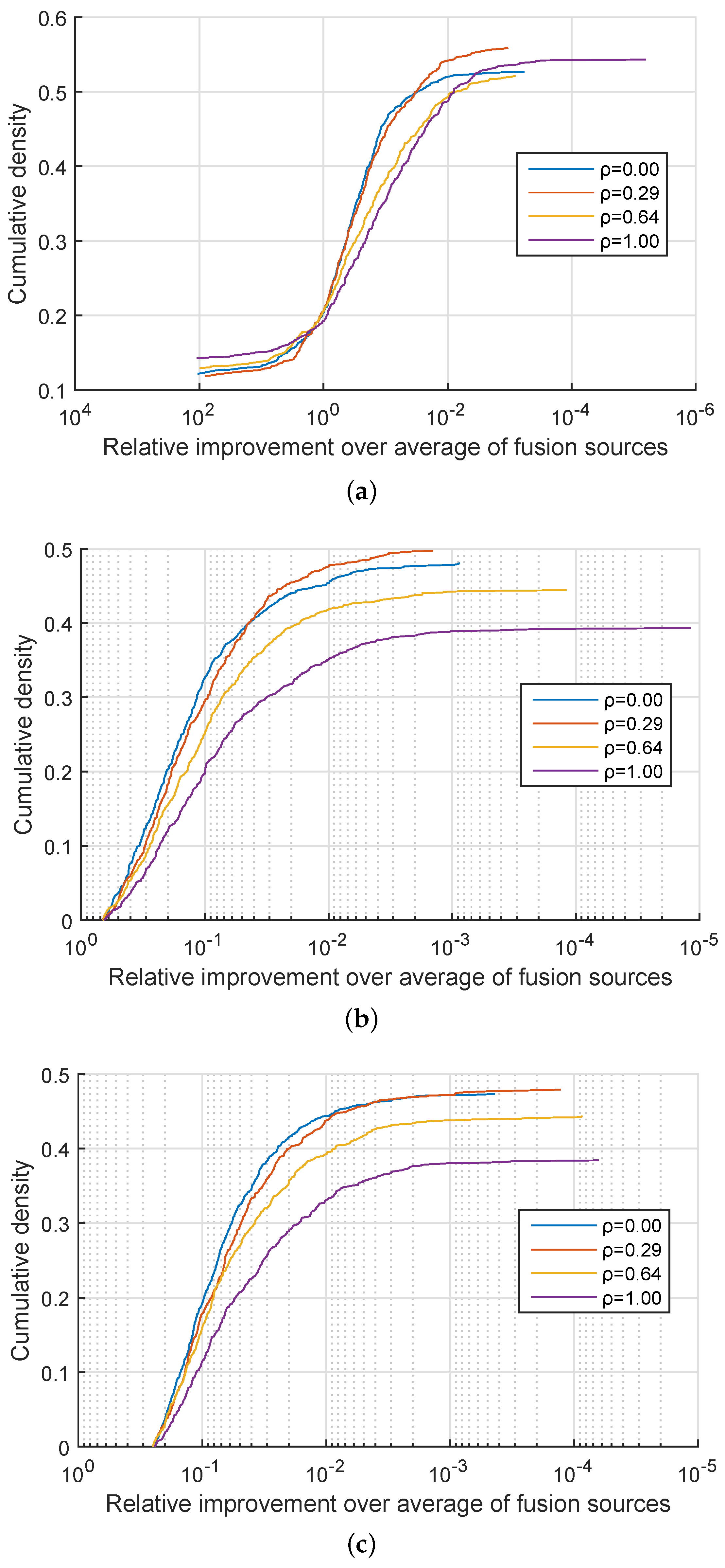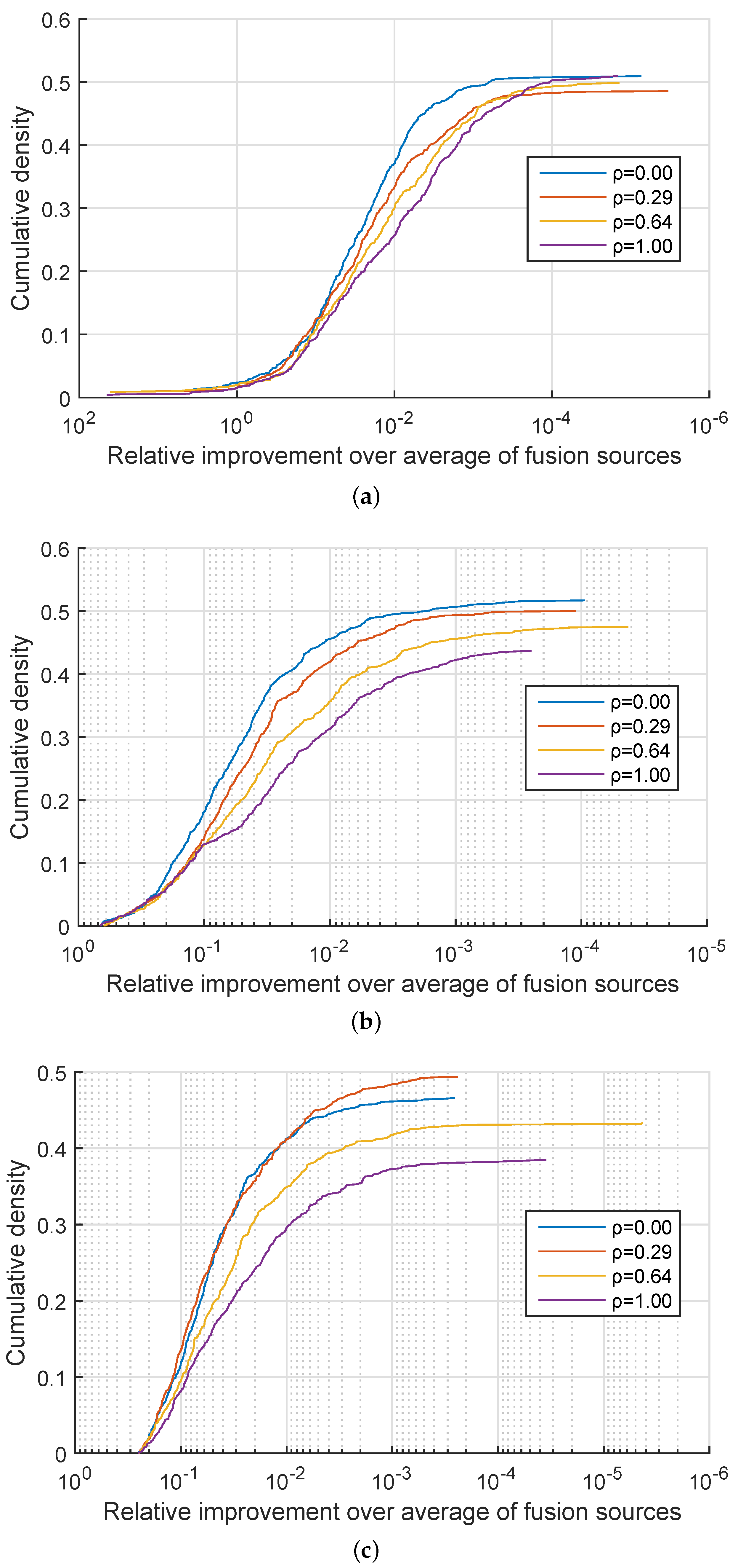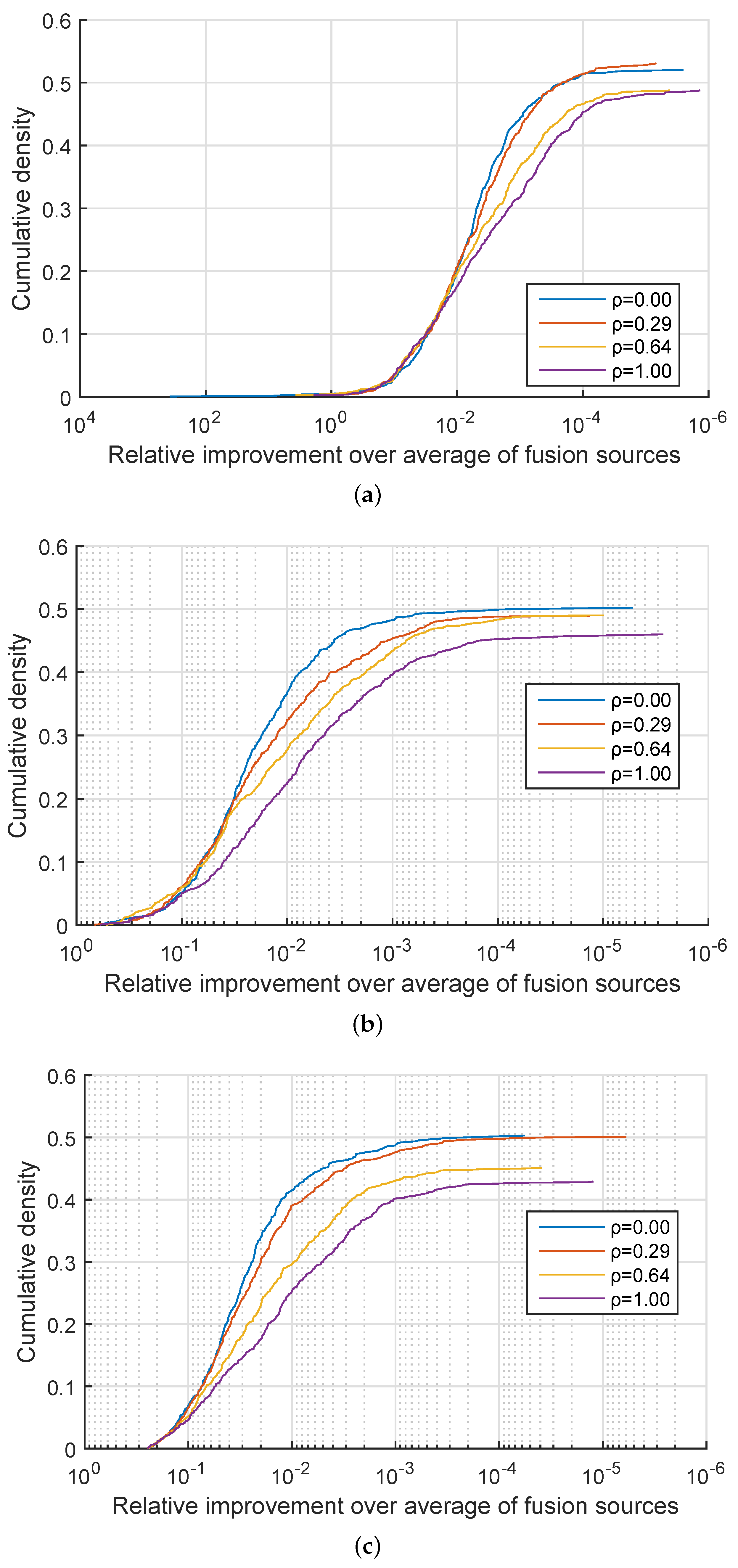In approximately 50% of the cases my method performed equally well as linear fusion and in the remaining 50% of the cases effected an improvement. A more detailed insight is offered by the plots in Figure 1, Figure 2 and Figure 3 which show the cumulative density distribution of the relative improvement achieved by the proposed method, that is $({\partial }_2-{\partial }_1)/{\partial }_1$ when the source was correctly matched, across different experiments. For example from Figure 1 it can be seen that the matching score separation increased twofold (corresponding to the abscissa value of ${10}^0$) in approximately 20% of the cases for the three experiments with ${\beta }_n=0.05$, and in approximately 15% of the cases for the three experiments with ${\beta }_n=0.32$ from Figure 2, while in the three experiments with ${\beta }_n=3.00$ the relative differential matching score increase of this degree was rare (Figure 3). A comparison of the plots in the three figures further reveals that the dissimilarity between information sources has little effect on the average benefit of the proposed method. However the value of $\Delta$ did affect performances for different values of $\rho$. Specifically, across Figure 1, Figure 2 and Figure 3 it can be seen that for small values of $\Delta$, that is, for very similar information sources that we are seeking to discriminate between, the proposed fusion methodology offered approximately equal benefits over linear fusion for different values of $\rho$. In other words the redundancy of the two sensed modalities, or lack thereof, had little effect. In contrast, as the information sources become more separated (increasing $\Delta$), the greater the effect of $\rho$ becomes, with the proposed method offering the greatest advantage when the sensed modalities are complementary i.e., when $\rho =0$.

3.2. Object Recognition

In a controlled experiment using synthetic data and and well-understood information sources, I demonstrated both the superior performance of the proposed generic fusion approach over the common alternative in the form of linear fusion, as well as the consistency of its behaviour with theoretical expectations put forward previously. I next set out to examine whether the same advantages are observed when real-world data is used instead. After all, recall that the central aim of the present paper is to scrutinize the soundness of linear fusion as a generic baseline and argue in favour of the described quadratic mean-based fusion as an alternative with superior performance but paralleled quasi-universality and simplicity of implementation.

My first case-study involves computer-based object recognition. This is an important problem in the spheres of computer vision and pattern recognition, and which has potential for use in a wide spectrum of practical applications. Examples range from motorway toll booths that automatically verify that the car type and its licence plate match the registration database, to online querying and searching for an object of interest that was captured using a mobile phone camera. Object recognition has attracted much research attention [13,14,15,16] and this interest has particularly intensified in recent years after significant advances towards practically viable systems have been made [15,16,17].

Here I consider the fusion of texture-based and shape-based object descriptors. The former group has dominated research efforts to date [17] and has been highly successful in the matching of textured objects. However, it fails when applied on untextured objects (sometimes referred to as ’smooth’) [15] Considering that their texture is not informative, characteristic discriminative information of smooth objects must be extracted from shape instead. Following the method described in [18] I extract and process the representations of the two modalities (texture and shape) independently. An object’s texture is captured using a histogram computed over a vocabulary of textural words, learnt by clustering local texture descriptors extracted from the training data set. Similarly, a histogram over a vocabulary of elementary shapes, learnt by clustering local shape descriptors, is used to capture the object’s shape. I adopt the standard SIFT descriptor as the basic building block of the texture representation and an analogous descriptor of local shape for the characterization of shape [19]. In both cases descriptors are matched using the Euclidean distance.

3.2.1. Results, Analysis and Discussion

As in the preceding section in which synthetic data was used, fused quasi-similarities between the observed data and the two information sources were computed as per (31)–(34), and their performance assessed by analysing the corresponding differential matching scores computed for the correct and incorrect information sources as detailed previously and summarized by (39) and (40).

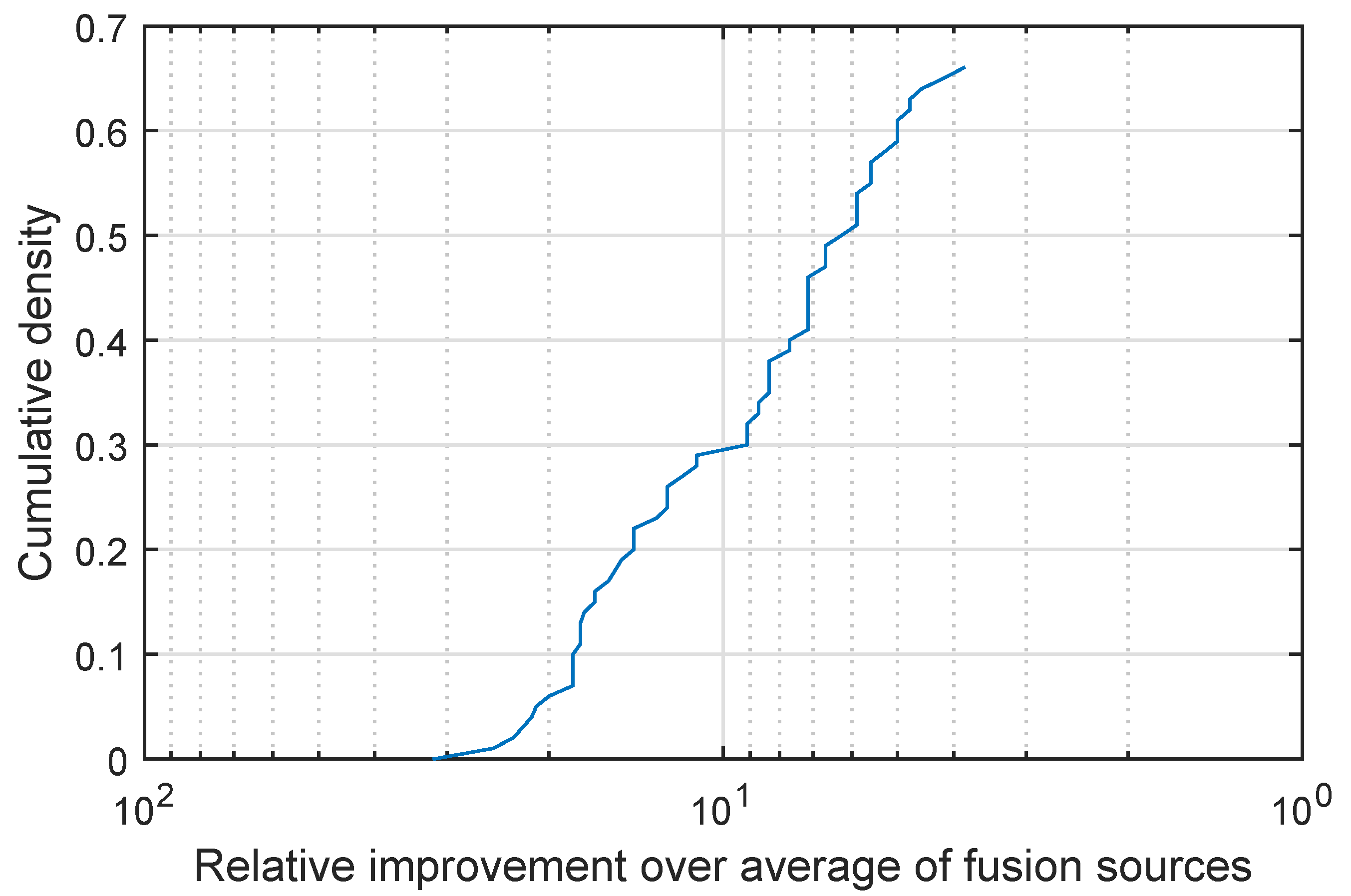
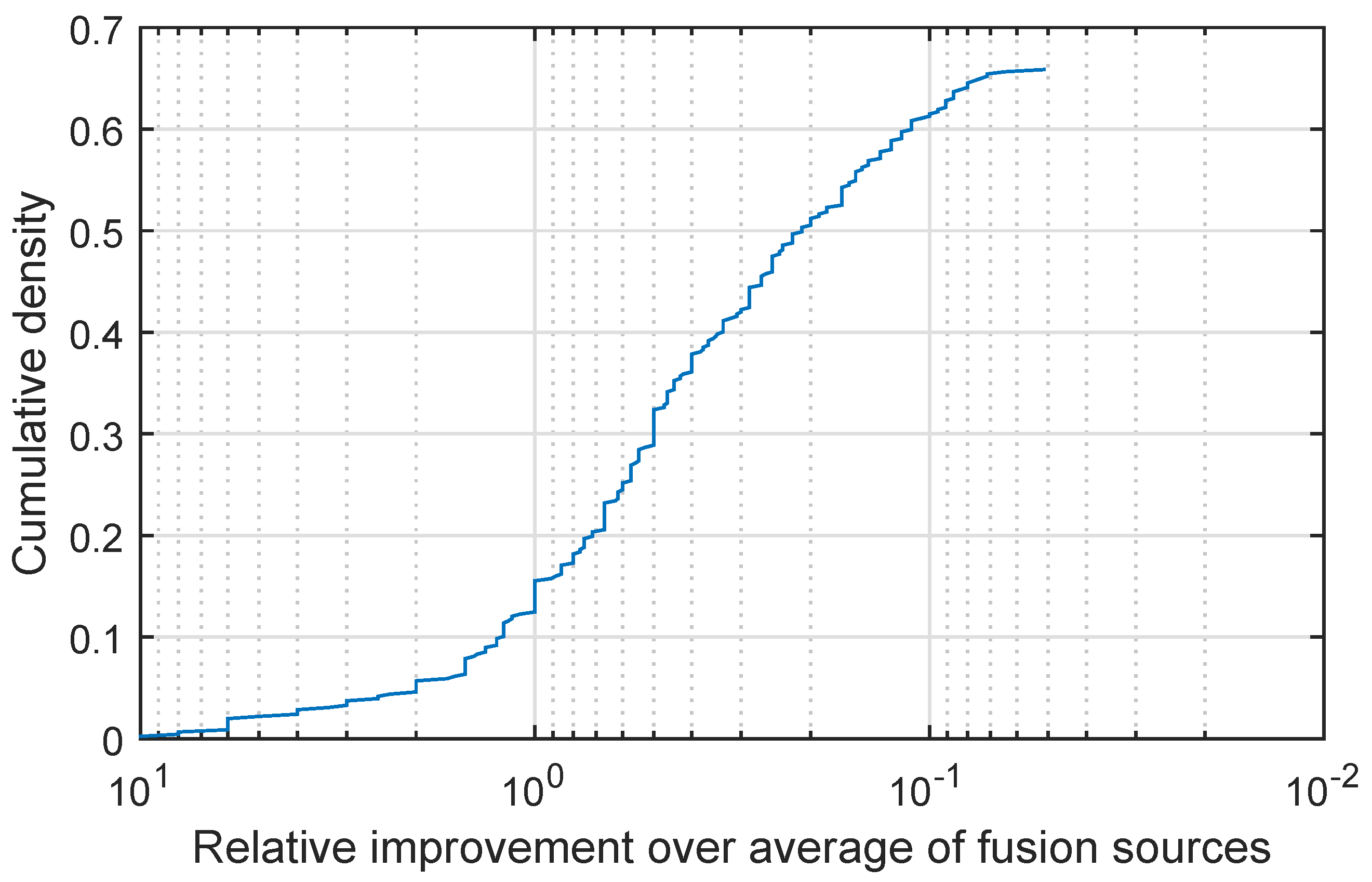
I display my findings in Figure 4 which shows a plot of the cumulative density distribution of the relative improvement achieved by the proposed method (as before please note that the abscissa scale is logarithmic and that it is increasing in the leftward direction). Firstly let us make the highly encouraging observation that the same qualitative behaviour of this characteristic plot is exhibited on this real-world data set as on the synthetic data of the previous experiment. Remarkably, in all cases the proposed fusion strategy did at least as well as the simple weighted fusion. In approximately 66% of the cases the proposed quadratic fusion exhibited superior performance, performing on par in the remaining 34% of the cases. A further examination of the plot reveals an even stronger case for the proposed method—not only does it outperform simple weighted fusion in 66% of the cases but it does so with a great margin. For example in 30% of the cases the inter-class separation is increased 10-fold (i.e., by an order of magnitude).

3.3. Arrhythmia Prediction

My second real-world case-study concerns automatic arrhythmia prediction from demographic data and physiological measurements. This is a challenging task of enormous importance in the provision of timely and informed healthcare provision to the population at risk of cardiac complications. This primarily includes individuals with preexisting cardiac problems or congenital factors, which are further modulated by various environmental factors such as high physical exertion [20] or the use of certain classes of drugs.

A normally functioning human heart maintains a remarkably well controlled heartbeat rhythm. Arrhythmias are abnormalities of this rhythm and are caused by physiological factors pertaining to electrical impulse generation or propagation. Arrhythmia types can be grouped under the umbrellas of three broad categories: tachycardias (overly high heartbeat rate), bradycardias (overly low heartbeat rate), and arrhythmias with an irregular heartbeat rate. While most arrhythmias are transient in nature and do not pose a serious health risk, some arrhythmias (particularly in high risk populations) can have serious consequences such as stroke, cardiac arrest, or heart failure and death [21].

Arrhythmias can be diagnosed using nonspecific means, e.g., using a stethoscope or a tactile detection of pulse, or specific methods and in particular the electrocardiogram (ECG). Moreover, the rich information provided by the latter can be used to predict and detect the onset of arrhythmias by analysing electric impulse patterns [22]. In the present study I evaluate the proposed fusion methodology in the context of this prediction.

I used the dataset collected by Guvenir et al. [22] which is freely available online and can be downloaded [23]. The dataset comprises a rich set of demographic and antropometric variables, such as each person’s age, sex, height, and bodyweight, as well as a variety of features extracted from the person’s ECG, including the heart rate and a series of characteristics of the corresponding signal deflections (the duration of the QRS interval, amplitudes of Q, R, and S waves etc.); please refer to the original publication for full detail [22]. The target variable for the purpose of the present experiment can be considered to be binary valued, taking on the value 0 when arrhythmia is not present and 1 when it is; please see

Table 1. An illustration of the adopted arrhythmia dataset, originally collected and described in detail by Guvenir et al. [22]. It comprises 279 input variables, of which only a small selection is shown here, and the corresponding target variable which for the purpose of the present experiment can be considered to be binary valued, taking on the value 0 when arrhythmia is not diagnosed and 1 when it is.

Age	Gender	Height	Body Weight	QRS Duration	…	Arrythmia
(Years)		(cm)	(kg)	(ms)		(Yes/No)
75	Male	190	80	91	…	Yes
56	Female	165	64	81	…	Yes
…	…	…	…	…	…	…
55	Male	175	94	100	…	No
…	…	…	…	…	…

.

I consider two baseline classifiers. The first of these takes height, bodyweight, and the duration of the QRS interval as input variables (i.e., independent variables). The second one makes the prediction based on what are effectively integrals of Q, R, and S deflections (i.e., referred to as QRSA in the dataset description; please see the original reference for detail [22]), and the Q, R, S, and T deflections (i.e., referred to as QRSTA in the dataset description. Each classifier is built upon a generalized linear model (GLM) [24]. Recall that in a GLM the mean $E\left[Y\right]$ of the target, outcome variable Y is related to a linear predictor based on the independent variables through a link function $\mathcal{L}$:

$$\begin{array}{c}\hfill E\left[Y\right]\equiv \mu ={\mathcal{L}}^{-1}(1+\alpha x).\end{array}$$

(41)

The variance $\mathrm{Var}\left[Y\right]$ of Y is modelled as a function $\mathcal{V}$ of this mean:

$$\begin{array}{c}\hfill \mathrm{Var}\left[Y\right]=\mathcal{V}\left(\mu \right)=\mathcal{V}\left({\mathcal{L}}^{-1}(1+\alpha x)\right).\end{array}$$

(42)

In my experiment, the continuous output of a GLM is used to detect the presence of arrhythmia using what is effectively the nearest neighbour criterion: if the output is closer to 0 the prediction is taken to be negative, and if it is closer to 1 positive. The dataset contains 452 diagnosis cases of which 100 were used for training the classifiers; the remaining 352 were used for testing.

3.3.1. Results, Analysis and Discussion

As in the previous experiments, fused quasi-similarities between the observed data and the two information sources were computed as per (31)–(34), and their performance assessed by analysing the corresponding differential matching scores computed for the correct and incorrect information sources as detailed previously and summarized by (39) and (40).

I display my findings in Figure 5, which shows a plot of the cumulative density distribution of the relative improvement achieved by the proposed method (as before please note that the abscissa scale is logarithmic and that it is increasing in the leftward direction). We can again start with the observation which can be made by comparing the characteristics of the plot in Figure 5 with those of the plots in Figure 4 and Figure 1, Figure 2 and Figure 3 and observing that again the same qualitative behaviour is exhibited on this data too. In all cases the proposed fusion strategy did at least as well as the simple weighted fusion, with approximately 65% of the cases resulting in superior performance of the proposed quadratic fusion and the remaining 35% in on a par performance. As in the previous experiments when my method outperforms simple weighted fusion it does so with a significant margin with an over doubled separation increase in approximately 16% of the cases. Moreover I found that while simple weighted fusion failed to improve the prediction of the better performing baseline classifier in 15% of the cases, the same was the case with the proposed method in fewer than 7.8% of the cases.

3.4. Car Accident Fatality Prediction

My fourth and final experiment concerns the inference of risk factors for car accident fatalities. In particular in this experiment I was interested in discovering what aspects of the context of an accident predict best if a fatality will occur. For this purpose I used the official statistics released by the government of the USA through the Fatality Analysis Reporting System (FARS) for the year 2011. These are freely publicly available and dataset can be downloaded [25]. The dataset comprises a number of person specific variables, such as age, sex, race, blood alcohol level, and drug use status, as well as a variety of variables pertaining to the context of the accident, including the type of the road and the state where the accident took place, and the weather conditions at the time (please see [25] for full description). The target variable for the purpose of the present experiment can be considered to be binary valued, taking on the value 1 when there has been a fatality and 0 otherwise; please see

Table 2. An illustration of the adopted car accidents dataset released by the government of the USA through the Fatality Analysis Reporting System (FARS) for the year 2011. It comprises 15 input variables, of which only a selection is shown here, and the corresponding target variable which for the purpose of the present experiment can be considered to be binary valued, taking on the value 1 when there has been a fatality and 0 when not.

Clear Atmospheric	Driver	Alcohol	Driver	…	Fatalities
Conditions (Yes/No)	Age	Blood Level	Gender		(Yes/No)
Yes	27	0	Male	…	No
Yes	60	0	Female	…	Yes
…	…	…	…	…	…
No	20	0.21	Male		Yes
…	…	…	…	…	…

.

As in the previous experiment, I consider two baseline classifiers, each built upon a generalized linear model. The first of these takes the person’s age and blood alcohol level as input variables (i.e., independent variables). The second one makes the prediction based on atmospheric conditions and the road type. Following the same framework as described in the previous section, the continuous output of a GLM is used to predict the occurrence of a fatality using what is effectively the nearest neighbour criterion: if the output is closer to 0 the prediction is taken to be negative, and if it is closer to 1 positive. The dataset contains 5000 accidents of which 1000 randomly selected cases were used for training the baseline classifiers with the remainder employed for performance evaluation.

3.4.1. Results, Analysis and Discussion

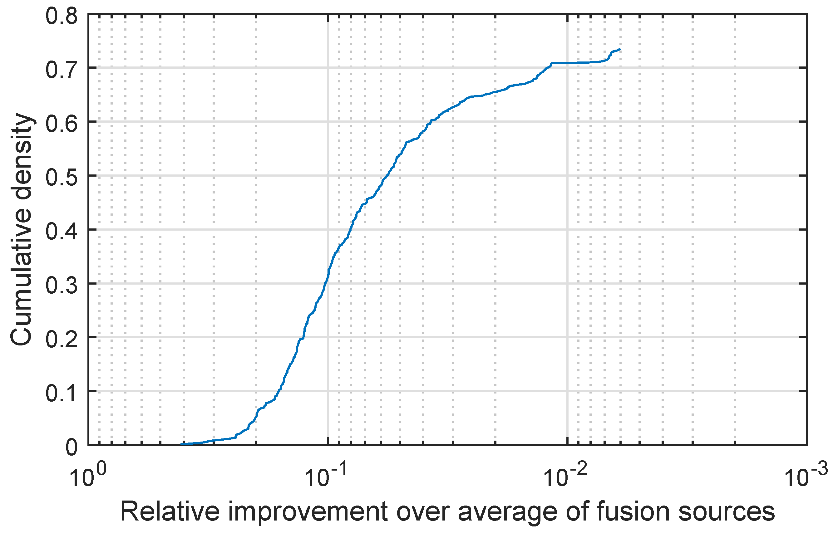
I followed the same evaluation methodology as in the preceding experiments. In the same vein I display my findings in Figure 6 which shows a plot of the cumulative density distribution of the relative improvement achieved by the proposed method (as before please note that the abscissa scale is logarithmic and that it is increasing in the leftward direction). Yet again, in agreement with the results obtained in all experiments I conducted, we can observe the same functional characteristics in the plot of Figure 6 and of those in Figure 1, Figure 2, Figure 3, Figure 4 and Figure 5. In further agreement with the previous experiments is my finding that in all instances of car accidents used for evaluation, the proposed fusion strategy did at least as well as the simple weighted fusion in terms of its predictive ability. With regard to this point, it is interesting to note that notwithstanding the remarkable qualitative similarity of the CDFs corresponding to different experiments, there are some quantitative differences. For example, note that in the present experiment approximately 73% of the cases resulted in superior performance of the proposed quadratic fusion and the remaining 27% in on a par performance. The proportion of evaluation instances yielding superior performance is thus higher than e.g., in the object recognition experiment described in Section 3.2. However, the resulting benefit is smaller. For example, while in the object recognition experiment about 30% of the evaluation cases result in at least 10-fold class separation increase, in the present experiment in no case is the benefit as large. This is most likely a consequence of the inherent information content in the data itself, rather than of some algorithmic aspect of the proposed method. In other words, the lesser advantage (though still consistent and observed in an overwhelming number of cases) of using the proposed method stems from greater redundancy across the fused information sources.

4. Summary and Conclusions

This paper considered the task of designing a score-level fusion methodology which is simple, clear, and generic in its approach, allowing it to be used widely as a reasonable baseline against which novel fusion approaches can be compared. In most cases the existing literature adopts simple weighted linear fusion to this end. I argued that this is not a good choice in that an equally simple but more effective alternative can be formulated in the shape of quadratic mean-based fusion. The argument was founded on theoretical grounds and was further supported using an intuitive interpretation of the derived theoretical results, and lastly demonstrated using a comprehensive series of experiments on a diverse set of fusion problems. The superiority of the proposed fusion approach was first demonstrated using a classification test on synthetically generated data, and then followed by three problems of major research interest: computer vision-based object recognition, ECG-based arrhythmia detection, and fatality prediction in motor vehicle accidents.