Article

Estimating Mangrove Biophysical Variables Using WorldView-2 Satellite Data: Rapid Creek, Northern Territory, Australia

by
Muditha K. Heenkenda
1,*,
Stefan W. Maier
2 and
Karen E. Joyce
3
1
Research Institute for the Environment and Livelihoods, Charles Darwin University, Ellengowan Drive, Casuarina, NT 0909, Australia
2
Maitec, P.O. Box U19, Charles Darwin University, NT 0815, Australia
3
College of Science, Technology and Engineering, James Cook University, P.O. Box 6811, Cairns, QLD 4870, Australia
*
Author to whom correspondence should be addressed.
J. Imaging 2016, 2(3), 24; https://doi.org/10.3390/jimaging2030024
Submission received: 2 June 2016 / Revised: 2 September 2016 / Accepted: 5 September 2016 / Published: 8 September 2016
(This article belongs to the Special Issue Image Processing in Agriculture and Forestry)

Abstract

:
Mangroves are one of the most productive coastal communities in the world. Although we acknowledge the significance of ecosystems, mangroves are under natural and anthropogenic pressures at various scales. Therefore, understanding biophysical variations of mangrove forests is important. An extensive field survey is impossible within mangroves. WorldView-2 multi-spectral images having a 2-m spatial resolution were used to quantify above ground biomass (AGB) and leaf area index (LAI) in the Rapid Creek mangroves, Darwin, Australia. Field measurements, vegetation indices derived from WorldView-2 images and a partial least squares regression algorithm were incorporated to produce LAI and AGB maps. LAI maps with 2-m and 5-m spatial resolutions showed root mean square errors (RMSEs) of 0.75 and 0.78, respectively, compared to validation samples. Correlation coefficients between field samples and predicted maps were 0.7 and 0.8, respectively. RMSEs obtained for AGB maps were 2.2 kg/m2 and 2.0 kg/m2 for a 2-m and a 5-m spatial resolution, and the correlation coefficients were 0.4 and 0.8, respectively. We would suggest implementing the transects method for field sampling and establishing end points of these transects with a highly accurate positioning system. The study demonstrated the possibility of assessing biophysical variations of mangroves using remotely-sensed data.

Graphical Abstract

1. Introduction

Mangrove forests are a dominant feature of many tropical and subtropical coastlines. They have a variety of growth forms, including intertidal trees, palms and shrubs, that often grow in dense stands [1]. Although mangroves form valuable ecosystems along sheltered coastal environments, on the global scale, they are disappearing at an alarming rate [2]. For instance, by 2000, the worldwide mangrove extent has fallen below 15 million ha, down from 19.8 million ha in 1980 [3]. The world has thus lost five million ha of mangroves over twenty years, or 25% of the extent found in 1980. The main reasons for rapid mangrove destruction and land clearings are urbanization, population growth, water diversion, aquaculture, agriculture and salt pond construction.
Land clearings throughout catchments and in urbanized areas can cause an increased volume of water entering watercourses, carrying substances, such as topsoil, chemicals, rubbish and nutrients. These substances deposit on sediments in which mangroves grow. The increased amount of water influences the rate of erosion or deposition of sediments, causing a significant problem for the health of aquatic habitats. Therefore, when sustainable developments are progressing through land clearing, it is necessary to ensure effective mangrove conservation.
To set the balance between mangrove conservation and developments, one of the vital roles of monitoring and ultimately managing mangroves is to create an accurate and up-to-date quantitative analysis of their baseline health parameters. However, assessing mangrove health is not a straightforward task. This is due to the complex structure of forests, their biophysical variations and the interaction between mangroves, soil, water and salinity. Therefore, indirect measures that correlate with the levels of vegetation stresses, such as above ground biomass (AGB), canopy nutrient levels, particularly canopy nitrogen level, and leaf area index (LAI), can eventually be considered.
Most of the conventional methods that have been developed for estimating AGB, LAI and canopy nutrient levels have limitations when extended over space and time. For example, estimating biomass using the allometric method is based on measureable canopy dynamics, such as tree height and diameter at breast height (DBH). Due to the within-stand heterogeneity of canopies, labour-intensive, site- and species-specific field measurements are crucial [4,5,6]. However, field sampling within mangrove forests is challenging. Many mangrove species have complex aerial root systems, which make sampling difficult. Furthermore, mangroves are dense and rather difficult to walk through. Remotely-sensed data addresses the major challenges (especially field sampling) identified with already developed conventional methods that estimate AGB and LAI. Most remote sensing-based approaches are capable of estimating plant biophysical characteristics by reducing the shortcomings of field observations.
There are numerous studies to estimate the biophysical characteristics of vegetation using remotely-sensed data. The key issue is to correlate the intensity of electromagnetic energy absorbed or reflected by the plant (spectral reflectance) with ground measurements of biophysical variables. This spectral reflectance is either measured in situ (using spectrometers) or via airborne or spaceborne sensors. Several studies have found strong correlations between forest biomass or LAI and spectral reflectance values at different wavelengths [7,8]. Eckert [9] and Ahamed et al. [10] summarized different studies that analysed the levels of vegetation greenness in terms of vegetation indices derived from remotely-sensed data for estimating biomass. For example, Anaya et al. [7] and Satyanarayana et al. [11] used the normalized difference vegetation index (NDVI) calculated from red and near infrared wavelengths of remotely-sensed data for estimating biomass. However, compared to other terrestrial vegetation types, little has been adapted to mangroves.
Compared to other terrestrial ecosystems, a few studies associated with field samples and remotely-sensed data for producing thematic maps over mangrove forests can be found [11,12,13,14,15,16]. Clough et al. [17], Green and Clark [18] and Green et al. [14] established a relationship between vegetation indices derived from remotely-sensed data and in situ LAI samples for mangroves. Kamal et al. [15] studied the spatial resolution of satellite images, spectral vegetation indices and different mapping approaches for LAI estimation at Moreton Bay, Australia, and Karimunjawa Island, Indonesia. The study confirmed that the LAI estimation accuracy using remotely-sensed data was site specific and varied across pixel sizes and image segmentation scales. Since there is no recorded study related to the Rapid Creek mangrove forest in Darwin, Australia, the demand still exists for estimating the LAI of mangroves by integrating in situ samples, remotely-sensed data and advanced statistical regression algorithms. To the same extent, we could find only a few studies that mapped AGB of mangroves over a large area. For example, recently, Zhu et al. [16] retrieved mangrove AGB from field data and WorldView-2 (WV2) satellite images. This study tested Sonneratia apetala and Kandelia candel mangrove species and a limited number of vegetation indices for AGB mapping over the study site. The study confirmed the importance of the red-edge band of WV2 satellite image and associated vegetation indices for AGB estimation over other spectral regions. Komiyama et al. [19], Komiyama et al. [5], Fu and Wu [4] and Perera and Amarasinghe [20] derived only a relationship between mangrove canopy dynamics, AGB and vegetation indices. Therefore, testing the possibility of mapping AGB of mangroves over a large area from remotely-sensed data is still required.
This study aimed to quantify the spatial distribution of LAI and AGB of mangroves using field measurements and WV2 satellite images. To achieve this aim, the study compared two different spatial resolutions of WV2 data (original spatial resolution of multispectral bands (2 m) with resampled multispectral bands (5 m)) and partial least squares regression algorithm for mapping LAI and AGB variations over a large area.

2. Data and Methods

2.1. Study Area

The Rapid Creek mangrove forest in Darwin, Northern Territory, Australia, was selected as the test site for this study (Figure 1). This area is dominated by five different mangrove species: Avicennia marina, Ceriops tagal, Bruguiera exaristata, Lumnitzera racemosa and Rhizophora stylosa [21]. Other species do not represent significant coverage to be considered separately.

2.2. Field Sampling, Satellite Data and Predictor Variables

A total of 29 plots, 5 m × 5 m in extent, were identified in the field. These plots were selected with trees having similar characteristics (species, age, height and DBH) to represent calculated values accurately. Each of them was oriented in a north-south and east-west direction in order to locate them easily in the satellite image. Inside each plot, five trees were selected to take measurements based on their ability to be identified in satellite images; that is isolated and without clumping to neighbouring tree crowns. A sampling pattern was determined considering the accessibility, density of mangrove forest, mangrove greenness and species variation. Attention was also given to avoid areas close to water features due to the danger of salt water crocodiles that inhabit the region.
Tree height, diameter at breast height and species were recorded. Species were identified based on the guidelines provided by Duke [22] and Wightman [23]. The positions of each the tree and the four corners of each plot were recorded using the non-differentially-corrected Global Positioning System (GPS). Apart from the GPS measurements, we collected some additional measurements to support positioning field plots in the image. These measurements especially refer to distances to closest roads, water features and other features that can easily be identified in the image.

2.2.1. Remotely-Sensed Data and Predictor Variables

An overlapping pair of WV2 satellite images acquired on 26 July 2013 was used as the remotely-sensed data for this study. The main reason for having an overlapping pair of images was to prepare a stereo model of the area to manually extract individual tree crowns. The satellite image capture coincided with the field data acquisition. The satellite is in a nearly circular, Sun-synchronous orbit with a period of 100.2 min. The spatial resolution of multispectral bands was 2.0 m, and the panchromatic band was 0.5 m. Table 1 shows the detailed spectral band description of WV2 images.
WV2 images were radiometrically corrected according to the method described by Heenkenda et al. [21]. First, digital numbers were converted to at-sensor-radiance values, and then, they were converted to top-of-atmosphere reflectance values. The dark pixel subtraction technique in ENVI 5.0 software was applied to remove the additive path radiance. Finally, images were geo-referenced using rational polynomial coefficients provided with the images and ground control points extracted from digital topographic maps of Darwin, Australia. The georeferenced surface reflectance values were used for further analysis.
Non-mangrove areas of images were masked as per Heenkenda et al. [21]. Class-specific rules were developed based on the contextual information from the WV2 images, geometry and neighbourhood characteristics of objects at different hierarchical levels to separate mangrove coverage only (see Heenkenda et al. [21] for a detailed description).
Plant growth is correlated with the expansion of leaf canopy and the increasing weights of woody elements. Hence, the AGB and LAI of mangroves can relate to vegetation indices derived from remotely-sensed data. To take the maximum advantage of the relatively narrow spectral bands of WV2 multispectral images, this study selected nine vegetation indices and the green, yellow, red, red-edge, NIR1 and NIR2 bands of the WV2 image to predict LAI and AGB over the study area (Table 2). These narrowband greenness indices use spectral reflectance values in the red, red-edge, NIR1 and NIR2 regions, and they produce a measure of the photosynthetic characteristics of vegetation. Hence, narrowband greenness indices are more suitable measures of the biophysical variations and vigour of green vegetation than broadband greenness vegetation indices. Vegetation indices shown in Table 2 were calculated for predicting AGB and LAI from WV2 data. Then, spectral bands of the WV2 satellite image and vegetation indices were stacked together to form one image with multiple layers (15 layers) for further processing.
The WV2 multispectral bands were resampled to a 5-m spatial resolution using the cubic convolution resampling method. This was done to simulate remote sensing images from other satellite missions that provide multispectral images within the same spectral region, such as RapidEye. The number of band ratios and vegetation indices was calculated as explained in Table 2. The green (506 nm–586 nm), red (624–694 nm), red-edge (699 nm–749 nm), NIR1 (765 nm–901 nm) and NIR2 (856 nm–1043 nm) bands of the WV2 image and the calculated band ratios and indices were stacked together to form a single image with 15 bands of a 5-m spatial resolution for further processing.
An overlapping panchromatic image pair was oriented to ground coordinates following the digital photogrammetric image orientation steps in the Leica Photogrammetric Suite (LPS)/ERDAS IMAGINE software to obtain a stereo model of the area. The rational polynomial coefficients (RPC’s) calculated during the image acquisition and ground control points extracted from the digital topographic map of Darwin, Australia (scale of 1: 10,000), were used as references. Further, the quality of the stereo model was assessed by comparison with ground control points. Then, outlines of the mangrove field plots that were assessed in the field were digitised using a stereo model. To identify the four corners of field plots in the image, the GPS locations, as well as the indirect measurements that were collected during field sampling were used. To calculate the corresponding predictor variable values of each plot, all pixels within a field plot polygon were considered. However, pixels that represented less than 70% in extent within a plot were discarded from further calculation.
The study selected the digital cover photography method developed by Macfarlane et al. [30] for calculating the LAI of field sampled mangrove trees. Since mangroves are densely clustered with muddy soil underneath the canopy cover, the digital cover photography method is more reliable than plant canopy analysers or area meters (LAI-2200C, LI-3100C, LI-COR 6400, etc.). Vertical photographs of the canopy, pointing the lens of the camera upwards, were taken using a Panasonic Lumix DMC-FT2 compact digital camera. Two levelling bubbles were attached to the camera to ensure that photographs were taken without a tilt. The camera was set to an aperture priority-automatic exposure mode. Due to the densely-clustered nature of mangroves, it is impossible to isolate one tree and take photographs that represent its canopy area. Therefore, 16 evenly-spaced photographs were taken within each plot. The number of trees within the plot was counted.

2.2.2. Estimating the Leaf Area Index

According to Macfarlane et al. [30], vertical photographs were used to estimate the large gaps between mangrove trees, small gaps within mangrove trees, the proportion of the ground area covered by the vertical projection of foliage and branches, the crown cover, the crown porosity and the woody-to-total area ratio of each sampling plot. A detailed description of the method to estimate LAI using digital photographs can be found in Macfarlane et al. [30], Pekin and Macfarlane [31] and Heenkenda et al. [32].
All digital photographs were classified using eCognition software for further calculations. By considering the contrast between vegetation and the background (the sky) of the photographs, areas with higher blue reflectance values were classified as sky. The ratio between the reflectance of blue and red bands was further considered to separate the background and the vegetation. The background was further classified into large gaps (gL) between tree crowns and total gaps (gT), considering the relation to neighbouring features. For example, if the area of the gap is less than 50 pixels and it is surrounded by vegetation, it is classified as a small gap within a tree. Finally, a total number of pixels for large gaps and small gaps was summed to obtain gT (see Heenkenda et al. [32] for the detailed description).
Vegetation was further classified into leaf area and branches/stems. The greenness values were used to identify branches/stems from vegetation. Hence, the greenness was calculated from photographs using Equation (1) [33].
Greenness = 2 × G B R
where G, B and R represent the reflectance (intensity levels) recorded with the green, blue and red bands of the digital camera.
The fraction of foliage cover (ff) that is the proportion of the ground area covered by the vertical projection of foliage and branches [30,31,34] and the crown cover (fc) were calculated as Equations (2) and (3).
f c = 1   g L / Pixels
f f = 1 g T / Pixels
where gL is the total number of pixels of large gaps (gaps between tree crowns), gT is the total number of pixels of gaps, fc is the crown cover, ff is the fraction of the foliage cover and Pixels is the total number of pixels of the photograph.
Considering these results, the crown porosity (ф), which is the proportion of the ground area covered by the vertical projection of foliage and branches within the perimeter of the crowns of individual plants, was calculated from the Equation (4):
ф = 1   f f f c
where ff is the fraction of the foliage coverage and fc is the crown cover.
The effective plant area index (Lt) includes the contribution from woody elements to the total plant cover. Hence, it provides an overestimation for leaf area index [30]. The effective plant area index was estimated using the modified version of the Beer–Lambert law as specified in Equation (5).
L t = f c × ln ( ф ) k
where fc is the crown cover; ф is the crown porosity; and k is the canopy extinction coefficient.
As Perera et al. [35] suggested, the canopy extinction coefficient (k) was taken as 0.5 for this study. This represents the average value of already published k values for mangroves around the world. The factor k mainly depends on stand structure and canopy architecture; therefore, different vegetation types have different values. For example, Breda [36] reviewed k values for forest stands with broad leaves and found a range of values from 0.42 to 0.58. Macfarlane et al. [30] assumed k =0.5 for eucalypt forests. Finally, we calculated the woody-to-total area ratio (α) and the actual leaf area index (LAI) from Equations (6) and (7) [37,38].
α = ( Area B ) ( Area V )
LAI =   L t × ( 1 α )
where ( Area B ) is the total area of branches, except leaves; ( Area V ) is the total area of vegetation including branches; and Lt is the effective plant area index.
The final results represented an actual LAI of individual plots or a cluster of trees. This was then divided by the number of trees to get a value per tree.

2.2.3. Estimating the Above Ground Biomass

The study selected the allometric method for estimating AGB from field measurements. The basic theory of the allometric relationship is that the growth rate of one part of the organism is proportional to that of another [5], and therefore, it depends on measurable canopy dynamics, such as tree height and DBH. Once the regression relationship between canopy dynamics is established, the regression equation estimates the standing biomass of a tree. However, allometric relationships for mangroves are species and site specific [5]. Therefore, special attention was given to use allometric equations developed for mangrove species in Northern Australia or Southeast Asia. Since there was no equation derived for Sonneratia alba and Excoecaria agallocha var. ovalis, the common equation developed by Bai [39] for mangroves in the Northern Territory, Australia, was used (Table 3).
The logarithmic transformation of DBH values was calculated using Microsoft Excel software. Equations from Table 3 were used to calculate Log10 (Biomass). Finally, the calculated above ground biomass values were converted to AGB per square meter (unit = kg/m2) considering the extent of each plot.

2.3. Predicting LAI and AGB

Multivariate regression methods are some of the most-widely used methods for estimating plant biophysical and biochemical variables, in particular for developing empirical models of variables of interest based on satellite image data. Among them, partial least squares regression (PLSR) receives much popularity, as it has been designed to outperform the problems of collinearity of prediction variables and over-fitting with relatively few samples. Hence, PLSR is suitable when the number of predictor variables is large and they are highly collinear [26,42,43]. This study selected the PLSR algorithm to model the relationship between field samples and satellite data. The “pls” package in R software [44] was used for the calculation.
In its simplest form, PLSR specifies a regression model by projecting the predictor variables and response variables to a new space. That is, data are first transformed into a different and non-orthogonal basis similar to a principal component analysis, and the most important partial least square components are considered for building a regression model. Hence, the PLSR procedure extracts successive linear combinations of partial least square factors or components. Once the optimal number of partial least square components is selected, the relationship can be predicted over a large area. A detailed description of the PLSR algorithm is available in Mevik and Wehrens [44], Hastie et al. [45] and Wang et al. [43].
The PLSR algorithm performs best with normalized data without outliers [45]. Therefore, the LAI sample data were normalized with the mean equal to zero and the variance equal to one and analysed for outliers. The mangrove field plot polygons were considered to extract predictor variable values from all pixels within plots, as described previously for a 2-m spatial resolution. Finally, these sampled pixels were randomly divided into two sets: training (70% of sample data) and validation (30% of sample data). By using the “pls” package, the optimal number of components for the prediction or predictive abilities of the model was assessed considering the prediction root mean square error (RMSEP). To obtain RMSEP, the model was internally cross-validated using the leave-one-out cross-validation method with training data. Once the optimal number of components was selected, the model was used to predict LAI over the study area using the “raster” package in R software [46]. Finally, we de-normalized the raster maps considering the mean and variance of the original field samples to obtain real LAI values. A low pass filter (3 × 3 kernel) was applied to smooth data by reducing local variation and removing noise. This process was repeated to analyse the spatial variation of LAI over the Rapid Creek mangrove forest with predictor variables of a 5-m spatial resolution.
Field samples of log-transformed AGB values (allometric equations directly calculated log-transformed AGB) were analysed for the normality and outliers. Then, the above process was repeated to predict AGB over the study area. The sampling plot polygons were considered to extract predictor variable values from all pixels within plots.

2.4. Accuracy Assessment

The accuracies of models were internally assessed using a leave-one-out cross-validation method with training samples at all instances. However, the accuracy of the predicted LAI and AGB maps was assessed using validation data. Approximately one third of field samples of LAI and AGB separately was considered as the validation data (randomly selecting 30% of the sampling pixels within field plots). Root mean squared errors (RMSE’s) and correlation coefficients (r) between predicted values and field measurements were recorded.

3. Results

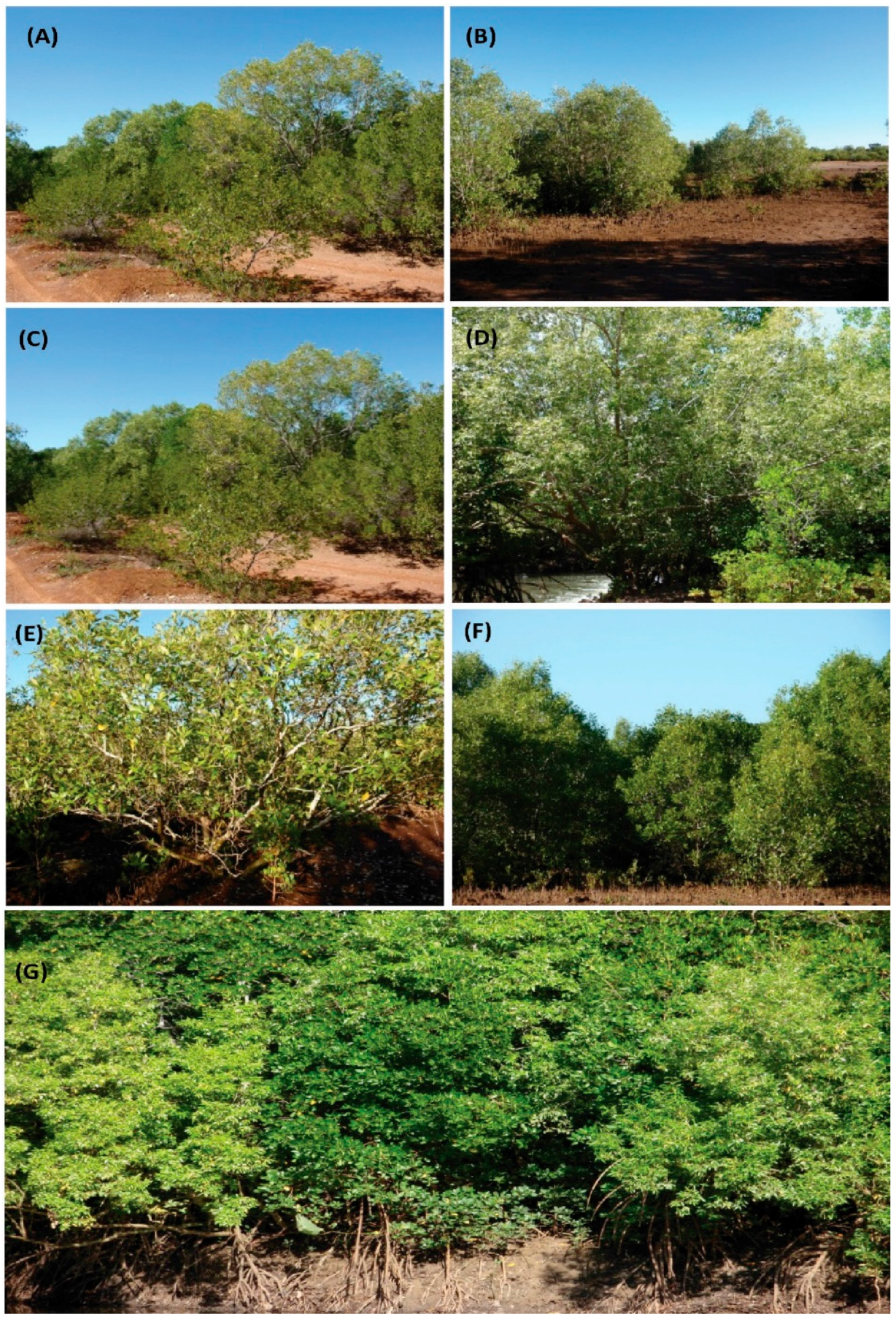
The locations of field plots are shown in Figure 1. Three field plots at the northeast corner of the study area have low biomass values. Their DBH values vary from 1.5 cm to 3.5 cm, and tree heights vary from 1.4 m to 3.6 m. Figure 2A–C shows mangrove trees in these areas. They are newly-regenerated, small trees. Some areas are covered with large, wide-spread, multi-stemmed mangrove trees (Figure 2D,E). Their DBH values vary from 10.0 cm to 19.0 cm, and heights range from 4.0 m to 8.0 m. There are some areas especially near water features covered by densely-clustered mangroves with different heights (Figure 2F,G).
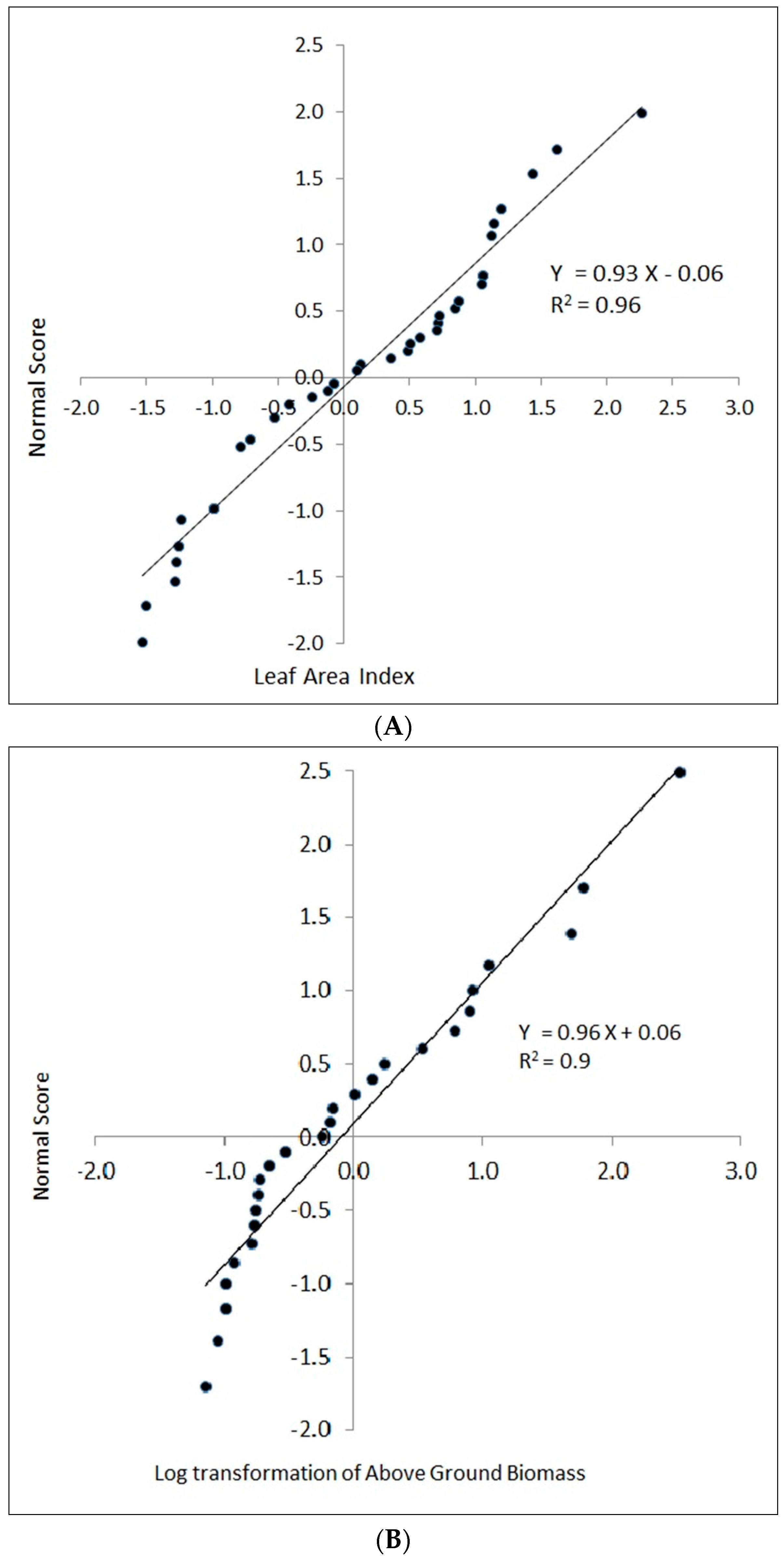
The normal score plot of field samples is shown in Figure 3. The normal score represents alternative values to data points within a dataset that would be expected from a normal distribution. Points on the reference line are closer to normality, and horizontal departures indicate departures from normality. Hence, few sampled mangrove trees were removed from further calculations, as they exhibited non-normality with extremely low or high values (Figure 3A,B). The normality was measured with respect to the coefficient of determination of regression (R2). The R2 of LAI equals 0.96, and the log-transformed AGB showed 0.9. Once outliers were removed, the remaining field samples were normally distributed.

3.1. Predicting AGB and LAI

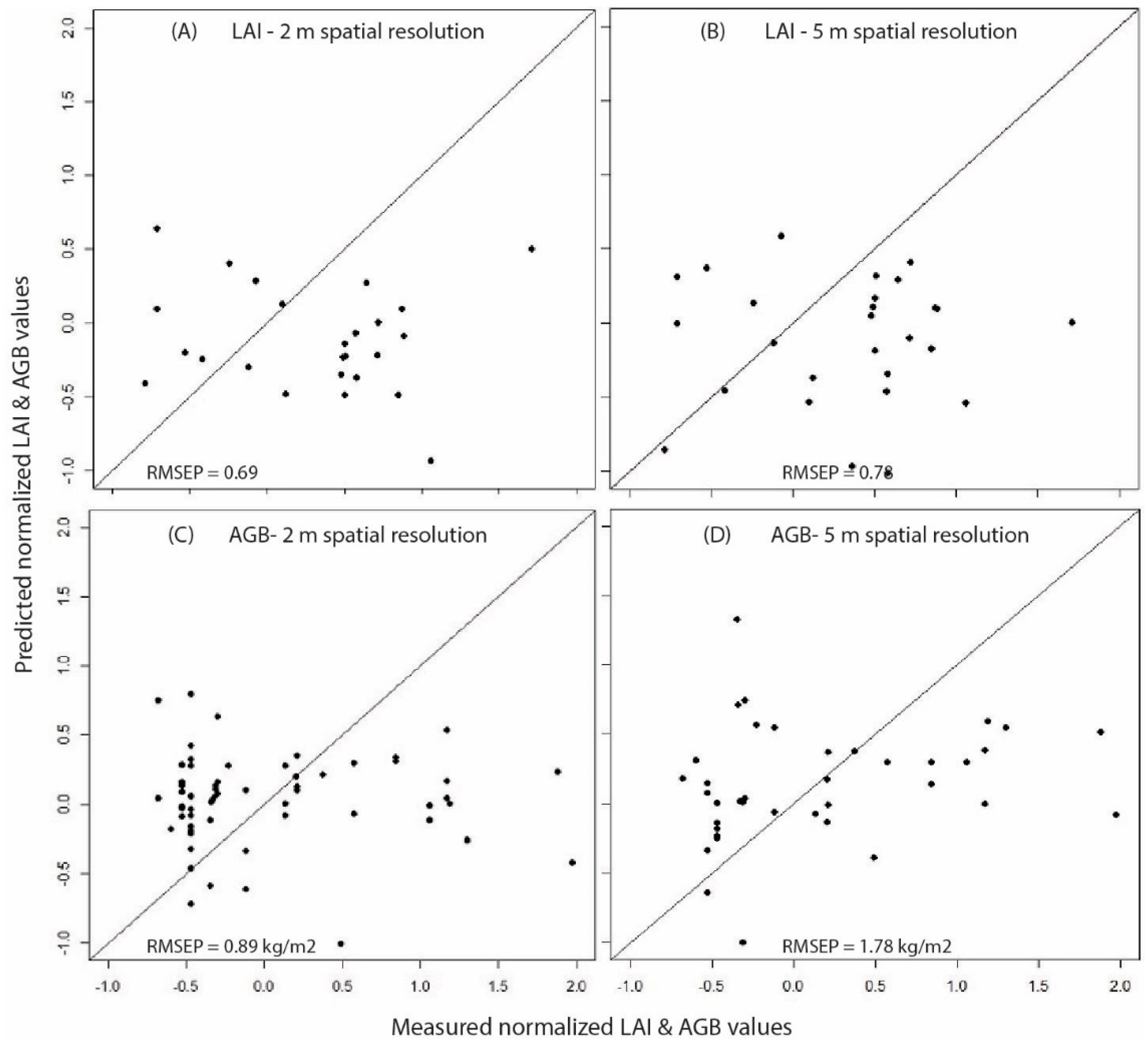
A number of studies indicated PLSR as a powerful tool to extract spectral signatures and to create reliable models of LAI [25]. The performance of the PLSR model: a “goodness of fit” is represented by a root mean squared error of prediction (RMSEP). The RMSEP of the PLSR for LAI prediction was 0.69 with four components when considering a 2-m spatial resolution. This value confirmed a good relation between predictor variables and LAI field samples. Therefore, four components with all predictor variables were used for final mapping. The RMSEP of a 5-m spatial resolution was 0.78 with six components. Six components with all predictor variables were used for final mapping. If the prediction model is perfect, the RMSEP and RMSE (the root mean squared error for training and validation data) should be very similar. However, the RMSE values of LAI map with a 2-m and a 5-m spatial resolution were 0.75 and 0.78, respectively (Table 4). Although the slight difference with respect to a 2-m spatial resolution shows model overfitting, the model performance for 5-m spatial resolution data was good.
Figure 4A–D shows the cross-validated predictions with selected components versus measured values (or field samples). Most of the points (normalized LAI and AGB values) slightly deviate from the aspect ratio = 1 line. However, there is no indication of a curvature or other anomalies. The validation results (RMSEP) are shown in Figure 4.
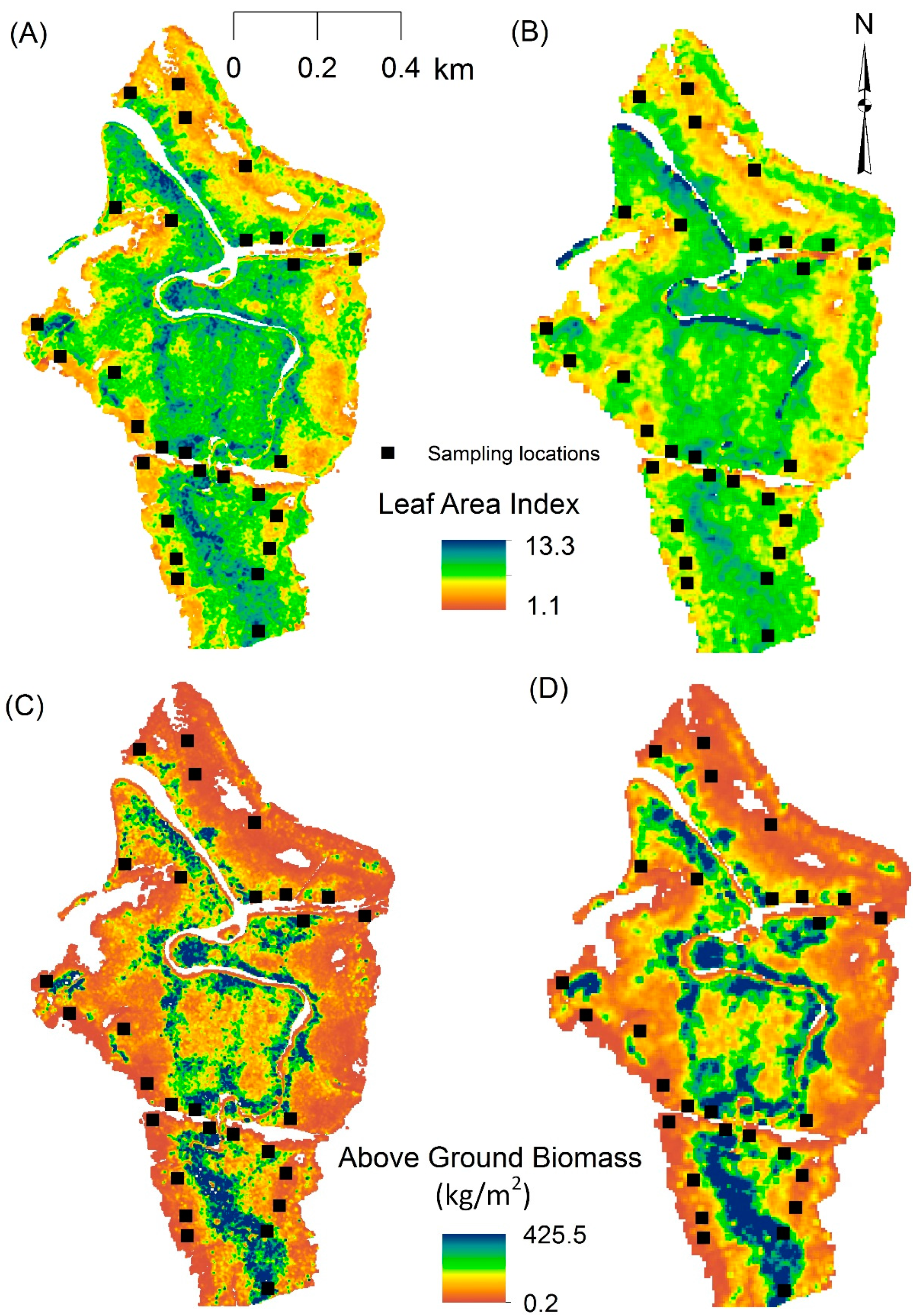
The predicted LAI map with a 2-m spatial resolution is shown in Figure 5A. The highest LAI value is 13.0, and the lowest one is 0.2. The mean LAI value is 3.9 with a standard deviation of 1.1. Approximately 70% of data ranged from 0.8 to 4.5. Although LAI values are normally distributed, the pattern has a high dispersion. The majority of data values are between 0.8 and 4.5. LAI values are high where closer to edges of water features. The upper right side of the map (Figure 5A) shows low LAI values, and this area is dominated by relatively small recently re-generated mangrove plants.
The predicted LAI map with a 5-m spatial resolution is shown in Figure 5B. The highest LAI value is 13.3, and the lowest one is 1.1. The mean LAI value is 4.2 with a standard deviation of 0.8. More than 70% of LAI values are between 3.2 and 4.8 showing a normal distribution. However, LAI values are high where closer to edges of water features. The upper right side of the map (Figure 5B) shows low LAI values, as shown in the map with a 5-m spatial resolution (Figure 5B).
When comparing Figure 5A,B at this scale, it can be seen that results obtained from 2-m spatial resolution images provide finer LAI spatial variations than results from 5-m spatial resolution images. However, at a larger scale, Figure 5A shows scattered LAI variation patterns. These patterns do not correctly represent the spatial variations of mangrove trees around those areas and, thus, the spatial distribution of LAI of the area.
The visual appearances of the AGB maps are in-line with the field observations. Most of the areas having low AGB values are dominated by relatively small and young mangrove trees. For instance, three field plots at the northeast corner of the study area (Figure 1) have low biomass values. The average measured DBH in this area was 1.8 cm, and the average height of mangrove trees was 1.6 m. Mangrove trees are dense and tall along the water features, and these areas showed high AGB values.
When considering the performance of the PLSR model for AGB, the RMSEP for a 2-m spatial resolution was 0.89 kg/m2; however, once predicted AGB over the study area, the RMSE was 2.2 kg/m2. The correlation coefficient obtained with respect to validation samples was 0.4 (Table 4). Hence, it can be concluded that the model was over fitted. The RMSEP for a 5-m spatial resolution was 1.7 kg/m2, and the RMSE with respect to validation data was 2.0 kg/m2 with strong linear correlation between predicted and sampled AGB values.
The predicted AGB values with a 2-m spatial resolution ranged from 0.12 kg/m2 to 425.5 kg/m2 with a mean value of 22.5 kg/m2 and a standard deviation of 8.1 kg/m2 (Figure 5C). AGB values with a 5-m spatial resolution ranged from 0.12 kg/m2 to 423.2 kg/m2 with mean value of 18.4 kg/m2 and a standard deviation of 7.2 kg/m2 (Figure 5D). At both instances, the AGB values showed a skewed distribution rather than a normal distribution. The majority of the data (more than 70%) were in between 30 kg/m2 and 267 kg/m2. The main reason should be the extremely large, multi-stemmed Avicenna marina and Rhizophora stylosa mangrove trees in this forest. They were spread over a large area without secondary forest underneath. The highest measured, as well as highest predicted AGB values represent these areas (423.2 kg/m2 and 425.5 kg/m2).

3.2. Accuracy Assessment

The RMSE values with respect to the validation samples and correlation coefficients between predicted values and validation samples were recorded (Table 4). We used randomly-selected, approximately one third of field samples as the validation samples for both instances. Although the AGB map with a 2-m resolution showed low linear correlation between predicted values with validation samples, the LAI map showed a good correlation. AGB and LAI maps with a 5-m spatial resolution showed a strong linear correlation between predicted values and validation samples.

4. Discussion

The major advantage of assessing AGB and LAI from remotely-sensed data is the estimation of AGB and LAI over large areas without having extensive field campaigns. This is also a solution for many logistical and practical problems arising with field efforts. For example, access to interior extremely-dense mangrove patches is extremely difficult. In addition, the methods are non-destructive, relatively fast and economical with less labour force.

4.1. Predicting LAI

Mangrove canopies are densely clustered with overlaps. Extended root systems and muddy soil underneath the canopy cover make it difficult for sampling. Although the widely-accepted method for LAI estimation is the simulation of canopy light profiles using conventional instruments, such as portable plant canopy analysers or area meters, the digital cover photography method is more reliable than conventional instruments for mangrove forests. The digital cover photography approach is independent from the radiation condition of the forest and can be used for an extensive sampling. This method was later tested for types of cameras, digital file compression, image size and ISO equivalences, and little or no effect on estimating LAI was found [31]. Lui and Pattey [33] also recommended using the digital cover photography method by comparing its results with LAI estimation from conventional equipment.
The mean value of the predicted LAI map with a 2-m spatial resolution (3.9) is slightly lower than previously-recorded mangrove studies around the world. For instance, Clough et al. [17] estimated the LAI of Rhizophora apiculata mangrove forest in Malaysia using three different methods and obtained mean LAI values: 4.9, 4.4 and 5.1. LAI of Avicennia marina plantations in Thailand varied from 0.5 to 5.0. For the homogeneous mangrove stands at Moreton Bay, Australia, LAI values ranged from 0.26 to 3.23 with 1.97 as the mean value [15]. Kamal et al. [15] also assessed heterogeneous mangrove stands at Karimunjawa Island, Indonesia, and obtained LAI values from 0.88 to 5.33 (mean value = 2.98). A remote sensing study on LAI in the British West Indies showed a range from 0.8–7.0 with 3.96 as the mean. Statistics from the predicted LAI map of this study with a 5-m spatial resolution (4.2) was as close as previous mangrove studies. However, comparing results from this study with other studies is not a perfect approach to make a conclusion regarding the spatial distribution of LAI. They are site and species specific. When looking at cross-validated predictions, most of the predicted LAI values are lower than field sample values (Figure 4A,B). One consideration is the canopy extinction coefficient (k) used to calculate Lt. Although the used value (0.5) represents the average of already published k values for mangroves around the world, this might not be the correct value for this area. Further, LAI values vary with the spatial resolutions of remote sensing images used for data processing. Kamal et al. [15] recently confirmed that the accuracy of LAI estimation was site specific and depends on the pixel size of the remotely-sensed images, and their study even indicated two different LAI distribution patterns for homogeneous and heterogeneous mangrove forests.
The performance of the PLSR model: a “goodness of fit” is represented by a root mean squared error of prediction (RMSEP). The accuracy of the predicted maps was assessed using the root mean squared error (RMSE) compared to the validation samples. If the prediction model is perfect, RMSEP and RMSE (the root mean squared error for training and validation data) should be very similar. However, in this study, values related to a 2-m spatial resolution are slightly different, indicating a model overfitting. The best model performances were shown when using a 5-m spatial resolution. According to Zheng and Moskal [47], the accuracy of LAI estimation depends on two main reasons: overlapping and clumping between leaves within canopies due to the non-random distribution of foliage and light obstruction from canopy branches, trunks and stems. The first reason relates to this study, as well, due to mangrove canopy overlapping. The latter will not be a problem because of using vertical photographs rather than simulating light transmission. Another reason for obtaining low accuracies with a 2-m spatial resolution than a 5-m spatial resolution would be the spatial mismatch between field samples and predictor variables due to positional errors.
To establish the relationship between field samples and predictor variables, a corresponding predictor pixel value for each field sample should correctly be extracted. Hence, the positional accuracy of field samples and the pixel size is important. Laongmanee et al. [48] assessed the optimal spatial resolution for estimating the LAI of Avicennia marina plantations in Thailand. The best results were produced by satellite images with a 10-m spatial resolution. Although there is still room to confirm this finding, Green and Clark [18] suggested analysing the information of satellite data within a 5 m × 5 m block of pixels regardless of the spatial resolution for LAI estimation. Green and Clark [18] also argued that although high resolution satellite data provide significantly greater levels of accuracy, they were not capable of fixing positional errors. Hence, it is clear that the satellite data with a 2-m spatial resolution are not suitable to establish this match-minimizing effect from the positioning errors. According to this study, although 2-m or 5-m spatial resolutions can interchangeably be used for mapping LAI in the Rapid Creek mangrove forest, we would recommend testing a 5 m × 5 m block of pixels regardless of the spatial resolution for LAI estimation, as suggested by Green and Clark [18]. Further, we would recommend using the transect method for field sampling to minimize positional errors. Two ends of transects can be established outside the mangrove forest with DGPS (differential GPS). Then, all other measurements can be based on the established transect line with greater accuracy.

4.2. Predicating AGB

We used allometric equations for AGB calculation. Allometric relationships are highly species specific and less site specific [5,19]. Although special attention was given to using allometric relationships that were specifically developed for Northern Territory, Australia, mangrove species, we used some equations that were developed for Northern Queensland, Australia, and Sri Lanka. In this study, it was not possible to use the common equation proposed by Komiyama et al. [19], as it requires the vegetation density, which we did not measure in the first place. Therefore, for the mangrove species for which we could not find already developed allometric equations, we used a generic equation developed by Bai [39] for the Northern Territory, Australia, mangroves.
Some of the sampled Avicennia marina and Rhizophora stylosa species are multi-stemmed mangrove trees. As explained by Clough et al. [49], when there are multi-stemmed mangrove trees, each branch should be treated as a discrete tree, and the dry weight of the common butt should be included to obtain a robust AGB of the tree. However, this discrepancy is important if the consideration is to calculate the AGB of different woody parts of trees only, rather than total AGB [49]. Hence, in this study, we treated each branch of multi-stemmed mangrove trees as a separate tree. The dry weight of the common butt was neglected.
The predicted AGB maps are approximately in-line with visual field observations and AGB calculations. Along water features, mangroves exhibit high AGB values. Mangroves are known to have low productivity where closer to the landward margin [35]. These areas experience relatively less tidal inundation frequency and shorter duration together with a minimal freshwater influence [50]. The low productivity is also connected with higher salinity and less nutrients, and this is strongly evidenced in the Rapid Creek mangrove forest. Above ground biomass varies with the age of the tree, temperature, solar radiation and oxygen, as well [51]. In this study area, there is no doubt that all trees would experience the same temperature, solar radiation and oxygen, but the age of trees, salinity and nutrients levels are different. As some parts of the Rapid Creek mangrove forest are regenerated forests after clearings and natural disasters, there are trees with different ages. Especially closer to the northeast corner of the forest, trees are younger than the rest of the forest and small, and they showed low AGB values.
When considering the performance of the PLSR model for predicting AGB with a 2-m spatial resolution, it was found that the model was over fitted (Figure 4). The high spectral variation and shadows caused by canopy may create difficulty in developing PLSR model. However, the model performance for a 5-m spatial resolution was at an acceptable level. There was a strong linear correlation between predicted and field sample AGB values. The correlation coefficient is relatively high compared to the very limited number of mangrove studies that are available to-date without indicating any model overfitting. As we suspected earlier when estimating LAI from satellite data, one reason for obtaining low accuracies with a 2-m spatial resolution than a 5-m spatial resolution would be the spatial mismatch between field samples and predictor variables due to positional errors. When estimating AGB from satellite data, a 5-m spatial resolution would be the most suitable approach against a 2-m spatial resolution.
Although there are several studies investigating the relationship between the physical parameters of mangrove trees and AGB and developing allometric equations, there is a limited number of recorded studies mapping the spatial distribution of AGB over large areas around the world. For instance, in Qi’ao Island, Guangdong Province, China, predicted AGB of mature Kandelia candel mangroves ranged from 15.51 kg/m2 to 40.66 kg/m2 with the average value of 24.77 kg/m2, and artificially-restored Sonneratia apetala mangroves ranged from 3.4 kg/m2 to 23.42 kg/m2 with the average value of 11.38 kg/m2 [16]. However, in this study, we did not find Kandelia candel and Sonneratia apetala mangroves, and thus, this limits the comparison possibilities.
Apart from the statistical analysis of model accuracies, the authors are confident about the LAI and AGB model performances with respect to a 5-m spatial resolution at the northeast corner of the study area, southern areas and areas along water features. For instance, as shown in Figure 2A–C, northeast areas are dominated by regenerated small mangrove trees. Southern areas have relatively tall and dense mangroves. There is no recorded natural or anthropogenic disasters related to these areas, and mangrove trees are relatively mature. However, the model performances along the western edge of the mangrove forest are confusing. These edges are dominated by Lumnitzera racemosa mangrove trees and are tall and mature with relatively small DBH values (around 5 cm). On the other hand, these trees receive less amounts of water, thus nutrients, compared to the other areas due to ground height variations.
The canopy height model of the vegetation has a direct and increasingly well-understood relationship to above ground biomass, and therefore, one of the best predictors for biomass would be a canopy height model [8]. Simard et al. [12] also used elevation data derived from the Shuttle Radar Topography Mission (SRTM) for estimating mangrove heights and above ground biomass. They used airborne laser scanning data and extensive field samples to calibrate these elevation data. We created an accurate digital surface model of the area using a pair of WV2 panchromatic images. However, due to the lack of elevation data with reliable accuracy, we were not able to create a canopy height model of the area. Hence, although we identified the possibility of integrating the canopy height model as a predictor variable, we did not use it.
In this study, we did not consider very small gaps (less than 2 m) between mangrove trees due to processing difficulties with the spatial resolutions with which we dealt. Rather than masking out large non-mangrove areas from satellite images, we would suggest identifying gaps between mangrove trees and excluding them from further analysis. This would remove the noise of predicted images. Additionally, the complexity of species composition, stand structures and the densely-clustered nature of mangrove forests might add some errors, forming mixed pixels of remotely-sensed data.

5. Conclusions and Recommendations

One of the key issues associated with effective planning and management of mangrove forests is up-to-date information about the ecosystem. To collect information, extensive field sampling is difficult and time consuming. Compared to other terrestrial ecosystems, a few studies that are associated with field samples and remotely-sensed data for producing thematic maps over mangrove forests can be found. This study investigated mapping above ground biomass (AGB) and leaf area index (LAI) from WorldView-2 satellite images and field samples. Site- and species-specific allometric relationships were used for calculating above ground biomass for sampled trees. The leaf area index was obtained from the digital cover photography method. Hence, the field sampling process was fast and economical.
The relationships between both biophysical variables, LAI and AGB, with predictor variables (2-m spatial resolution) were established separately using the partial least squares regression algorithm. Once these relationships were established, they were used to predict response variables over the study area. The accuracies of predicted maps were analysed compared to validation samples. The process was repeated for the predictor variables with a 5-m spatial resolution. The LAI map with a 2-m spatial resolution showed a root mean square error of 0.75, and the map with a 5-m spatial resolution showed a root mean square error of 0.78 compared to the validation samples. The correlation coefficients between field samples and predicted maps were 0.7 and 0.8, respectively. Root mean square errors obtained for AGB maps were 2.2 kg/m2 and 2.0 kg/m2 for a 2-m and a 5-m spatial resolution, and the correlation coefficients were 0.4 and 0.8, respectively.
The satellite data with higher spatial resolution should be associated with accurately-positioned field samples. Therefore, we would suggest implementing the transects method for field sampling and establishing end points of these transects outside the mangrove forest with a highly accurate positioning system, such as a differential GPS. Further, we would recommend analysing a 5 m × 5 m block of pixels regardless of the spatial resolution for LAI and AGB estimation.
In conclusion, the study demonstrated the possibility of assessing the biophysical variations of mangroves using WorldView-2 satellite data. This would lead to better mangrove conservation and management of the Rapid Creek area.

Acknowledgments

The authors thank Miguel Tovar Valencia, Evi Warintan Saragih, Silvia Gabrina Tonyes, Olukemi Ronke Alaba and Dinesh Gunawardena for their assistance in the field surveying.

Author Contributions

Muditha K. Heenkenda designed the research, processed the remote sensing data and drafted the manuscript with the co-authors providing supervision and mentorship throughout the process.

Conflicts of Interest

The authors declare no conflicts of interest.

References

  1. Food and Agriculture Organisation of the United Nations (FAO). The World’s Mangroves 1980–2005; Food and Agriculture Organisation of the United Nations: Rome, Italy, 2007. [Google Scholar]
  2. Bouillon, S.; Rivera-Monroy, V.H.; Twilley, R.R.; Kairo, J.G. Mangroves. In The Management of Natural Coastal Carbon Sinks; Laffoley, D., Grimsditch, G., Eds.; International Union for Conservation of Nature and Natural Resources (IUCN): Gland, Switzerland, 2009. [Google Scholar]
  3. Wilkie, M.L.; Fortuna, S.; Forestry Department; FAO. Status and Trends in Mangrove Area Extent Worldwide; FAO: Rome, Italy, 2003; Available online: www.fao.org/docrep/007/j1533e/J1533E02.htm (accessed on 17 August 2016).
  4. Fu, W.; Wu, Y. Estimation of aboveground biomass of different mangrove trees based on canopy diameter and tree height. Procedia Environ. Sci. 2011, 10, 2189–2194. [Google Scholar] [CrossRef]
  5. Komiyama, A.; Ong, J.E.; Poungparn, S. Allometry, biomass, and productivity of mangrove forests: A review. Aquat. Bot. 2008, 89, 128–137. [Google Scholar] [CrossRef]
  6. Metcalfe, K.; Franklin, D.C.; McGuinness, K.A. Mangrove litter fall: Extrapolation from traps to a large tropical macrotidal harbour. Estuar. Coast. Shelf Sci. 2011, 95, 245–252. [Google Scholar] [CrossRef]
  7. Anaya, J.A.; Chuvieco, E.; Palacios-Orueta, A. Aboveground biomass assessment in Colombia: A remote sensing approach. For. Ecol. Manag. 2009, 257, 1237–1246. [Google Scholar] [CrossRef]
  8. Roy, P.S.; Ravan, S.A. Biomass estimation using satellite remote sensing data—An investigation on possible approaches for natural forest. J. Biosci. 1996, 21, 535–561. [Google Scholar] [CrossRef]
  9. Eckert, S. Improved forest biomass and carbon estimations using texture measures from WorldView-2 satellite data. Remote Sens. 2012, 4, 810–829. [Google Scholar] [CrossRef]
  10. Ahamed, T.; Tian, L.; Zhang, Y.; Ting, K.C. A review of remote sensing methods for biomass feedstock production. Biomass Bioenergy 2011, 35, 2455–2469. [Google Scholar] [CrossRef]
  11. Satyanarayana, B.; Mohamad, K.A.; Idris, I.F.; Husain, M.-L.; Dahdouh-Guebas, F. Assessment of mangrove vegetation based on remote sensing and ground-truth measurements at Tumpat, Kelantan delta, east coast of Peninsular Malaysia. Int. J. Remote Sens. 2011, 32, 1635–1650. [Google Scholar] [CrossRef]
  12. Simard, M.; Rivera-Monroy, V.H.; Mancera-Pineda, J.E.; Castañeda-Moya, E.; Twilley, R.R. A systematic method for 3d mapping of mangrove forests based on shuttle radar topography mission elevation data, ICEsat/GLAS waveforms and field data: Application to Ciénaga Grande de Santa Marta, Colombia. Remote Sens. Environ. 2008, 112, 2131–2144. [Google Scholar] [CrossRef]
  13. Mitchard, E.T.A.; Saatchi, S.S.; White, L.J.T.; Abernethy, K.A.; Jeffery, K.J.; Lewis, S.L.; Collins, M.; Lefsky, M.A.; Leal, M.E.; Woodhouse, I.H.; et al. Mapping tropical forest biomass with radar and spaceborne LiDAR in Lope National Park, Gabon: Overcoming problems of high biomass and persistent cloud. Biogeosciences 2012, 9, 179–191. [Google Scholar] [CrossRef]
  14. Green, E.P.; Mumby, P.J.; Edwards, A.J.; Clark, C.D.; Ellis, A.C. Estimating leaf area index of mangrove from satellite data. Aquat. Bot. 1997, 58, 11–19. [Google Scholar] [CrossRef]
  15. Kamal, M.; Phinn, S.; Johansen, K. Assessment of multi-resolution image data for mangrove leaf area index mapping. Remote Sens. Environ. 2016, 176, 242–254. [Google Scholar] [CrossRef]
  16. Zhu, Y.; Liu, K.; Liu, L.; Wang, S.; Liu, H. Retrieval of mangrove aboveground biomass at the individual species level with WorldView-2 images. Remote Sens. 2015, 7, 12192–12214. [Google Scholar] [CrossRef]
  17. Clough, B.F.; Ong, J.E.; Gong, W.K. Estimating leaf area index and photosynthetic production in canopies of the mangrove Rhizophora apiculata. Mar. Ecol. Prog. Ser. 1997, 159, 285–292. [Google Scholar] [CrossRef]
  18. Green, E.; Clark, C. Assessing mangrove leaf area index and canopy closure. In Remote Sensing Handbook for Tropical Coastal Management (Extracts); Edwards, A.J., Ed.; UNESCO: Paris, France, 2000. [Google Scholar]
  19. Komiyama, A.; Poungparn, S.; Kato, S. Common allometric equations for estimating the tree weight of mangroves. J. Trop. Ecol. 2005, 21, 471–477. [Google Scholar] [CrossRef]
  20. Perera, K.A.R.S.; Amarasinghe, M.D. Carbon partitioning and allometric relashionships between stem diameter and total organic carbon (TOC) in plant components of Bruguiera gymnorrhiza (L.) Lamk. and Lumnitzera racemosa willd. in a Microtidal Basin Estuary in Sri Lanka. Int. J. Mar. Sci. 2013, 3, 72–78. [Google Scholar]
  21. Heenkenda, M.K.; Joyce, K.E.; Maier, S.W.; Bartolo, R. Mangrove species identification: Comparing WorldView-2 with aerial photographs. Remote Sens. 2014, 6, 6064–6088. [Google Scholar] [CrossRef]
  22. Duke, N.C. Australia’s Mangroves—The Authoritative Guide to Australia’s Mangrove Plants; University of Queensland: Brisbane, Australia, 2006; p. 200. [Google Scholar]
  23. Wightman, G. Mangrove Plant Identikit for North Australia’s Top End; Greening Australia: Darwin, Australia, 2006; p. 64. [Google Scholar]
  24. Rouse, J.W., Jr.; Haas, R.H.; Schell, J.A.; Deering, D.W. Monitoring vegetation systems in the great plains with Erts. In Third Earth Resources Technology Satellite-1 Symposium; NASA: Washington, DC, USA, 1974; pp. 309–317. [Google Scholar]
  25. Barnes, E.M.; Clarke, T.R.; Richards, S.E.; Colaizzi, P.D.; Haberland, J.; Kostrzewski, M.; Waller, P.; Choi, C.; Riley, E.; Thompson, T.; et al. Coincident detection of crop water stress, nitrogen status and canopy density using ground-based multispectral data. In Proceedings of the Fifth International Conference on Precision Agriculture, Bloomington, MN, USA, 16–19 July 2000.
  26. Li, X.; Zhang, Y.; Bao, Y.; Luo, J.; Jin, X.; Xu, X.; Song, X.; Yang, G. Exploring the best hyperspectral features for lai estimation using partial least squares regression. Remote Sens. 2014, 6, 6221–6241. [Google Scholar] [CrossRef]
  27. Gitelson, A.A.; Kaufman, Y.J.; Merzlyak, M.N. Use of a green channel in remote sensing of global vegetation from EOS-MODIS. Remote Sens. Environ. 1996, 58, 289–298. [Google Scholar] [CrossRef]
  28. Mutanga, O.; Adam, E.; Cho, M.A. High density biomass estimation for wetland vegetation using WorldView-2 imagery and random forest regression algorithm. Int. J. Appl. Earth Obs. Geoinf. 2012, 18, 399–406. [Google Scholar] [CrossRef]
  29. Qi, J.; Chehbouni, A.; Huete, A.R.; Kerr, Y.H.; Sorooshian, S. A modified soil adjusted vegetation index. Remote Sens. Environ. 1994, 48, 119–126. [Google Scholar] [CrossRef]
  30. Macfarlane, C.; Hoffman, M.; Eamus, D.; Kerp, N.; Higginson, S.; McMurtrie, R.; Adams, M. Estimation of leaf area index in eucalypt forest using digital photography. Agric. For. Meteorol. 2007, 143, 176–188. [Google Scholar] [CrossRef]
  31. Pekin, B.; Macfarlane, C. Measurement of crown cover and leaf area index using digital cover photography and its application to remote sensing. Remote Sens. 2009, 1, 1298–1320. [Google Scholar] [CrossRef]
  32. Heenkenda, M.K.; Joyce, K.E.; Maier, S.W.; Bruin, S.D. Quantifying mangrove chlorophyll from high spatial resolution imagery. ISPRS J. Photogramm. Remote Sens. 2015, 108, 234–244. [Google Scholar] [CrossRef]
  33. Lui, J.; Pattey, E. Retrieval of leaf area index from top-of-canopy digital photogrpahy over agricultural crops. Agric. For. Meteorol. 2010, 150, 1485–1490. [Google Scholar]
  34. Walker, J.; Tunstall, B.R. Field Estimation of Foliage cover in Australian Woody Vegetation; CSIRO Institute of Biological Resources: Canberra, Australia, 1981; p. 18. [Google Scholar]
  35. Perera, K.A.R.S.; Amarasinghe, M.D.; Somaratna, S. Vegetation structure and species distribution of mangroves along a soil salinity gradient in a micro tidal estuary on the North-Werstern coast of Sri Lanka. Am. J. Mar. Sci. 2013, 1, 7–15. [Google Scholar]
  36. Breda, N.J.J. Ground-based measurements of leaf area index: A review of methods, instruments and current controversies. J. Exp. Bot. 2003, 54, 2403–2417. [Google Scholar] [CrossRef] [PubMed]
  37. Chen, J.M. Optically-based methods for measuring seasonal variation of leaf area index in boreal conifer stands. Agric. For. Meteorol. 1996, 80, 135–163. [Google Scholar] [CrossRef]
  38. Chen, J.M.; Rich, P.M.; Gower, S.T.; Norman, J.M.; Plummer, S. Leaf area index of boreal forests: Theory, techniques, and measurements. J. Geophys. Res. 1997, 102, 29429–29443. [Google Scholar] [CrossRef]
  39. Bai, L. The Colour of Mud: Blue Carbon Storage in Darwin Harbour; Charles Darwin University: Darwin, Australia, 2012. [Google Scholar]
  40. Comley, B.W.T.; McGuinness, K.A. Above-and below-ground biomass, and allometry, of four common Northern Australian mangroves. Aust. J. Bot. 2005, 53, 431–436. [Google Scholar] [CrossRef]
  41. Clough, B.F.; Scott, K. Allometric relationships for etimating above-ground biomass in six mangroves species. For. Ecol. Manag. 1989, 27, 117–127. [Google Scholar] [CrossRef]
  42. Carrascal, L.M.; Galvan, I.; Gordo, O. Partial least squares regression as an alternative to current regression methods used in ecology. Oikos 2009, 118, 681–690. [Google Scholar] [CrossRef]
  43. Wang, F.; Huang, J.; Lou, Z. A comparison of three methods for estimating leaf area index of paddy rice from optimal hyperspectral bands. Precis. Agric. 2011, 12, 439–447. [Google Scholar] [CrossRef]
  44. Mevik, B.; Wehrens, R. The pls pckage: Principal component and partial least squares regression in R. J. Stat. Softw. 2007, 18, 1–24. [Google Scholar] [CrossRef]
  45. Hastie, T.; Tibshirani, R.; Friedman, J. Linear methods for regression. In The Elements of Statistical Learning: Data Mining, Inference, and Prediction; Springer: New York, NY, USA, 2001; p. 533. [Google Scholar]
  46. Hijmans, R.J.; van Etten, J. Raster: Geographic Analysis and Modeling. R Package Version 2.2–31. Available online: http://CRAN.R-project.org/package=raster (accessed on 17 August 2016).
  47. Zheng, G.; Moskal, L.M. Retrieving leaf area index (LAI) using remote sensing: Theories, methods and sensors. Sensors 2009, 9, 2719–2745. [Google Scholar] [CrossRef] [PubMed]
  48. Laongmanee, W.; Vaiphasa, C.; Laongmanee, P. Assessment of spatial resolution in estimating leaf area index from satellite images: A case study with Avicennia marina plantations in Thaliland. Int. J. Geomat. 2013, 9, 69–77. [Google Scholar]
  49. Clough, B.F.; Dixon, P.; Dalhaus, O. Allometric relationships for estimating biomass in multi-stemmed mangrove trees. Aust. J. Bot. 1997, 45, 1023–1031. [Google Scholar] [CrossRef]
  50. Clough, B.F.; Andrews, T.J. Some ecophysiological aspects of primary production by mangroves in North Queensland. Wetlands 1981, 1, 6–7. [Google Scholar]
  51. Alongi, D.M. Present state and future of the world’s mangrove forests. Environ. Conserv. 2002, 29, 331–349. [Google Scholar] [CrossRef]
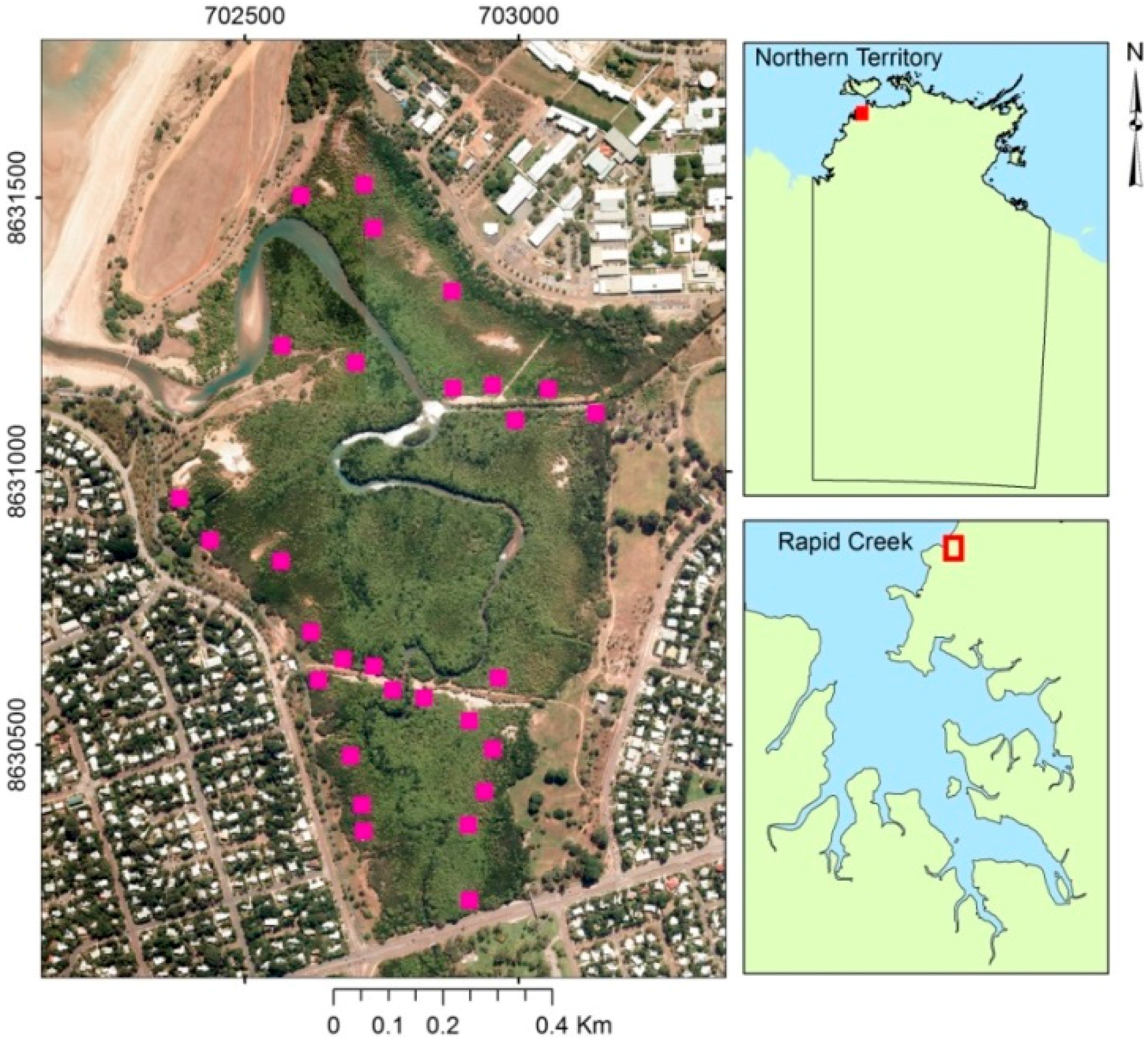
Figure 1. Rapid Creek coastal mangrove forest, Darwin, Northern Territory, Australia. The distribution of field sampling plots (5 m × 5 m) is shown in the map (the sizes of magenta squares are not to the scale). Aerial photographs © Northern Territory Government.
Jimaging 02 00024 g001
Figure 2. Mangrove trees inside the Rapid Creek forest; (AC) small, newly-regenerated mangrove trees; (D,E) large, multi-stemmed mangrove trees; (F,G) densely-clustered areas.
Jimaging 02 00024 g002
Figure 3. Normal score plots of field estimates of (A) leaf area index and (B) log-transformed above ground biomass.
Jimaging 02 00024 g003
Figure 4. Cross-validated predictions for the normalized leaf area index (LAI) and above ground biomass (AGB): (A) predicted versus field measured normalized LAI with 2-m spatial resolution predictor variables; (B) predicted versus field measured normalized LAI with 5-m spatial resolution predictor variables; (C) predicted versus field measured normalized LogAGB with 2-m spatial resolution predictor variables; (D) predicted versus field measured normalized LogAGB with 5-m spatial resolution predictor variables. (RMSEP, root mean square error of prediction).
Jimaging 02 00024 g004
Figure 5. Predicted maps: (A) leaf area index with a 2-m spatial resolution; (B) leaf area index with a 5-m spatial resolution; (C) above ground biomass with a 2-m spatial resolution; and (D) above ground biomass with a 5-m spatial resolution; using the partial least squares regression algorithm. The distribution of field sampling plots is shown in the maps (the sizes of the black squares are not to scale).
Jimaging 02 00024 g005
Table 1. Spectral band information of WorldView-2 images.
BandSpectral Range (nm)Spatial Resolution (m)
Panchromatic447–8080.5
Coastal396–4582
Blue442–515
Green506–586
Yellow584–632
Red624–694
Red-edge699–749
NIR1765–901
NIR2856–1043
Table 2. Predictor variables generated from the WorldView-2 multispectral image for estimating above ground biomass and leaf area index. NIR1, NIR2, red edge, red and green: surface reflectance of Near Infrared 1, Near Infrared 2, red-edge, red and green wavelength regions, respectively.
Vegetation IndexBand RelationshipSource
Normalized Difference Vegetation Index (NDVI) ( NIR 1 red ) / ( NIR 1 + red ) Rouse et al. [24] and Ahamed et al. [10]
Normalized Difference Red Edge index (NDRE) ( NIR 1 Red   Edge ) / ( NIR 1 + Red   Edge ) Ahamed et al. [10] and Barnes et al. [25]
Green Normalized Difference Vegetation Index (GNDVI) ( NIR 1 green ) / ( NIR 1 + green ) Ahamed et al. [10], Li et al. [26] and Gitelson et al. [27]
Green Normalized Difference Vegetation Index 2 (GNDVI2) ( NIR 2 green ) / ( NIR 2 + green ) Mutanga et al. [28]
Normalized Difference Vegetation Index 2 (NDVI2) ( NIR 2 red ) / ( NIR 2 + red ) Mutanga et al. [28]
Normalized Difference Red Edge index 2 (NDRE2) ( NIR 2 Red   Edge ) / ( NIR 2 + Red   Edge ) Mutanga et al. [28]
Renormalized Vegetation Index (RDVI) ( NIR 1 red ) / NIR 1 + red Li et al. [26]
Ratio Vegetation Index (RVI) NIR 1 / red Li et al. [26]
Modified Soil Adjusted Vegetation Index (MSAVI) ( 1 + 0.5 ) ( NIR 1 red ) / ( NIR 1 + red + 0.5 ) Qi et al. [29]
Table 3. Log10-transformed allometric relationships used for different mangrove species. The equations are in the form of l o g 10 ( B i o m a s s ) = B 0 + B 1 * l o g 10 ( D B H ) ; where DBH is the diameter at breast height; B0 and B1 are regression coefficients. These equations are specific to Northern Australia [39,40,41], North-eastern Queensland, Australia [41], and Sri Lanka [20] (biomass in kg and DBH in cm).
Mangrove SpeciesB0B1Study
Avicennia marina−0.5112.113Comley and McGuinness [40]
Bruguiera exaristata−0.6432.141Comley and McGuinness [40]
Ceriops tagal−0.72472.3379Clough and Scott [41]
Lumnitzera racemosa1.7882.529Perera and Amarasinghe [20]
Rhizophora stylosa−0.6962.465Comley and McGuinness [40]
Sonneratia alba−0.6342.248Bai [39]
Excoecaria agallocha var. ovalis−0.6342.248Bai [39]
Table 4. Root mean square errors (RMSEs) and correlation coefficients (r) for above ground biomass and leaf area index maps with respect to the validation samples.
Biophysical VariableRMSECorrelation Coefficient
Spatial resolution2 m5 m2 m5 m
Above ground biomass (AGB)2.2 kg/m22.0 kg/m20.40.8
Leaf area index (LAI)0.750.780.70.8