Automatic Gleason Grading of Prostate Cancer Using Shearlet Transform and Multiple Kernel Learning

Abstract

The Gleason grading system is generally used for histological grading of prostate cancer. In this paper, we first introduce using the Shearlet transform and its coefficients as texture features for automatic Gleason grading. The Shearlet transform is a mathematical tool defined based on affine systems and can analyze signals at various orientations and scales and detect singularities, such as image edges. These properties make the Shearlet transform more suitable for Gleason grading compared to the other transform-based feature extraction methods, such as Fourier transform, wavelet transform, etc. We also extract color channel histograms and morphological features. These features are the essential building blocks of what pathologists consider when they perform Gleason grading. Then, we use the multiple kernel learning (MKL) algorithm for fusing all three different types of extracted features. We use support vector machines (SVM) equipped with MKL for the classification of prostate slides with different Gleason grades. Using the proposed method, we achieved high classification accuracy in a dataset containing 100 prostate cancer sample images of Gleason Grades 2–5.

1. Introduction

1.1. Motivation

Prostate cancer is diagnosed more often than any other cancer in men with the exception of skin cancer [1]. It is estimated that 180,890 new cases of prostate cancer will occur in the U.S. in 2016 [1]. Prostate cancer cells can transfer to other tissues and develop new damaging tumors. Therefore, it is vital to diagnose prostate cancer in the early stages and to provide necessary treatment.

There are several screening methodologies for prostate cancer diagnosis. Histological grading is an essential key in prostate cancer diagnosis and treatment methodology [2]. Cancer aggressiveness is quantified using histological grading of the biopsy specimens of the tissue. The tissue is usually stained by the hematoxylin and eosin (H&E) technique [2].

The Gleason grading system is widely used for prostate grading [3], which classifies the prostate cancer as Grades 1–5, as shown in Figure 1. Higher Gleason grades indicate a higher malignancy level. The Gleason score is calculated using the sum of the two most dominant Gleason grades inside a tissue and ranges from 2 to 10. Patients with a combined score between two and four have a high chance of survival, while patients with a score of 8–10 have a higher mortality rate [2].

To better understand the difference between normal and malignant tissues, we illustrate sample images in Figure 2. Figure 2a shows normal prostate tissue containing gland units enclosed by stroma. Gland units contain epithelial cells around the lumen. When cancer happens, epithelial cells randomly duplicate, disturbing the normal structure of glands, as shown in Figure 2b,c.

Furthermore, the shape of normal and benign cells has a recognizable pattern, while malignant cells are described by irregular morphology in nuclei [6]. Malignant cells have larger nuclei and less cytoplasm than benign cells. Figure 2b,c shows Gleason Grade 2 and 5 malignant tissues, respectively.

Automatic medical image classification is an important field mainly based on image processing methods. Automatic processing of cancer cell images can be less time consuming and more efficient than pathologist examination. Furthermore, computerized analysis is not prone to inter-observer and intra-observer variations resulting from human grading [7]. In this paper, we extract different features, including a new feature based on the Shearlet transform, combine them using multiple kernel learning (MKL) and utilize them for the automatic Gleason grading of prostate.

1.2. Literature Review

Several methods have been proposed for automatic Gleason grading [7,8,9,10,11,12,13,14,15,16]. We categorize those papers based on the features they use and review them in the following. The features are: (1) structural; (2) texture; and (3) color.

Structural techniques are based on cell segmentation and then feature extraction [7,8,9,10,11]. Farjam et al. [7] extracted structural features of the glands and used them in a tree-structured algorithm to classify the images into five Gleason grades of 1–5. First, the gland units were located using texture features. Then, the authors used a multistage classification method based on morphometric and texture features extracted from gland units to classify the image into Grades 1–5. They reported classification accuracies of 95% and 85% on two different datasets using the leave-one-out technique.

Salman et al. [8] extracted joint intensity histograms of hematoxylin and eosin components from the histological images and used k-nearest neighbor supervised classification to delineate the benign and malignant glands. They compared their results with the histogram of oriented gradients and manual annotation by a pathologist and showed that their method outperformed the other methods.

Gertych et al. [9] extracted intensity histograms and joint distributions of the local binary patterns and local variance features and used a machine learning approach containing a support vector machine followed by a random forest classifier to classify prostate tissue into stroma, benign, and prostate cancer regions.

Khurd et al. [10] used random forests to cluster the filter responses from a rotationally-invariant filter bank at each pixel of the histological image into textons. Then, they used the spatial pyramid match kernel along with an SVM classifier to classify different Gleason grade images.

A microscopic image segmentation method was proposed in [11]. The authors transformed the images to the HSV domain and used mean shift clustering for segmentation. They extracted texture features from the cells and used an SVM classier to classify lymphocytes.

Some other techniques are based on texture features or a combination of texture, color and morphological features [12,13,14,15,16]. Jafari and Soltanian-Zadeh [5] used multiwavelets for the task of automatic Gleason grading of prostate. The authors compared the results from features based on multiwavelets with co-occurrence matrices and wavelet packets. They used a k-nearest neighbor classifier to classify images. They assigned weights on features and optimized those weights using simulated annealing. They report an accuracy of 97% on a set of 100 images using the leave-one-out technique.

Tabesh et al. [12] proposed a multi-feature system for the task of cancer diagnosis and Gleason grading. The authors combined color, texture and morphometric features for classification. They used 367 images for cancer detection and reported 96% accuracy. They also used 268 images for Gleason grading and reported 81% classification accuracy.

In a recent study, we used Shearlet coefficients for the automatic diagnosis of breast cancer [13]. We extracted features from multi-decomposition levels of Shearlet filters and used the histogram of Shearlet coefficients for the task of classification of benign and malignant breast slides using SVM. We applied our proposed method on a publicly-available dataset [14] containing 58 slides of breast tissue and achieved 75% classification accuracy. We also used the Shearlet transform for prostate cancer detection of histological images [15] and MR images [16], and we achieved 100% and 97% classification accuracy, respectively.

Compared to our previous work [13,14,15,16], we have two novelties in this paper. First, despite our previous studies where we used the histogram of Shearlet coefficients, here, we extract more statistics from Shearlet coefficients using a co-occurrence matrix. This provides more information on the texture of the cancerous tissues, which in turn results in higher classification rates for the task of Gleason grading as presented in our Experimental Results section. Second, we utilize other types of features (color and morphological) and combine them using MKL, which makes our proposed method in this paper more comprehensive.

1.3. Proposed System Overview

Image classification problems rely on feature descriptors that point out the differences and similarities of texture while robust in the presence of noise [17]. However, different applications need different feature descriptors. Therefore, there is an extensive amount of research carried out on finding the best feature extraction methods. In this paper, we propose to use three different types of features and fuse them using MKL [18].

Our main contribution in this paper is two-fold. First, we propose using the Shearlet transform and its coefficients as texture features for automatic Gleason grading of prostate cancer. Traditional frequency-based methods cannot detect directional features [19]. On the other hand, the Shearlet transform [20] can detect features in different scales and orientations and provides efficient mathematical methods to find 2D singularities, such as image edges [21,22,23]. The Gleason grading images are typically governed by curvilinear features, which justifies the choice of the Shearlet transform as our main texture features.

Second, we utilize the multiple kernel learning algorithm [18] for fusing three different types of features used in our proposed approach. In multiple kernel learning, a kernel model is constructed using a linear combination of some fixed kernels. The advantage of using MKL is in the nature of the classification problem we are trying to solve. Since we have different types of features extracted from images, it is possible to define a kernel for each of these feature types and to optimize their linear combination. This will eliminate the need for feature selection.

After we extracted the features, we use support vector machines (SVM) equipped with MKL for the classification of prostate slides with different Gleason grades. Then, we compare our results with the state of the art. The overall system is depicted in Figure 3.

The remainder of this paper is organized as follows. In the next section, three different types of image features are presented. In Section 3, feature fusion using the MKL algorithm and SVM-based classification is reported. In Section 4, we report the classification results. Finally, the conclusions are presented in Section 5.

2. Feature Analysis of Microscopic Images

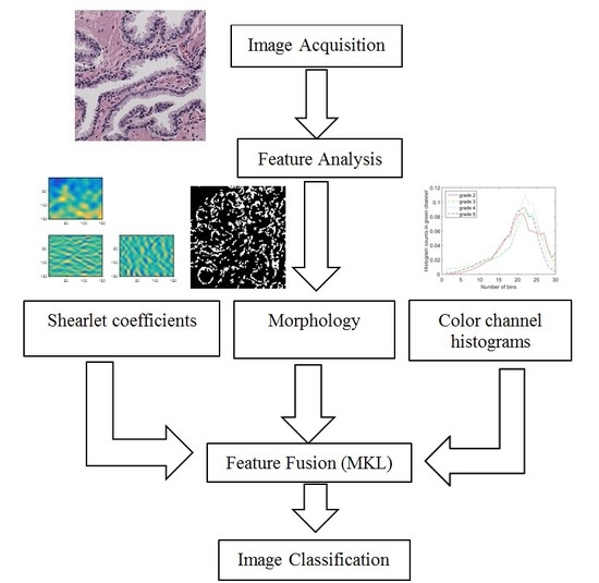
As described in the previous section, Gleason grading is based on different properties of the tissue image. Therefore, we need a robust feature extraction method that considers all of the possible changes in the tissue due to cancer. In this section, we present features representing the color, texture and morphological properties of the cancerous tissues. These features are the essential building blocks of what pathologists consider when they perform Gleason grading. Some of the parameters in the following section, such as the number of histogram bins in color channel histograms, were selected based on our preliminary results.

2.1. Texture Features

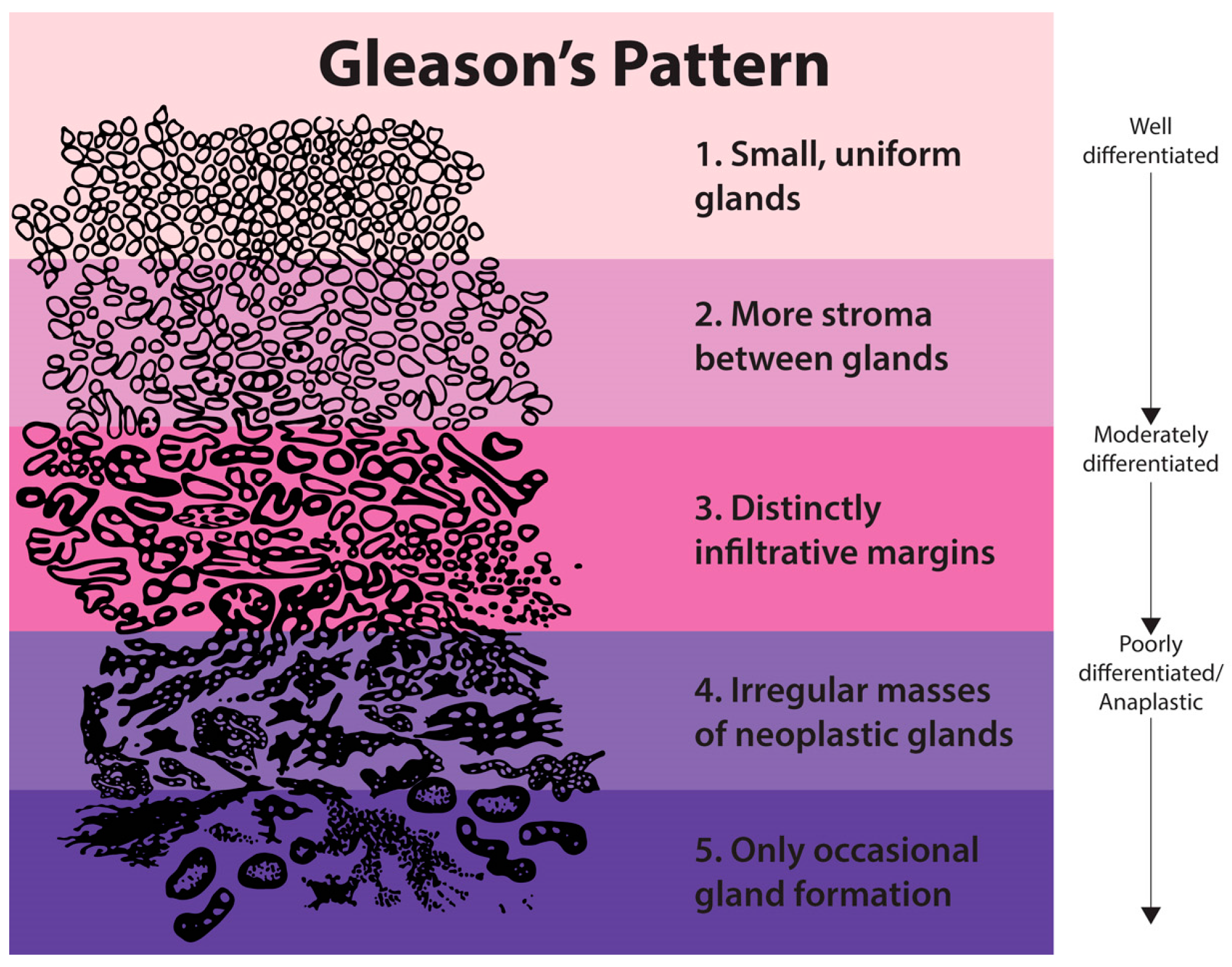
Gleason grading is mainly based on texture features and the characteristics of the cancerous tissues. Taking another look at Figure 1 highlights the changes in texture due to malignancy by observing that the texture becomes more detailed as the epithelial cell nuclei grow in a random manner and spread across the tissue. Therefore, we need to develop the most novel, accurate and robust texture analysis tool. For this purpose, we propose a novel feature representation method using the statistics extracted from discrete Shearlet coefficients.

2.1.1. Shearlet Transform

We utilize the Shearlet transform [19,20] as our main texture detection method. The Shearlet transform is a new method that is efficiently developed to detect 1D and 2D directional features in images.

The curvelet transform was the pioneer of the new set of transforms [24]. Curvelets are defined by three parameters: scale, location and rotation. However, the curvelet is sensitive to rotation, and a rotation breaks its structures. Furthermore, curvelets are not defined in the discrete domain; therefore, it made it impractical for real-life applications. Therefore, we need a directional representation system that can detect anisotropic features in the discrete domain. To overcome this limitation, the Shearlet transform was developed based on the theory of affine systems. The Shearlet transform uses shearing instead of rotation, which in turn allows for discretization. The continuous Shearlet transform [19] is defined as the mapping for $f ϵ L^2(R^2)$:

$$S{H}_{\Psi }f\left(a,s,t\right)= <f,{\Psi }_{a,s, t}>$$

(1)

Then, the Shearlets are given by:

$${\Psi }_{a,s,t}\left(x\right)={\left|det{M}_{a,s}\right|}^{-\frac{1}{2}}\Psi \left({M_{a,s}}^{-1}x-t\right)$$

(2)

where $M_{a,s}=\left(\begin{array}{cc}a& \sqrt{a}s\\ 0& \sqrt{a}\end{array}\right)$ for $a>0,s ϵ R,t ϵ R^2$. We can observe that $M_{a,s}=B_s{A}_a$, where $A_a=\left(\begin{array}{cc}a& 0\\ 0& \sqrt{a}\end{array}\right)$ and $B_s=\left(\begin{array}{cc}1& s\\ 0& 1\end{array}\right)$. Hence, $M_{a,s}$ consists of an anisotropic dilation produced by the matrix $A_a$ and a shearing produced by the matrix $B_s$. As a result, the Shearlets are well-localized waveforms.

By sampling the continuous Shearlet transform in the discrete domain, we can acquire the discrete Shearlet transform [20]. Choosing $a=2^{-j}$ and $s=-l$ with $j,l ϵ Z$, one can acquire the collection of matrices $M_{2^{-j},-l}$. By observing that ${M_{2^{-j},-l}}^{-1}=M_{2^j,l}=\left(\begin{array}{cc}{2}^j& l{2}^{j/2}\\ 0& 2^{j/2}\end{array}\right)={B_0}^l{A_0}^j,$ where $A_0=\left(\begin{array}{cc}2& 0\\ 0& \sqrt{2}\end{array}\right)$ and $B_0=\left(\begin{array}{cc}1& l\\ 0& 1\end{array}\right)$, the discrete system of Shearlets can be represented as:

$${\Psi }_{j,l,k}={\left|det{A}_0\right|}^{\frac{j}{2}}\Psi \left({B_0}^l{A_0}^{j}x-k\right)$$

(3)

where $j,l ϵ Z, k ϵ Z^2$. The discrete Shearlets can deal with multidimensional functions. Due to the simplicity of the mathematical structure of Shearlets, their extensions to higher dimensions are very natural [25].

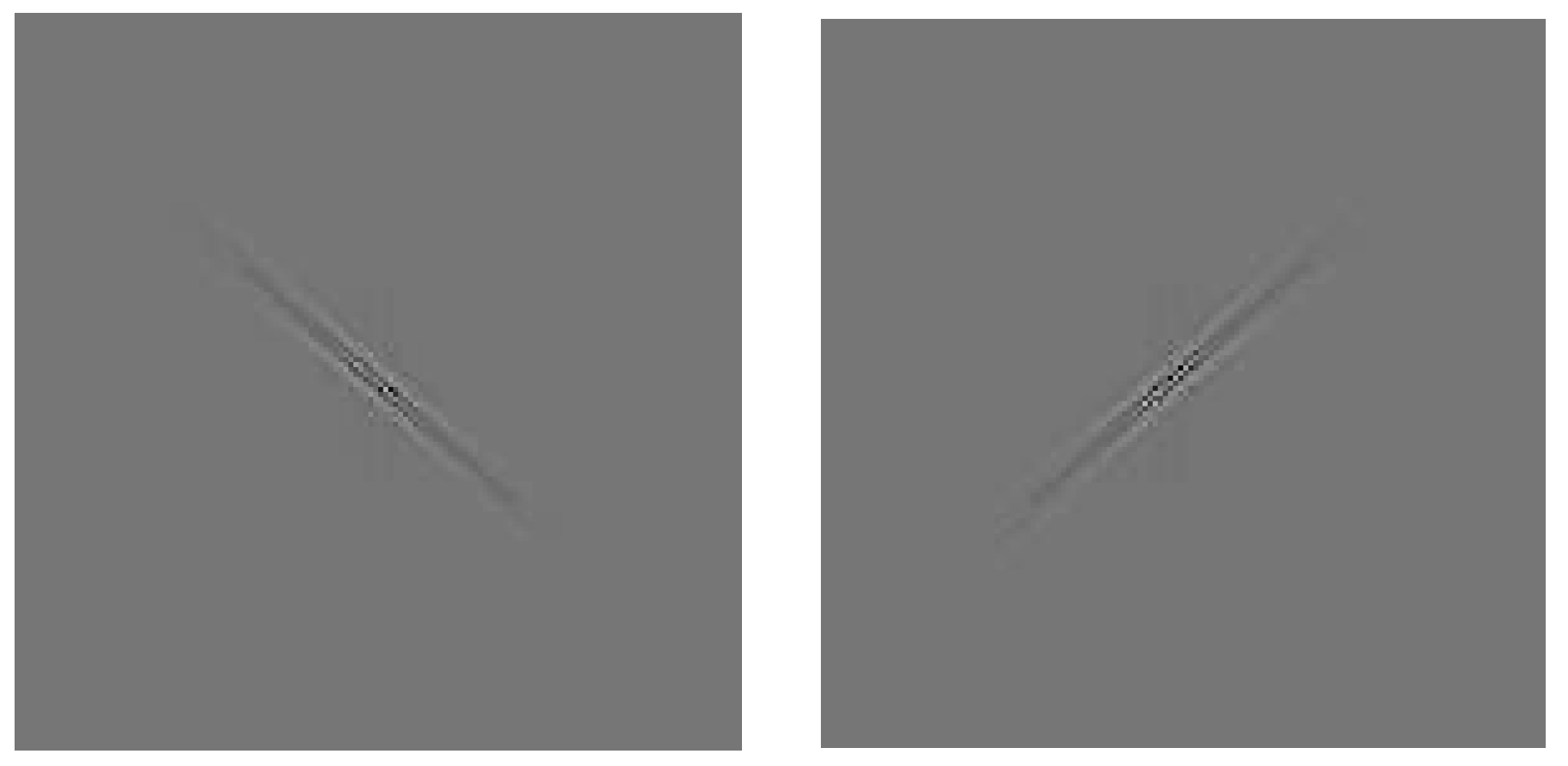
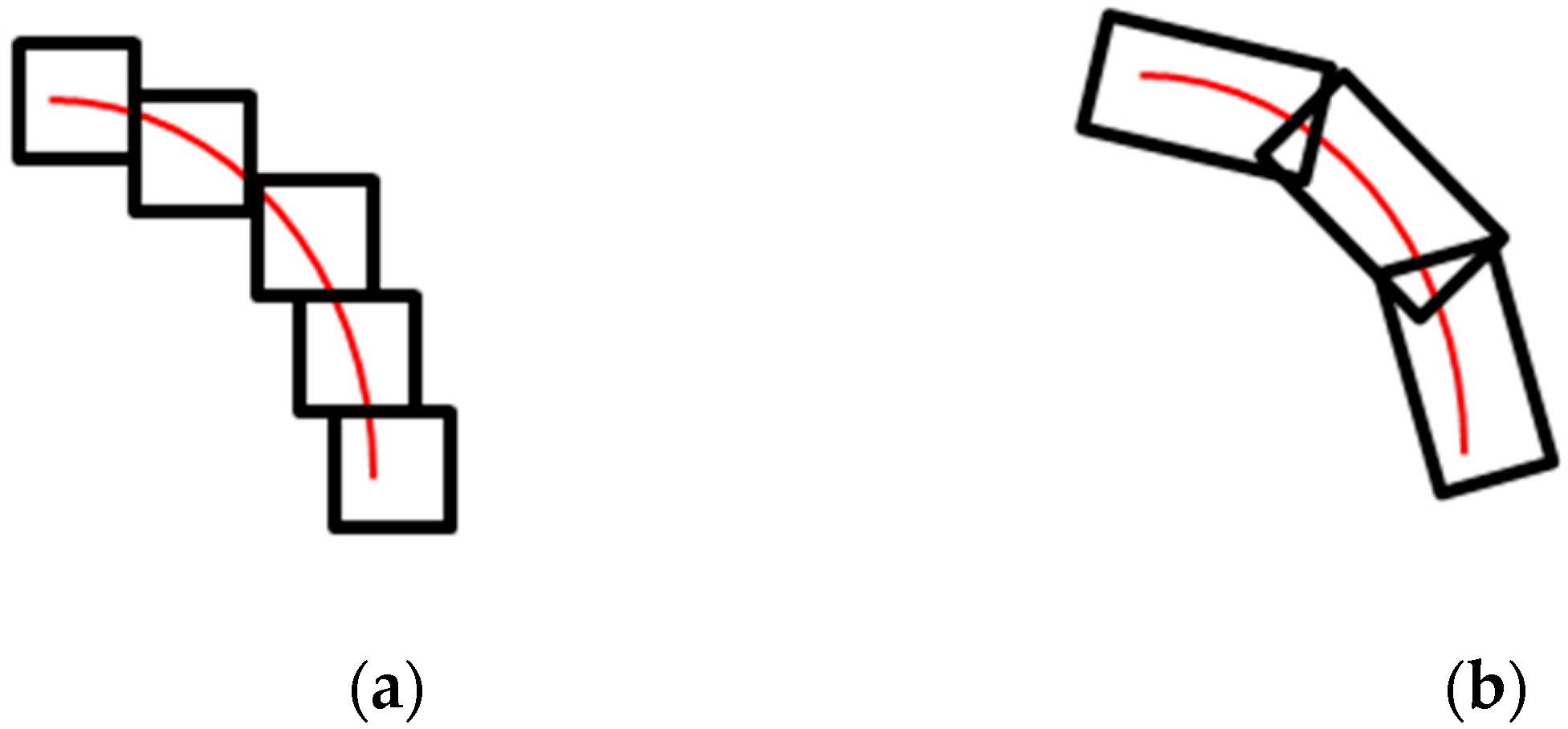
The discretized Shearlet system often forms a frame, which allows for a stable representation of images. This justifies this way of discretization. Furthermore, Shearlets are scaled based on parabolic scaling, which makes them appear as elongated objects in the spatial domain, as shown in Figure 4.

To better understand the advantage of the Shearlet transform over wavelet transforms, we further discuss their scaling properties. Wavelets are based on isotropic scaling, which makes them isotropic transforms and, therefore, not suitable for detecting non-isotropic objects (e.g., edges, corners, etc.) [26,27,28]. On the other hand, since the Shearlet transform defines the scaling function using parabolic scaling, it can detect curvilinear structures, as shown in Figure 5. We refer our readers to [25] for more details on the Shearlet transform and its properties.

2.1.2. Features Extracted from the Shearlet Transform

After we calculated discrete Shearlet coefficients of the images in our dataset, we find the co-occurrence matrix of the Shearlet coefficients. This will give us the information we need about the texture of the images since Shearlet coefficients are good representatives of the heterogeneity of images. Features extracted from the co-occurrence matrix have been shown to be useful in image analysis [29]. A co-occurrence matrix of an image represents the probability distribution of the occurrence of two pixels separated by an offset. The offset is a vector with rows and columns that represent the number of rows/columns between the pixel of interest and its neighbor. To find the co-occurrence matrix, we follow the procedure described in [29]. 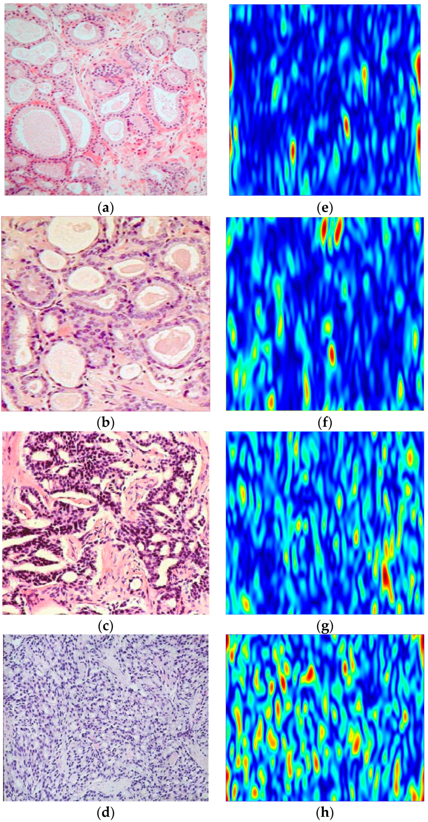After calculating the co-occurrence matrix for Shearlet coefficients of each image, we extract 20 different statistical features from the co-occurrence matrix, as explained in [29,30,31,32]. These features are energy, correlation, entropy, autocorrelation, contrast, cluster prominence, cluster shade, dissimilarity, homogeneity, maximum probability, sum of squared variance, sum of average, sum of variance, sum of entropy, difference of variance, difference of entropy, information measure of correlation, inverse difference and inverse difference momentum. Therefore, we extract a feature vector of size 1 × 20 for each image. To further illustrate the capabilities of the Shearlet transform to highlight the singularities in the images, we show the third decomposition level Shearlet coefficients of the sample Gleason Grades 2, 3, 4 and 5 images in Figure 6. As the Gleason grade increases from Grade 2 (Figure 6a) to Grade 5 (Figure 6d), the Shearlet coefficients highlight the structure of the cell and the random scattering of the epithelial cells more vividly.

2.2. Color Features

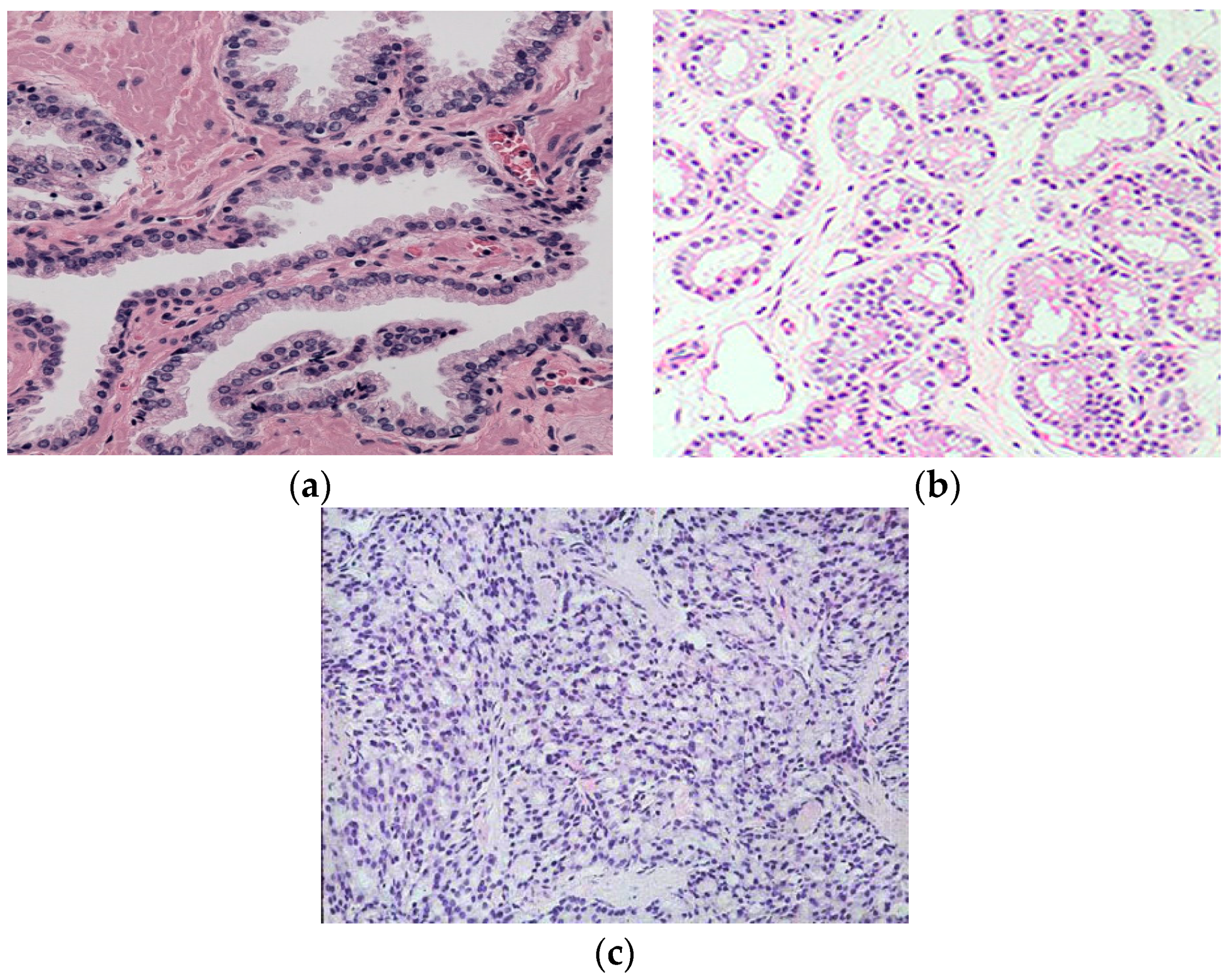
By looking closely at different Gleason grade images, we can find visible color changes as images transform from Gleason Grade 2 to Grade 5, as shown in Figure 2. The reason behind this is that as the Gleason grade increases, the blue-stained epithelial cell nuclei invade the pink-stained stroma and white-colored lumen regions. Therefore, we can use color channel histograms to represent the change in color due to the changes in epithelial cell nuclei area.

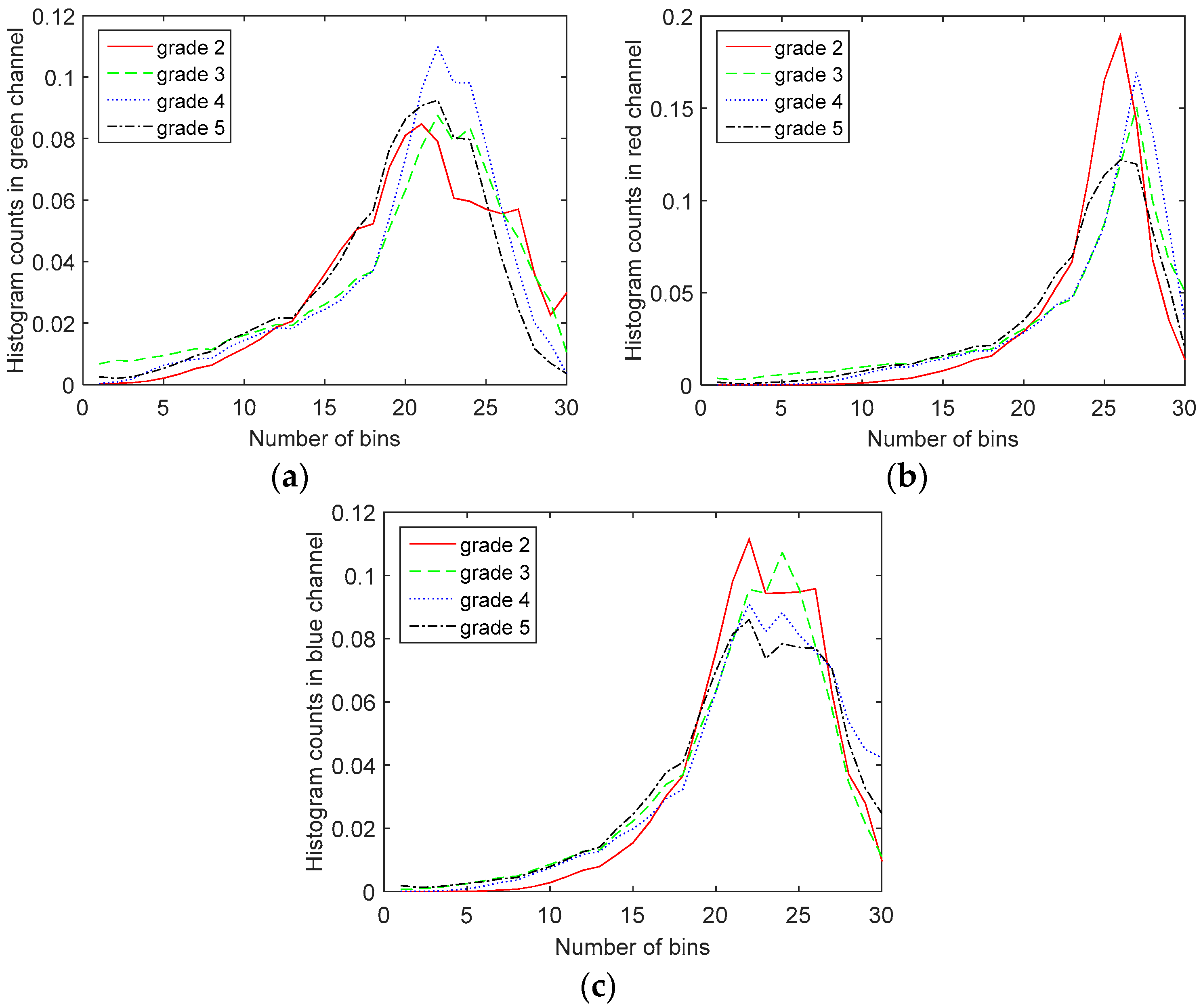
To further investigate the differences in the color channel histograms of different Gleason grade images, we have shown the red, green and blue color channel histograms of the Gleason Grades 2–5 images of prostate in Figure 6. It can be observed from the histogram of the green channel that as the Gleason grade increases, the histogram moves towards lower green channel intensity values (lower number of counts in the green channel). This is in accordance with the results from [12]. It should be mentioned that the values on the graphs are the average values of histogram counts over the whole dataset, since we observed large within-class variations for histograms. As explained in [12], these variations are due to the heterogeneous nature of prostate tissue and the fact that the images are taken from different parts of the prostate.

However, we cannot derive the same conclusion from red or blue channel histograms, as shown in Figure 7. Therefore, we include more information in our features using different color space histograms. For that purpose, we have also calculated the histograms of the YCbCr, HSV, CIELAB and CIELUV color spaces, as well [33]. By converting from the RGB to the YCbCr color space, the main colors related to red, green and blue are processed into less redundant and more meaningful information. Human perception of color can be best exploited by the HSV (hue, saturation, value) color space, which makes it more favorable in our case of the H&E images of prostate tissue. The CIELAB color space is designed to approximate human vision and matches human perception of lightness. The CIELUV is also another color space that fits human perception of colors better than the original RGB color space.

Overall, we have five color spaces; each has three components. For each image, we find the histogram of each component of each color space using 30 bins, which returned the best preliminary evaluation results. Then, we normalize each histogram by dividing it by the number of pixels in the image, so that it is independent of the image size. Therefore, for each image, we extract 15 color channel histograms each of a size of 30 × 1. Therefore, we have a feature vector of a size of 450 × 1.

2.3. Morphological Features

Morphological changes of the tissue due to malignancy also play an important role in Gleason grading. As we described in Section 1, cell nuclei of malignant tissues contain the most important information of malignancy. The malignant cell nuclei are larger than benign cell nuclei and have different sizes and forms. This motivated us to base our morphological feature extraction algorithm on cell nuclei detection. To achieve this, we propose using the mean shift clustering algorithm [34] for the task of color approximation and then thresholding in HSV color space to separate cell nuclei from other parts of the tissue, similar to [11]. The mean shift algorithm uses a window around each data point and calculates the mean. Then, it shifts the window to the mean and repeats until convergence. Based on this algorithm, the window moves to a congested area of the data, helping us find the more important parts of the data.

The application of the mean shift algorithm in image segmentation has already been investigated in [34]. However, we discovered for cell nuclei segmentation in H&E images that we need to take further steps. Therefore, after initial segmentation using the mean shift algorithm, which reduced the number of distinct colors, we convert the segmented image to the HSV domain and apply a threshold in the HSV domain to separate cell nuclei from other parts of the tissue, similar to [11]. As we described earlier, human perception of color can be best exploited by the HSV color space, which makes it more favorable in our case of H&E images of prostate tissue. To apply the threshold to separate blue hue (cell nuclei) from pink hue (other parts of tissue), we found a fixed empirical threshold and applied it based on the following algorithm:

$$M\left(i,j\right)=\{\begin{array}{c}1, if 0.70\le hue\left( i , j \right)\le 0.88\\ 0, otherwise\end{array}$$

(4)

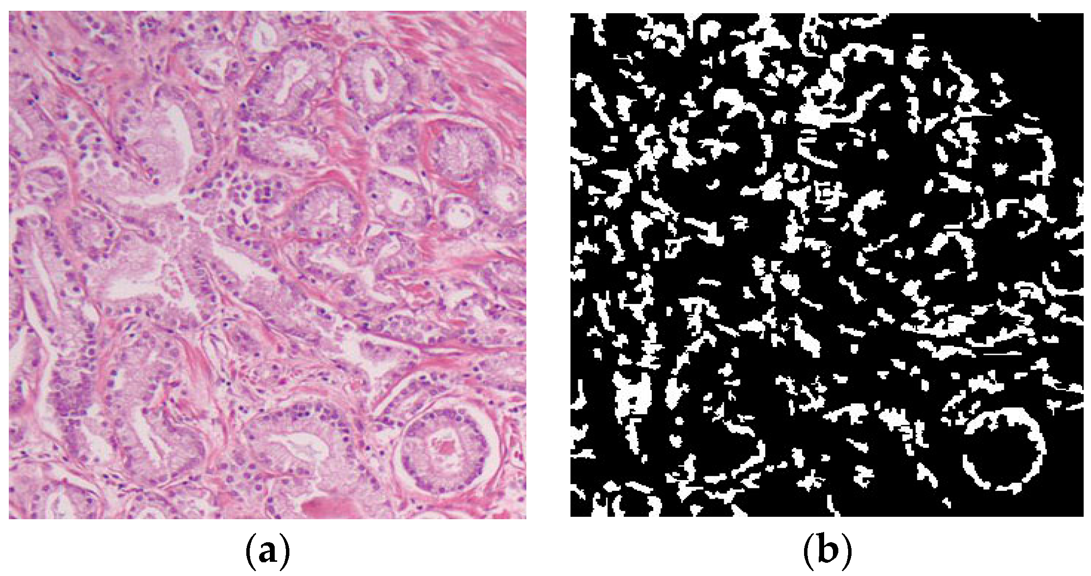
where $M$is the mask created after thresholding the image, $i$ and $j$ are the indices of image pixels and $hue$ is the hue value of the output of the mean shift after converting to the HSV domain. The output of the cell nuclei segmentation algorithm along with the input image are shown in Figure 8.

After we segmented the cell nuclei, we calculate the cell nuclei area by simply calculating the number of white pixels in the resulting mask and use that as a morphological feature for automatic Gleason grading.

3. Feature Fusion Using Multiple Kernel Learning

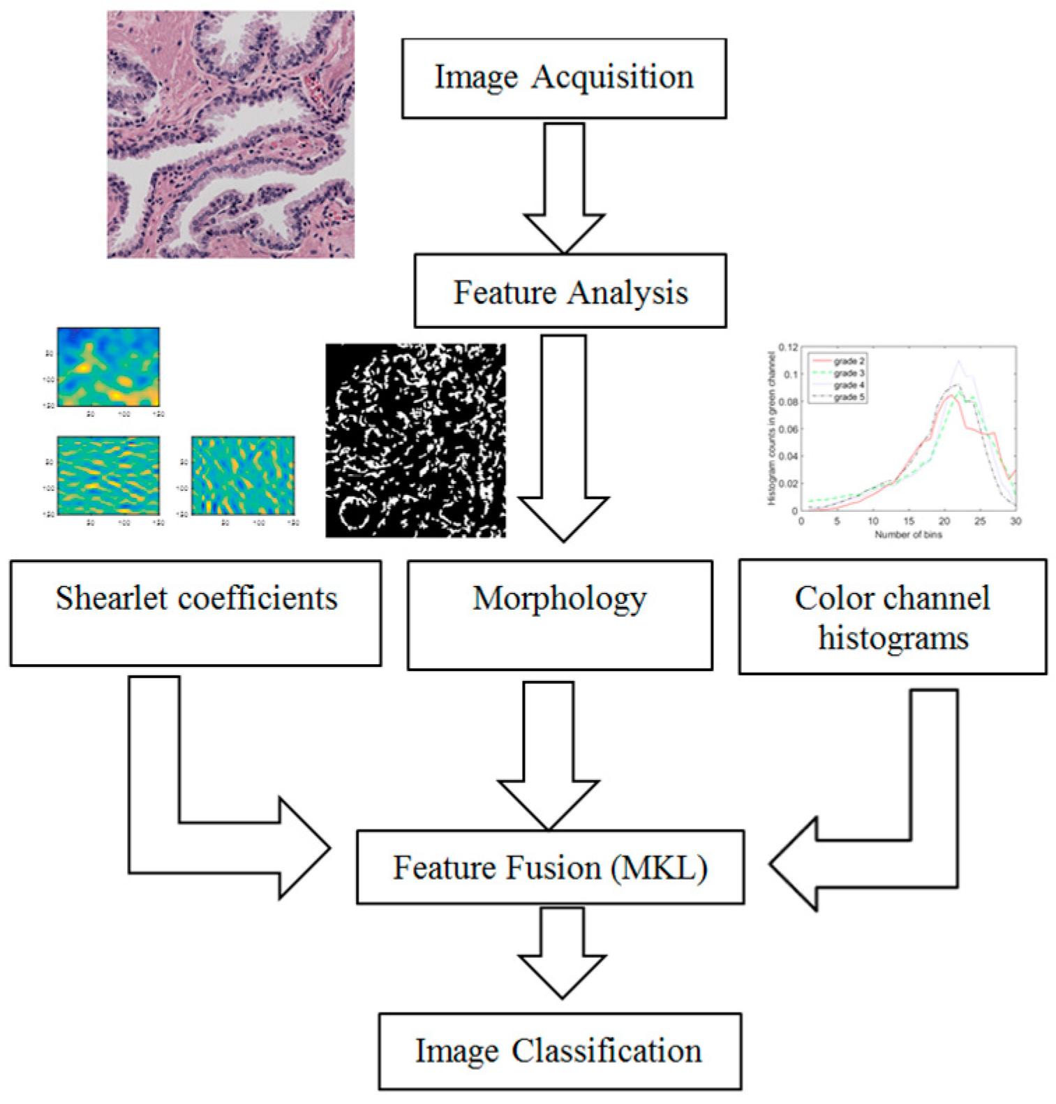
In the previous section, we described extracting three features: color channel histograms, statistics from discrete Shearlet coefficients and morphological features. Now, we combine these features in an intelligent manner that finds the best way to represent and use them for image classification. We use a state of the art feature fusion/classification technique called SimpleMKL [18], which is based on multiple kernel learning algorithm. MKL is suitable for fusing heterogeneous features [35]. There are two reasons to choose MKL for feature fusion: (1) MKL is designed for simultaneous learning and classification and, therefore, eliminates our need to design a feature selection step; (2) it matches with our problem, since we have different representations of data. Therefore, merging kernels is a reliable way to use different sources of information [35].

To describe the feature fusion using MKL, first, we start with the SVM algorithm, which is the most commonly-used base learner for MKL due to its empirical success, ease of applicability as a building block in two-step methods and also ease of transformation to other optimization problems as a one-step training method using the simultaneous approach [35]. Then, we explain the general MKL problem and the reasoning behind it. Finally, we describe the SimpleMKL algorithm and its application for multiclass SVM.

SVM is a non-probabilistic linear classifier for binary classification problems. Given a sample of N training instances ${\left\{\left(x_i,y_i\right)\right\}}_{i=1}^N$ where $x_i$ is the $D$-dimensional input vector and $y_i\in \left\{-1,+1\right\}$ is its class label, SVM finds the linear discriminant with the maximum margin in the feature space using the mapping function Φ: $R^D\to R^S$. The resulting discriminant function is:

$$f\left(x\right)=W^T\mathsf{\Phi }\left(x\right)+b$$

(5)

where $W$ is the normal vector to the hyperplane. The classifier can be trained by finding two hyperplanes in a way that they separate the data, which leads to the following quadratic programming optimization problem:

$$\text{minimize} \frac{1}{2}{||w||}_2^2+C{\sum }_{i=1}^N{\xi }_i$$

$$\text{with respect to} W\in R^S,\xi \in R_{+}^N, b\in R$$

(6)

$$\text{subject to} y_i\left(W^T\mathsf{\Phi }\left(x_i\right)+b\right)\ge 1-{\xi }_i \forall i$$

where $W$ is the weight vector, $C$is a positive trade-off parameter between model simplicity and classification error, $\xi$ is the vector of slack variables, which measure the degree of misclassification of the data, and $b$ is the bias term of the separating hyperplane. We can find the following dual formulation using the Lagrangian dual function:

$$\text{maximize} {\sum }_{i=1}^N{\alpha }_i-\frac{1}{2}{\sum }_{i=1}^N{\sum }_{j=1}^N{\alpha }_i{\alpha }_j{y}_i{y}_{j}K(x_i,x_j)$$

$$\text{with respect to} \alpha \in R_{+}^N$$

(7)

$$\text{subject to} {\sum }_{i=1}^N{\alpha }_i{y}_i=0, 0\le {\alpha }_i\le C \forall i$$

where $K\left(x_i,x_j\right)=\mathsf{\Phi }{\left(x_i\right)}^{\mathrm{T}}\mathsf{\Phi }\left(x_j\right):R^D\times R^D\to R$ is called the kernel function and $\alpha$ is the vector of dual variables corresponding to each separation constraint. The key advantage of a linear penalty function is that the slack variables vanish from the dual problem, with the constant $C$ appearing only as an additional constraint on the Lagrange multipliers.

Solving the above optimization problem, we get $W={\sum }_{i=1}^N{\alpha }_i{y}_i\mathsf{\Phi }\left(x_i\right)$, and the discriminant function can be rewritten as:

$$f\left(x\right)={\displaystyle \sum }_{i=1}^N{\alpha }_i{y}_{i}K\left(x_i,x\right)+b$$

(8)

Some of the most favorable kernel functions in the literature are linear, polynomial and Gaussian, which are presented in the following:

$$K_{LIN}\left(x_i,x_j\right)=x_i.x_j$$

$$K_{POL}\left(x_i,x_j\right)={\left(x_i.x_j+1\right)}^q, q\in N$$

(9)

$$K_{GAU}\left(x_i,x_j\right)=e^{-{||x_i-x_j||}_2^2/2S^2}, S\in R^{++}$$

The above kernel functions are each favorable for a specific type of data. Therefore, selecting the kernel function $K\left(·,·\right)$ and its parameters (e.g., $q$or $s$) is an important issue in training. Recently, MKL methods have been proposed, where we combine multiple kernels instead of selecting one specific kernel function and its corresponding parameters. There are two advantages with MKL: (a) different kernels correspond to different notions of similarity, and instead of trying to find which works best, a learning method does the picking for us, or we may use a combination of them; (b) different kernels may be using inputs coming from different representations possibly from different sources or modalities. Since these are different representations, they have different measures of similarity corresponding to different kernels. In such a case, combining kernels is one possible way to combine multiple information sources [36]. We can find the combination function using the following formula:

$$K_d\left(x_i,x_j\right)=f_d\left({\left\{K_m\left({x_i}^m,{x_j}^m\right)\right\}}_{m=1}^p|d\right)$$

(10)

where $f_d:R^p\to R$ is the combination function, ${\left\{K_m:R^{D_m}\times R^{D_m}\to R\right\}}_{m=1}^p$ are the kernel functions that take $P$ feature representations of data instances: $x_i={\left\{{x_j}^m\right\}}_{m=1}^p$ where ${x_j}^m\in R^{D_m}$ and $D_m$ is the dimensionality of the corresponding feature representation. In the above implementation, different parameters are used to combine a set of predefined kernels.

There is a significant amount of work in the literature for combining multiple kernels. In this paper, we propose using a well-known multiple kernel learning algorithm called SimpleMKL [18]. Rakotomamonjy et al. [18] proposed a different primal problem for MKL and used a gradient descent method to solve this optimization problem. They addressed the MKL problem through a weighted two-norm regularization formulation with an additional constraint on the weights that encourages sparse kernel combinations. Then, they solved a standard SVM optimization problem, where the kernel is defined as a linear combination of multiple kernels. Their proposed primal formulation is:

$$\text{minimize} \frac{1}{2}{\sum }_{m=1}^p\frac{1}{d_m}{||w_m||}_2^2+C{\sum }_{i=1}^N{\xi }_i$$

$$\text{with respect to} w_m\in R^{S_m},\xi \in R_{+}^N, b\in R,d\in R_{+}^p$$

(11)

$$\text{subject to} y_i({\sum }_{m=1}^p{W_m}^T{\mathsf{\Phi }}_{\mathrm{m}}\left({x_i}^m\right)+b)\ge 1-{\xi }_i \forall i, {\sum }_{m=1}^p{d}_m=1$$

Then, they define the optimal SVM objective function value given $d$ as $J\left(d\right)$:

$$\text{minimize} J\left(d\right)=\frac{1}{2}{\sum }_{m=1}^p\frac{1}{d_m}{||w_m||}_2^2+C{\sum }_{i=1}^N{\xi }_i$$

$$\text{with respect to} w_m\in R^{S_m}, \xi \in R_{+}^N, b\in R$$

(12)

$$\text{subject to} y_i({\sum }_{m=1}^p{W_m}^T{\mathsf{\Phi }}_{\mathrm{m}}\left({x_i}^m\right)+b)\ge 1-{\xi }_i \forall i$$

The above formulation can be seen as the following constrained optimization problem:

$$\text{minimize} J\left(d\right)$$

$$\text{with respect to} d\in R_{+}^p$$

(13)

$$\text{subject to} {\sum }_{m=1}^p{d}_m=1$$

They proposed SimpleMKL to solve this optimization problem, which consists of two main steps: (a) solving a canonical SVM optimization problem with given $d$; and (b) a reduced gradient algorithm for updating $d$ using the following gradient calculated from the dual formulation assuming that $\alpha$ found in the first step is fixed:

$$\frac{\partial J\left(d\right)}{\partial d_m} =\frac{\partial }{\partial d_m}({\displaystyle \sum }_{i=1}^N{\alpha }_i-\frac{1}{2}{\displaystyle \sum }_{i=1}^N{\displaystyle \sum }_{j=1}^N{\alpha }_i{\alpha }_j{y}_i{y}_j{\displaystyle \sum }_{m=1}^p{d}_m{K}_m\left(x_i,x_j\right)) =-\frac{1}{2}{\displaystyle \sum }_{i=1}^N{\displaystyle \sum }_{j=1}^N{\alpha }_i{\alpha }_j{y}_i{y}_j{K}_m\left(x_i,x_j\right) \forall m$$

(14)

The above formulation is for binary classification tasks. However, since in this paper, we are dealing with multiclass problem, we will use their multiclass multiple kernel learning approach. Suppose we have a multiclass problem with $P$ classes. For a one-against-all multiclass SVM, we need to train $P$ binary SVM classifiers, where the $P$-th classifier is trained by considering all examples of class $P$ as positive examples, while all other examples are considered negative. To extend their approach to multiclass multiple kernel learning, they define a new objective function:

$$O\left(d\right)={\displaystyle \sum }_{p\in P}{O}_p\left(d\right)$$

(15)

where $p$ is the set of all pairs and $O_p\left(d\right)$ is the binary SVM objective value for pair $p$. After defining the new objective function as above, we can follow the rest of the SimpleMKL algorithm. We can find the gradient of $O\left(d\right)$ using:

$$\frac{\partial O\left(d\right)}{\partial d_m}=-\frac{1}{2}{\displaystyle \sum }_{p\in P}{\displaystyle \sum }_{i=1}^N{\displaystyle \sum }_{j=1}^N{\alpha }_{i,p}{\alpha }_{j,p}{y}_i{y}_j{K}_m\left(x_i,x_j\right) \forall m$$

(16)

where ${\alpha }_{j,p}$ is the Lagrange multiplier of the j-th example involved in the P-th decision function. The approach described above tries to find the combination of kernels that jointly optimizes all binary classification problems. We will use this approach in our experiments for the task of Gleason grading.

4. Experimental Results

We used the tissue sample images utilized in the experiments presented in [5]. There were 100 H&E microscopic prostate tissue sample images in the dataset. The acquired images were of Gleason Grades 2–5 graded by an expert, so we had ground truth labels. When extracting the features, we divided the features by the image size to normalize them and have a fair comparison between images with different sizes. For Shearlet coefficient features, we transformed the color images to grayscale to simplify the calculations, since the color of the image did not have any information in this set of features. However, for color channel histogram features and also morphological features, we used the original color images, since these features require color information for further processing.

For sampling images for training and testing of our classification algorithms throughout all experiments, we divided our dataset into training, validation and test sets. Out of 100 images in our dataset, we randomly chose 60 images for training, 10 images for validation (setting the SVM hyperparameters) and the remaining 30 images for testing. We ran this process 50 times and reported the average values of the performance measures for classification. These measures were sensitivity, specificity, F-1 score and accuracy. We found the sensitivity, specificity and F-1 score for each class separately and then reported the average values of them over all four classes. For each image after extracting features, we chose the first few eigenvectors that captured at least 90% of the total variance using the principle component analysis (PCA) method. We used the one-against-all multiclass classification technique. For each type of feature, Gaussian and polynomial kernel functions with different parameters were linearly combined to classify the different Gleason grade images using a multiclass-SVM classifier as follows:

$$K_{POL}\left(x_i,x_j\right)={\left(x_i.x_j+1\right)}^q, q\in N$$

(17)

$$K_{GAU}\left(x_i,x_j\right)=e^{{-||x_i-x_j||}_2^2/2S^2}, S\in R^{++}$$

where $q$ is the degree of the polynomial function and $S$ is the sigma value of the Gaussian function. In our experiments for the Gaussian function, we set $S$ having the values of [0.5, 1, 2, 5, 7, 10, 15, 20, 100, 1000], and for the polynomial kernel, we set $q\in \left[1, 2, 3\right]$. Therefore, given the i-th and j-th samples, the fusion of extracted color features ($\left\{x_i,x_j\right\}$), Shearlet features ($\left\{y_i,y_j\right\}$) and morphological features ($\left\{z_i,z_j\right\}$) is managed as follows:

$$K_{i,j}={\displaystyle \sum }_{m=1}^{13}\left[d_m{k}_m\left(x_i,x_j\right)+d_{m+13}{k}_{m+13}\left(y_i,y_j\right)+ d_{m+26}{k}_{m+26}\left(z_i,z_j\right)\right]$$

(18)

where $k_m\left(.,.\right)$ is one of the 13 kernel functions as described above and $d={\left(d_1,d_2,\dots ,d_{39}\right)}^T \left({||d||}_p=1, p\ge 1\right)$ is the kernel weight vector.

We also included the baseline methods “average” and “product” kernels as suggested by [36]. We followed the following formulas to find the average and product kernels:

$$K_{{Average}_{i,j}}=\frac{1}{13}{\displaystyle \sum }_{m=1}^{13}{k}_m\left(x_i,x_j\right)$$

(19)

$$K_{{Product}_{i,j}}={({\displaystyle \prod }_{m=1}^{13}{k}_m\left(x_i,x_j\right))}^{\frac{1}{13}}$$

4.1. Classification Results Using Color Features

For color channel histograms, we followed the procedure explained in Section 2. Overall, we had five color spaces; each had three components, resulting in 15 color channels in total. For each image, we found the histogram of each component of each color space using 30 bins, which returned the best preliminary evaluation results. Then, we normalized each histogram by dividing it by the number of pixels in the image, so that it was independent of image size. Therefore, for each image, we extracted 15 color channel histograms each of a size of 30 × 1. The combined feature set was of a size of 450 × 1.

The classification results using the single-kernel SVM are presented in

Table 1. Average classification results for color channel histograms.

Color Channel	Sensitivity %	Specificity %	F-1 Score %	Accuracy %
Red	73	90	70	74 ± 9
Green	84	94	82	82 ± 9
Blue	78	92	74	75 ± 9
Y	80	93	78	77 ± 10
Cb	73	91	71	74 ± 10
Cr	75	89	72	75 ± 8
Hue	82	94	80	80 ± 9
Saturation	78	92	75	78 ± 8
Value	74	91	72	72 ± 9
L	76	93	74	77 ± 8
A	72	91	69	74 ± 9
B	76	92	74	75 ± 9
L′	73	90	75	76 ± 9
U	74	91	72	75 ± 8
V	72	90	70	74 ± 9
Combined	90	96	89	90 ± 7

. We can observe good classification accuracy using the green channel histogram, as predicted and explained in Section 2. However, red and blue channel histograms do not return good accuracies. On the other hand, HSV color channels also return good classification accuracies. It is very interesting given the simplicity of these features to have a good classification accuracy of 90% when concatenating all of the 15 color channel histograms, which are purely based on color information in the images.

By including more color channel histograms from other image spaces besides RGB, we were able to extract effective features from our images and boost our results.

4.2. Classification Results Using Shearlet Coefficient Features

For Shearlet coefficient features, first, we made images square in size to be able to apply the Shearlet transform on them using the MATLAB toolbox [37] provided by [20]. To resize the images, we used the bicubic interpolation where the output pixel value is a weighted average of pixels in the nearest 4 × 4 neighborhood. Then, we calculated the Shearlet coefficients of the images using 2, 3, 4 and 5 decomposition levels. To extract the features, we followed two approaches:

First, we calculated the histogram of Shearlet coefficients similar to our previous work [13]. We found the histograms using a fixed number of 60 bins. However, the best classification accuracy we could achieve using the histogram of Shearlet coefficients was 58%.

Then, we extracted statistics from the co-occurrence matrix of the Shearlet coefficients and used them for classification. It can be seen in

Table 2. Average classification results for Shearlet coefficients.

Method	Sensitivity %	Specificity %	F-1 Score %	Accuracy %
Histogram of Shearlets	59	86	56	58 ± 10
Co-occurrence of Shearlets, 2 levels	61	82	59	59 ± 8
Co-occurrence of Shearlets, 3 levels	68	89	66	67 ± 11
Co-occurrence of Shearlets, 4 levels	76	92	74	78 ± 9
Co-occurrence of Shearlets, 5 levels	84	94	82	84 ± 8

that a higher number of decomposition levels results in higher classification accuracy. The reason behind this is that higher decomposition levels correspond better to finer features in the image compared to lower decomposition levels, which are good representatives of coarser features. Therefore, for higher Gleason grades, since the level of malignancy increases, we have finer details in the images, which make the higher decomposition level of the Shearlet transform a more suitable tool for feature extraction. We were able to achieve a good classification accuracy of 84% using Shearlet coefficients.

4.3. Classification Results Using Morphological Features

For morphological features, we followed the process explained in Section 2. We used the MATLAB toolbox provided by [34] to apply mean shift algorithm on the images. Some of the parameters of the mean shift algorithm that could affect the feature extraction results were spatial resolution ($h_s$), range resolution ($h_r$) and minimum region area ($S$). $h_s$ is representative of the spatial relationship between features, and $h_r$ represents the color contrast. In our experiments, [$h_s, h_r, S] = [2,6.5,20]$ returned the best results. After the initial segmentation using the mean shift algorithm, we converted the segmented image to the HSV domain and applied a threshold on the hue value to separate cell nuclei from other parts of the tissue, as explained in Section 2. After finding the mask image containing all of the extracted cell nuclei, we calculated the area of cell nuclei (white pixels in the mask) and classified the images using SVM.

As presented in

Table 3. Average classification results for morphological features.

Feature	Sensitivity %	Specificity %	F-1 Score %	Accuracy %
Cell nuclei area	89	97	88	90 ± 6

, we were able to achieve a classification accuracy of 90% using the extracted cell nuclei as features. This shows the importance of using cell nuclei changes in different Gleason grade images for classification.

4.4. Classification Results Using MKL

After applying PCA and dimension reduction, there are three feature matrices of size 100 × 10, 100 × 1 and 100 × 8 for color channel histograms, morphological features and Shearlet-based features, respectively. We have summarized the classification results using each feature separately in

Table 4. Average classification results using all of the features.

Method	Sensitivity %	Specificity %	F-1 Score %	Accuracy %
Color channel histograms	90	96	89	90 ± 7
Co-occurrence of Shearlet coefficients	84	94	82	84 ± 8
Morphology features	89	97	88	90 ± 6
Single polynomial kernel SVM	91	97	91	91 ± 8
Single Gaussian kernel SVM	80	93	79	78 ± 8
Averaging kernel [36]	89	96	87	89 ± 7
Product kernel [36]	69	90	66	68 ± 13
MKL	93	98	92	94 ± 5

. It can be observed that they return good classification accuracies.

Color channel histograms return good results. One reason for this might be the fact that histological images convey color information, and their colors change as the Gleason grade increases. Morphological features also return good classification accuracy. This is due to the fact that as the Gleason grade increases, the morphology of the cancer cell nuclei changes, which in turn leads to good classification accuracy. The Shearlet transform returns good classification accuracy, as well, which can be regarded as robust taking into consideration that the Shearlet is a general transformation that is not specifically designed for the task of Gleason grading.

Then, we considered combining all of the above features together and using them for the task of classification. We suggested two approaches: single kernel and multiple kernels SVM.

For single-kernel SVM classification, we concatenated all of the features and used a single-kernel SVM for classification. We chose a polynomial kernel of three degrees and a Gaussian kernel with $S$ belonging to [0.5, 1, 2, 5, 7, 10, 15, 20, 100, 1000]. The classification results using both kernels are presented in Table 4. We achieved 91% classification accuracy using the single polynomial kernel SVM and 78% using the single Gaussian SVM kernel. However, this is almost equivalent to using each feature separately, which indicates that we need a more sophisticated method to combine these features.

For multiple kernel SVM classification using SimpleMKL, we followed the procedure explained in Section 3. We used the MATLAB toolbox for SimpleMKL provided by [18]. Taking another look at Table 1, Table 2 and Table 3 reveals the need for a feature fusion technique that can handle different representations of data. Especially since they need different SVM kernels for classification, this justifies our choice of MKL, where instead of assigning a specific kernel with its parameters to the whole data, we let the MKL algorithm choose the appropriate combination of kernels and parameters from the stack of predefined kernels and parameters. To combine all three types of features, we used MKL, as explained in Section 3. We followed the procedure explained in [18] to normalize our data. We chose three values (1–3) for the polynomial kernel degree and 10 values for the Gaussian kernel sigma [0.5, 1, 2, 5, 7, 10, 15, 20, 100, 1000]. For the hyperparameter $C$, we had 100 samples over the interval [0.01, 1000]. For sampling, first, we found the best hyperparameter $C$ using 60 images as training and 10 images as the validation set. Then, we used 30 images for testing, repeated this 50 times and reported the average classification results. We obtained the high classification accuracy of 94% when the variation and KKT convergence criteria were reached.

We also included the baseline methods “average” and “product” kernels as suggested by [36]. We achieved 89% and 68% classification accuracy using averaging and product kernels, respectively. This justifies our choice of MKL.

We have summarized the classification accuracy along with the sensitivity, specificity and F-1 score of different features and also the combination of them using single-kernel SVM, baseline methods and MKL in Table 4. It can be observed that MKL outperforms other classification methods.

4.5. Comparison with the State of the Art

We tested state of the art methods on our dataset and report the results in

Table 5. Comparing our classification results with the state of the art.

Method	Sensitivity %	Specificity %	F-1 Score %	Accuracy %
Our method	93	98	92	94 ± 5
Jafari et al. [5]	69	89	66	69 ± 11
Rezaeilouyeh et al. [13]	59	86	56	58 ± 10
Schwartz et al. [17]	62	88	57	62 ± 10
Zhou et al. [40]	69	88	67	69 ± 10
Gabor [38]	52	71	55	50 ± 12
HOG [39]	45	82	42	47 ± 10

. To compare with [5], we acquired their code and tested their method on our data using a random selection of training, validation and test sets instead of their leave-one-out cross-validation. This prevents overtraining of the data. We were able to obtain better classification accuracy using our method, while not using any feature selection techniques or weights on the features. They used simulated annealing, which is a very slow optimization method with random solutions and a high chance of getting trapped in the local minimum. Instead, we used the Shearlet transform as a robust texture analysis tool and also MKL as a feature fusion/classification technique. We also compared the classification results of our proposed Shearlet transform-based features with the Gabor filter [38] and the histogram of oriented gradients (HOG) [39] tested on our data. Based on the results in Table 5, it is obvious that the Shearlet transform outperforms both Gabor and HOG in terms of classification results. Compared to our previous work using the histogram of Shearlet coefficients method [13], our proposed method in this paper based on the co-occurrence matrix of Shearlet coefficients has higher classification accuracy, since we extract more statistical features from Shearlet coefficients, which represent the complexity of the texture better than simple histograms. Compared to the HSC method [17], our method returns much higher classification accuracy. One reason could be their use of the number of orientations in Shearlets as the number of bins for histograms, which does not seem to be enough for lower decomposition levels. Furthermore, compared to [40], they share the same idea of using Shearlets as texture features. However, we were the first group to propose Shearlet-based feature extraction for cancer detection in our initial work [13]. Compared to them, in this paper, we extract more statistical measures from Shearlets and add other texture, morphology and color features to Shearlet features and fuse them using MKL to have better classification accuracy and a more robust solution for automatic Gleason grading of prostate cancer. To better compare our method with [40], we extracted their proposed features from the co-occurrence of Shearlets, tested their method on our dataset and report the classification accuracy in Table 5. We can conclude that our method outperforms [40].

5. Discussion and Conclusions

We developed an automatic Gleason grading system for grading the pathological images of prostate tissue samples. We aggregated different types of features, including color channel histograms, discrete Shearlet transform coefficients and morphological features. Then, we fused them using the multiple kernel learning algorithm and used them for the task of classification using the SVM algorithm. Our experimental results showed that our proposed Shearlet-based method for texture analysis returns better classification accuracy as the number of decomposition levels increases. This can be due to the fact that for higher Gleason grade images, we have finer details in the images that can be detected only by using higher decomposition levels of the Shearlet transform. We also observed that by including more color channel histograms from other color spaces rather than RGB, we were able to boost our classification accuracy. This can be due to the fact that other color spaces match closely to the human perception of color, which makes them more favorable in our case of H&E images of prostate tissue. For morphological features, we realized that changing the spatial and range resolution parameters can hugely affect our segmentation results. Those parameters were tuned based on the image size and the size of objects in our dataset. We fused all of the features using the multiple kernel learning algorithm (i.e., SimpleMKL). Our classification results showed that MKL outperforms single-kernel SVM, and we were able to obtain high classification accuracy using the SimpleMKL method. In this paper, we showed the excellence of the Shearlet transform as a general mathematical tool for Gleason grading of prostate images by extracting statistical features from the Shearlet coefficients, combining them with color and morphological features and using them as essential building blocks of a comprehensive Gleason grading system.