
Greedy Ensemble Hyperspectral Anomaly Detection


Abstract

1. Introduction
2. Related Work
2.1. Individual Hyperspectral Anomaly Detection Algorithms
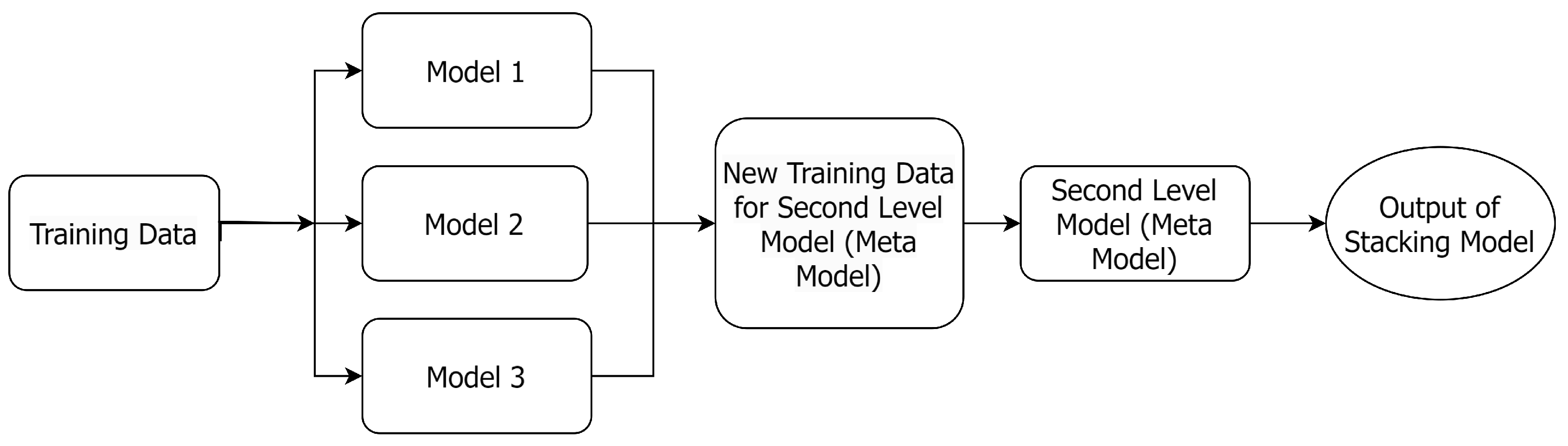
2.2. Ensemble Learning
2.3. Ensemble Learning for Anomaly Detection
2.4. Hyperspectral Unmixing-Based Voting Ensemble Anomaly Detector (HUE-AD)
3. Materials and Methods
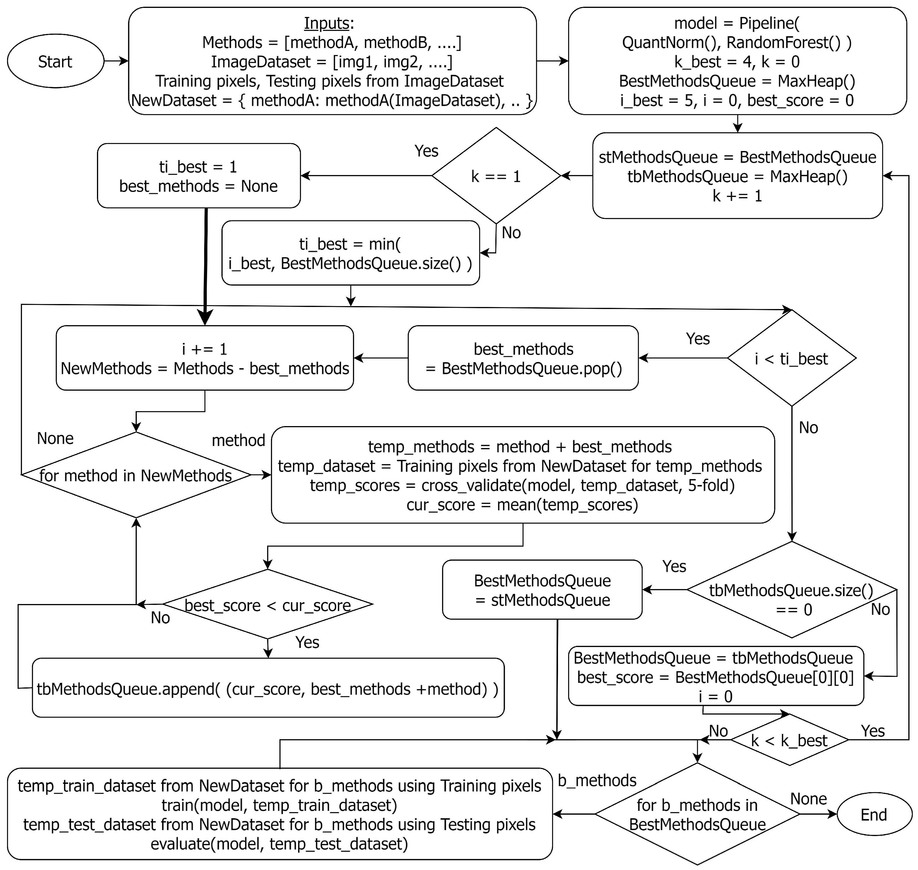
3.1. Greedy Ensemble Hyperspectral Anomaly Detector (GE-AD)
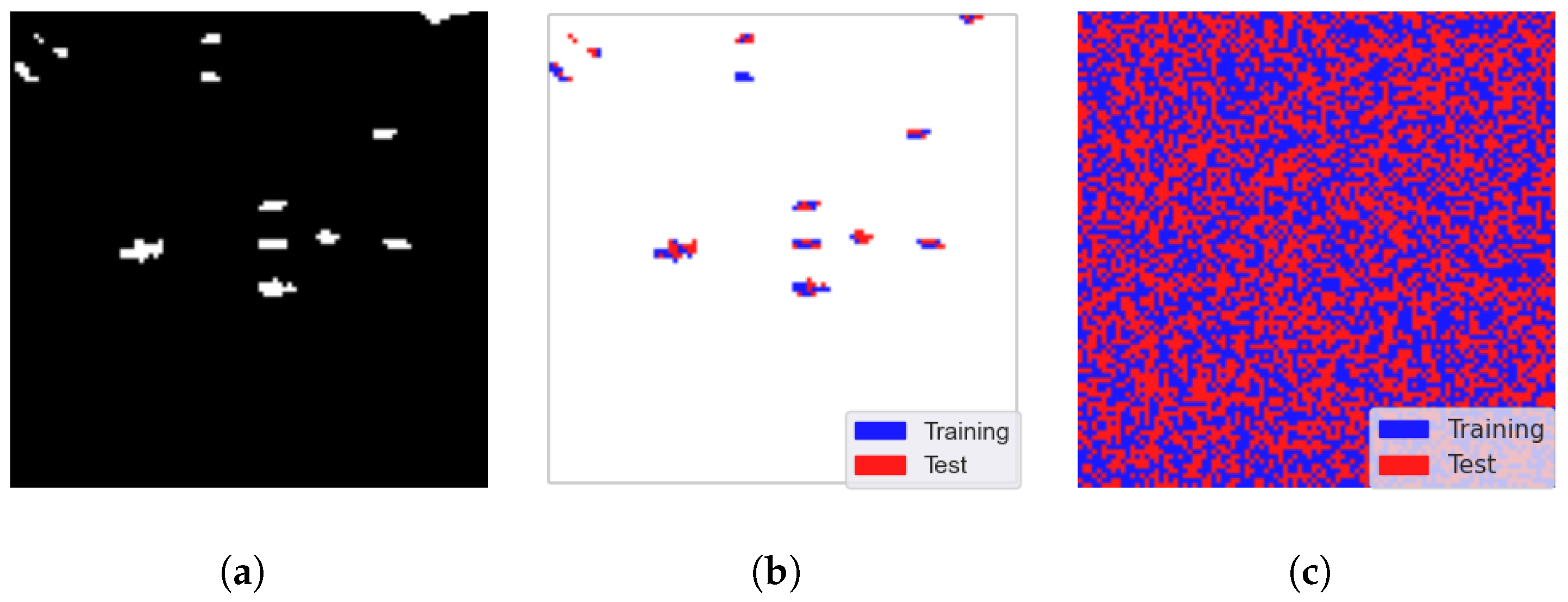
3.2. Datasets
3.3. Evaluation Metrics
3.4. Median-Based Anomaly Detector
3.5. Anomaly Detection Results Normalization
3.6. Software Tools and Development
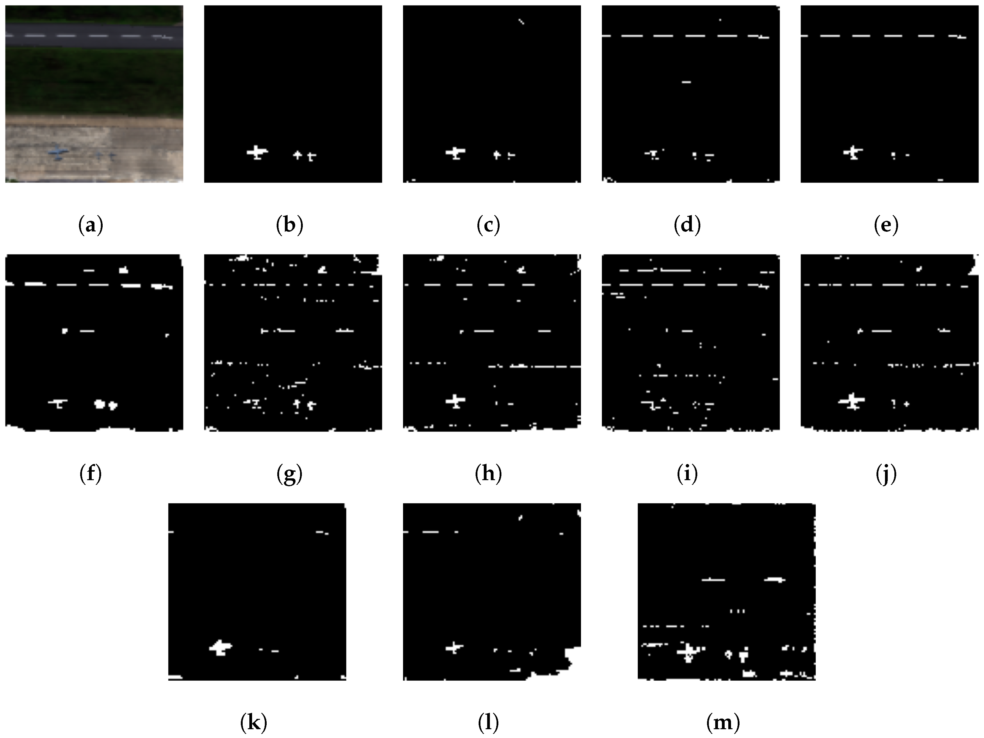
4. Results
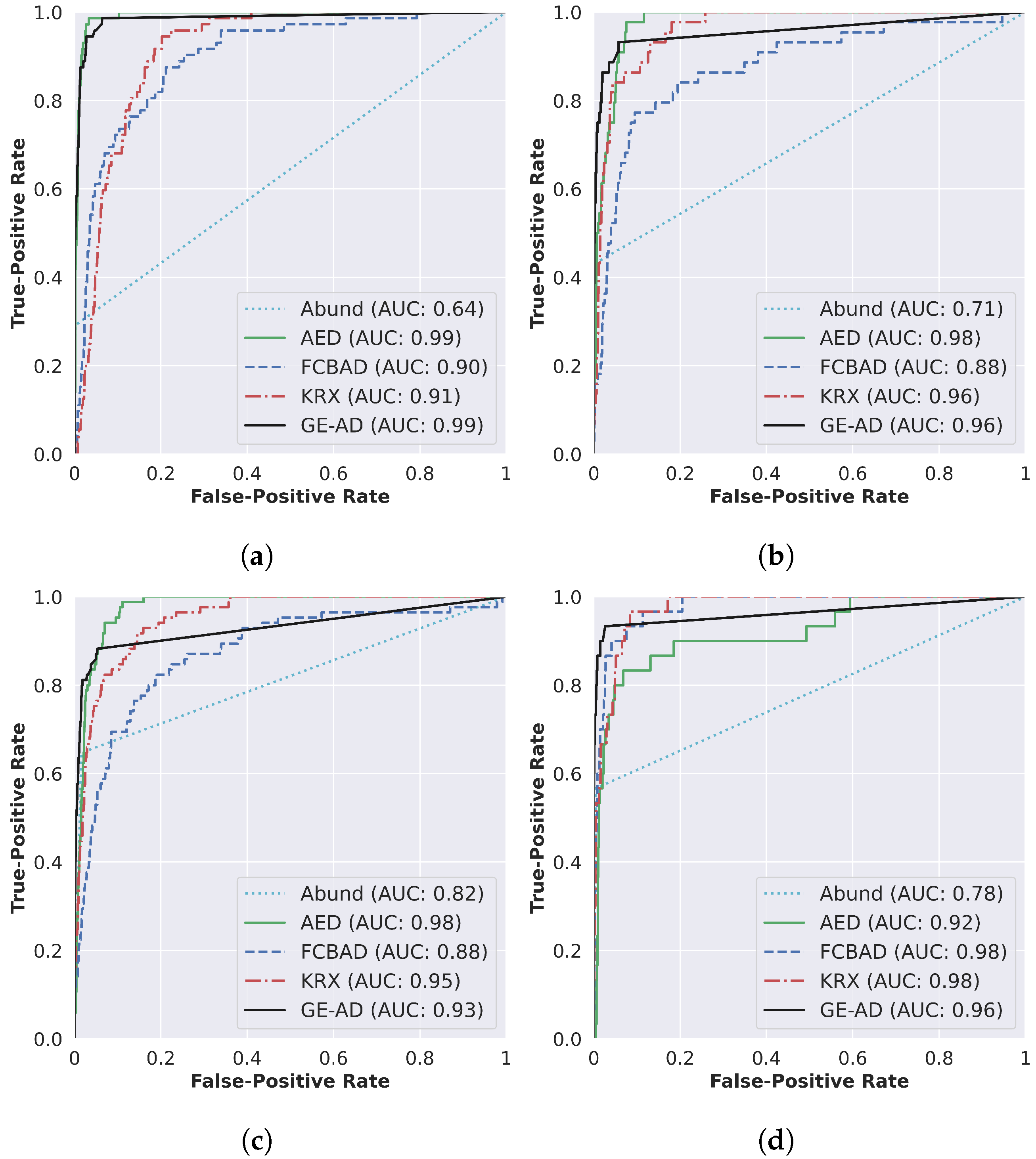
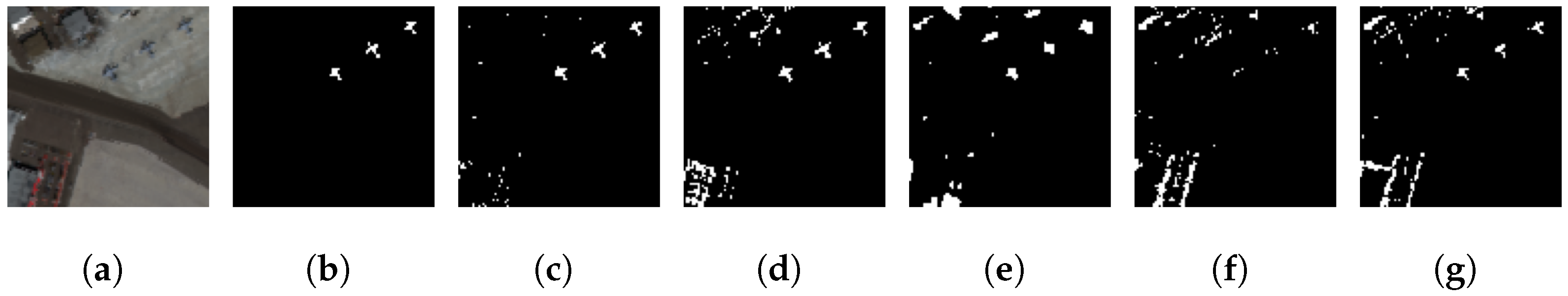
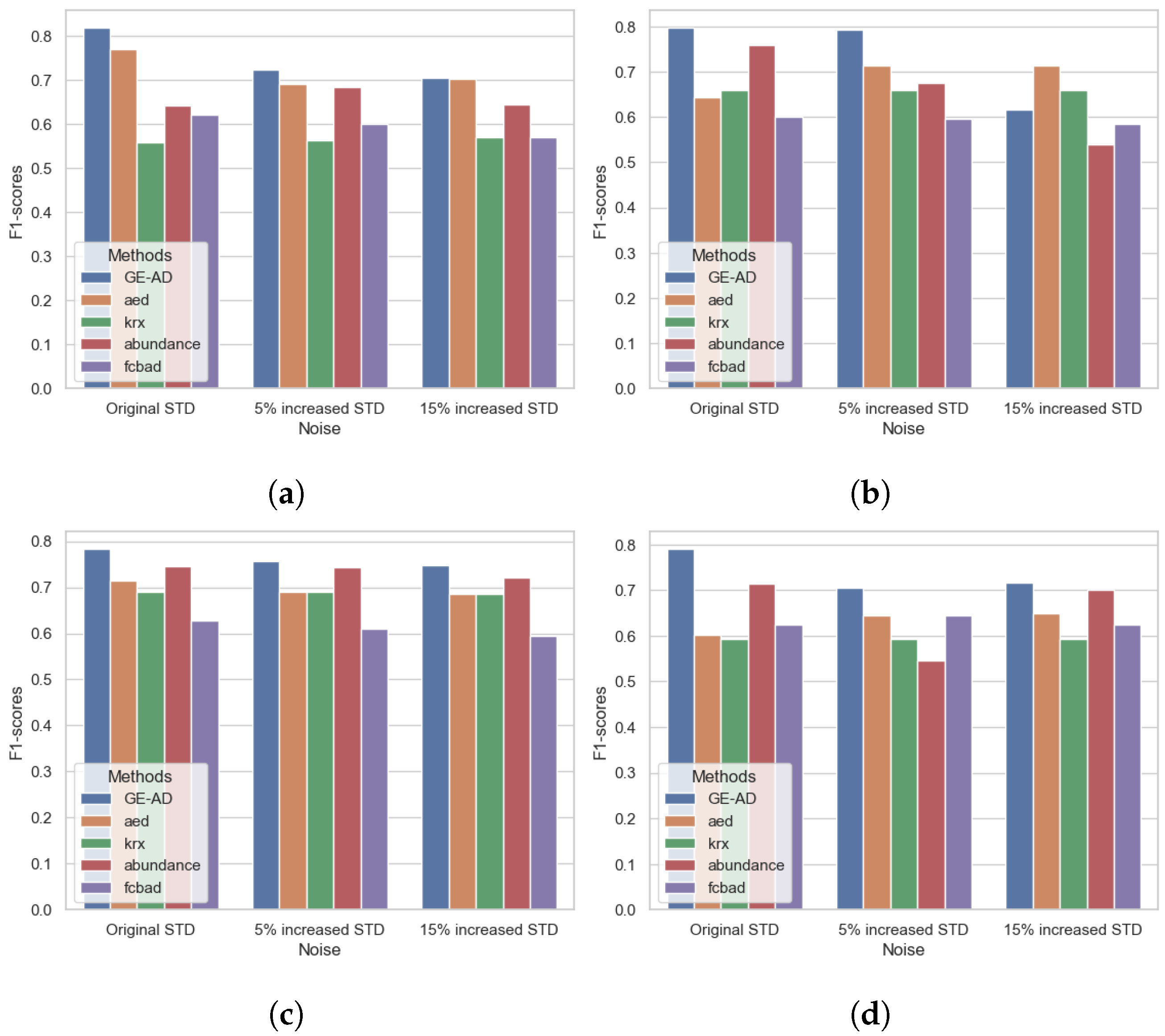
4.1. Public Dataset Benchmark Evaluation: ABU
4.1.1. Comparison with Baseline SOTA Ensemble Methods
4.1.2. Generalization Investigation: San Diego Airport
4.1.3. Ablation Study
4.2. Public Dataset Benchmark Evaluation: Hydice Urban
4.3. Public Dataset Benchmark Evaluation: Salinas
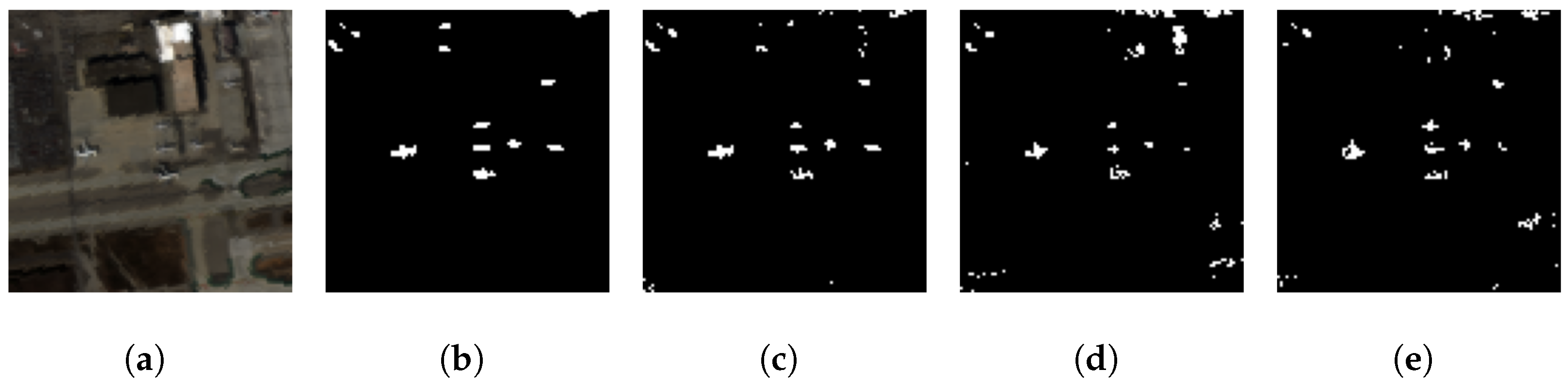
4.4. Public Dataset Benchmark Evaluation: San Diego Airport
4.5. Private Dataset Benchmark Evaluation: Arizona
5. Discussion
6. Conclusions
Supplementary Materials
Author Contributions
Funding
Institutional Review Board Statement
Informed Consent Statement
Data Availability Statement
Acknowledgments
Conflicts of Interest
References
- Manolakis, D.G.; Lockwood, R.B.; Cooley, T.W. Hyperspectral Imaging Remote Sensing: Physics, Sensors, and Algorithms; Cambridge University Press: Cambridge, UK, 2016. [Google Scholar]
- Khan, M.J.; Khan, H.S.; Yousaf, A.; Khurshid, K.; Abbas, A. Modern trends in hyperspectral image analysis: A review. IEEE Access 2018, 6, 14118–14129. [Google Scholar] [CrossRef]
- Paoletti, M.; Haut, J.; Plaza, J.; Plaza, A. Deep learning classifiers for hyperspectral imaging: A review. ISPRS J. Photogramm. Remote Sens. 2019, 158, 279–317. [Google Scholar] [CrossRef]
- Adão, T.; Hruška, J.; Pádua, L.; Bessa, J.; Peres, E.; Morais, R.; Sousa, J.J. Hyperspectral imaging: A review on UAV-based sensors, data processing and applications for agriculture and forestry. Remote Sens. 2017, 9, 1110. [Google Scholar] [CrossRef]
- Stein, D.W.; Beaven, S.G.; Hoff, L.E.; Winter, E.M.; Schaum, A.P.; Stocker, A.D. Anomaly detection from hyperspectral imagery. IEEE Signal Process. Mag. 2002, 19, 58–69. [Google Scholar] [CrossRef]
- Racetin, I.; Krtalić, A. Systematic review of anomaly detection in hyperspectral remote sensing applications. Appl. Sci. 2021, 11, 4878. [Google Scholar] [CrossRef]
- Su, H.; Wu, Z.; Zhang, H.; Du, Q. Hyperspectral anomaly detection: A survey. IEEE Geosci. Remote Sens. Mag. 2021, 10, 64–90. [Google Scholar] [CrossRef]
- Hu, X.; Xie, C.; Fan, Z.; Duan, Q.; Zhang, D.; Jiang, L.; Wei, X.; Hong, D.; Li, G.; Zeng, X.; et al. Hyperspectral anomaly detection using deep learning: A review. Remote Sens. 2022, 14, 1973. [Google Scholar] [CrossRef]
- Xu, Y.; Zhang, L.; Du, B.; Zhang, L. Hyperspectral anomaly detection based on machine learning: An overview. IEEE J. Sel. Top. Appl. Earth Obs. Remote Sens. 2022, 15, 3351–3364. [Google Scholar] [CrossRef]
- Chang, C.I.; Chiang, S.S. Anomaly detection and classification for hyperspectral imagery. IEEE Trans. Geosci. Remote Sens. 2002, 40, 1314–1325. [Google Scholar] [CrossRef]
- Kwon, H.; Nasrabadi, N.M. Kernel RX-algorithm: A nonlinear anomaly detector for hyperspectral imagery. IEEE Trans. Geosci. Remote Sens. 2005, 43, 388–397. [Google Scholar] [CrossRef]
- Acito, N.; Diani, M.; Corsini, G. Gaussian mixture model based approach to anomaly detection in multi/hyperspectral images. In Proceedings of the Image and Signal Processing for Remote Sensing XI. SPIE, San Diego, CA, USA, 31 July–4 August 2005; Volume 5982, pp. 209–217. [Google Scholar]
- Schaum, A. Joint subspace detection of hyperspectral targets. In Proceedings of the 2004 IEEE Aerospace Conference Proceedings (IEEE Cat. No. 04TH8720), Big Sky, MT, USA, 6–13 March 2004; IEEE: Piscataway, NJ, USA, 2004; Volume 3. [Google Scholar]
- Carlotto, M.J. A cluster-based approach for detecting man-made objects and changes in imagery. IEEE Trans. Geosci. Remote Sens. 2005, 43, 374–387. [Google Scholar] [CrossRef]
- Hytla, P.C.; Hardie, R.C.; Eismann, M.T.; Meola, J. Anomaly detection in hyperspectral imagery: Comparison of methods using diurnal and seasonal data. J. Appl. Remote Sens. 2009, 3, 033546. [Google Scholar] [CrossRef]
- Kang, X.; Zhang, X.; Li, S.; Li, K.; Li, J.; Benediktsson, J.A. Hyperspectral anomaly detection with attribute and edge-preserving filters. IEEE Trans. Geosci. Remote Sens. 2017, 55, 5600–5611. [Google Scholar] [CrossRef]
- Li, S.; Zhang, K.; Duan, P.; Kang, X. Hyperspectral anomaly detection with kernel isolation forest. IEEE Trans. Geosci. Remote Sens. 2019, 58, 319–329. [Google Scholar] [CrossRef]
- Tan, K.; Hou, Z.; Wu, F.; Du, Q.; Chen, Y. Anomaly detection for hyperspectral imagery based on the regularized subspace method and collaborative representation. Remote Sens. 2019, 11, 1318. [Google Scholar] [CrossRef]
- Zhao, R.; Du, B.; Zhang, L. A robust nonlinear hyperspectral anomaly detection approach. IEEE J. Sel. Top. Appl. Earth Obs. Remote Sens. 2014, 7, 1227–1234. [Google Scholar] [CrossRef]
- Raza Shah, N.; Maud, A.R.M.; Bhatti, F.A.; Ali, M.K.; Khurshid, K.; Maqsood, M.; Amin, M. Hyperspectral anomaly detection: A performance comparison of existing techniques. Int. J. Digit. Earth 2022, 15, 2078–2125. [Google Scholar] [CrossRef]
- Zhao, R.; Shi, Z.; Zou, Z.; Zhang, Z. Ensemble-based cascaded constrained energy minimization for hyperspectral target detection. Remote Sens. 2019, 11, 1310. [Google Scholar] [CrossRef]
- Lu, Y.; Zheng, X.; Xin, H.; Tang, H.; Wang, R.; Nie, F. Ensemble and random collaborative representation-based anomaly detector for hyperspectral imagery. Signal Process. 2023, 204, 108835. [Google Scholar] [CrossRef]
- Merrill, N.; Olson, C.C. Unsupervised ensemble-kernel principal component analysis for hyperspectral anomaly detection. In Proceedings of the IEEE/CVF Conference on Computer Vision and Pattern Recognition Workshops, Seattle, WA, USA, 14–19 June 2020; pp. 112–113. [Google Scholar]
- Gurram, P.; Kwon, H.; Han, T. Sparse kernel-based hyperspectral anomaly detection. IEEE Geosci. Remote Sens. Lett. 2012, 9, 943–947. [Google Scholar] [CrossRef]
- Yang, X.; Huang, X.; Zhu, M.; Xu, S.; Liu, Y. Ensemble and random RX with multiple features anomaly detector for hyperspectral image. IEEE Geosci. Remote Sens. Lett. 2022, 19, 1–5. [Google Scholar] [CrossRef]
- Wang, S.; Feng, W.; Quan, Y.; Bao, W.; Dauphin, G.; Gao, L.; Zhong, X.; Xing, M. Subfeature Ensemble-Based Hyperspectral Anomaly Detection Algorithm. IEEE J. Sel. Top. Appl. Earth Obs. Remote Sens. 2022, 15, 5943–5952. [Google Scholar] [CrossRef]
- Li, L.; Li, W.; Qu, Y.; Zhao, C.; Tao, R.; Du, Q. Prior-based tensor approximation for anomaly detection in hyperspectral imagery. IEEE Trans. Neural Networks Learn. Syst. 2020, 33, 1037–1050. [Google Scholar] [CrossRef] [PubMed]
- Younis, M.S.; Hossain, M.; Robinson, A.L.; Wang, L.; Preza, C. Hyperspectral unmixing-based anomaly detection. In Proceedings of the Computational Imaging VII. SPIE, Orlando, FL, USA, 30 April–5 May 2023; Volume 12523, p. 1252302. [Google Scholar]
- Chein-I Chang and Qian Du Estimation of number of spectrally distinct signal sources in hyperspectral imagery. IEEE Trans. Geosci. Remote. Sens. 2004, 42, 608–619. [CrossRef]
- Michael, E. Winter N-FINDR: An algorithm for fast autonomous spectral end-member determination in hyperspectral data. In Proceedings of the Imaging Spectrometry V. SPIE, Orlando, FL, USA, 18 July 1999; Volume 3753, pp. 266–275. [Google Scholar]
- Keshava, N.; Mustard, J.F. Spectral unmixing. IEEE Signal Process. Mag. 2002, 19, 44–57. [Google Scholar] [CrossRef]
- Chang, C.I. An information-theoretic approach to spectral variability, similarity, and discrimination for hyperspectral image analysis. IEEE Trans. Inf. Theory 2000, 46, 1927–1932. [Google Scholar] [CrossRef]
- Baldridge, A.M.; Hook, S.J.; Grove, C.; Rivera, G. The ASTER spectral library version 2.0. Remote Sens. Environ. 2009, 113, 711–715. [Google Scholar] [CrossRef]
- Meerdink, S.K.; Hook, S.J.; Roberts, D.A.; Abbott, E.A. The ECOSTRESS spectral library version 1.0. Remote Sens. Environ. 2019, 230, 111196. [Google Scholar] [CrossRef]
- Opitz, J.; Burst, S. Macro f1 and macro f1. arXiv 2019, arXiv:1911.03347. [Google Scholar]
- Reed, I.S.; Yu, X. Adaptive multiple-band CFAR detection of an optical pattern with unknown spectral distribution. IEEE Trans. Acoust. Speech Signal Process. 1990, 38, 1760–1770. [Google Scholar] [CrossRef]
- Mahalanobis, P.C. On the generalized distance in statistics. Sankhyā Indian J. Stat. Ser. A (2008-) 2018, 80, S1–S7. [Google Scholar]
- Du, B.; Zhao, R.; Zhang, L.; Zhang, L. A spectral-spatial based local summation anomaly detection method for hyperspectral images. Signal Process. 2016, 124, 115–131. [Google Scholar] [CrossRef]
- Liu, F.T.; Ting, K.M.; Zhou, Z.-H. Isolation forest. In Proceedings of the 2008 Eighth IEEE International Conference on Data Mining, Pisa, Italy, 15–19 December 2008; Volume 1, pp. 413–422. [Google Scholar]
- Wolpert, D.H. Stacked generalization. Neural Netw. 1992, 5, 241–259. [Google Scholar] [CrossRef]
- Pavlyshenko, B. Using stacking approaches for machine learning models. In Proceedings of the 2018 IEEE Second International Conference on Data Stream Mining & Processing (DSMP), Lviv, Ukraine, 21–25 August 2018; IEEE: Piscataway, NJ, USA, 2018; pp. 255–258. [Google Scholar]
- Fatemifar, S.; Awais, M.; Akbari, A.; Kittler, J. A stacking ensemble for anomaly based client-specific face spoofing detection. In Proceedings of the 2020 IEEE International Conference on Image Processing (ICIP), Abu Dhabi, United Arab Emirates, 25–28 October 2020; IEEE: Piscataway, NJ, USA, 2020; pp. 1371–1375. [Google Scholar]
- Nalepa, J.; Myller, M.; Tulczyjew, L.; Kawulok, M. Deep ensembles for hyperspectral image data classification and unmixing. Remote Sens. 2021, 13, 4133. [Google Scholar] [CrossRef]
- Zhang, X.; Zhao, H. Hyperspectral-cube-based mobile face recognition: A comprehensive review. Inf. Fusion 2021, 74, 132–150. [Google Scholar] [CrossRef]
- Seni, G.; Elder, J. Ensemble Methods in Data Mining: Improving Accuracy through Combining Predictions; Morgan & Claypool Publishers: Williston, VT, USA, 2010. [Google Scholar]
- Aggarwal, C.C.; Sathe, S. Theoretical foundations and algorithms for outlier ensembles. ACM Sigkdd Explor. Newsl. 2015, 17, 24–47. [Google Scholar] [CrossRef]
- De Tchébychef, P. Average values. J. Pure Appl. Math. 1867, 12, 177–184. [Google Scholar]
- Breiman, L. Stacked regressions. Mach. Learn. 1996, 24, 49–64. [Google Scholar] [CrossRef]
- Sill, J.; Takács, G.; Mackey, L.; Lin, D. Feature-weighted linear stacking. arXiv 2009, arXiv:0911.0460. [Google Scholar]
- Cox, D.R. The regression analysis of binary sequences. J. R. Stat. Soc. Ser. B Stat. Methodol. 1958, 20, 215–232. [Google Scholar] [CrossRef]
- Quinlan, J.R. C4. 5: Programs for Machine Learning; Elsevier: Amsterdam, The Netherlands, 2014. [Google Scholar]
- Breiman, L. Random forests. Mach. Learn. 2001, 45, 5–32. [Google Scholar] [CrossRef]
- Fushiki, T. Estimation of prediction error by using K-fold cross-validation. Stat. Comput. 2011, 21, 137–146. [Google Scholar] [CrossRef]
- Anguita, D.; Ghelardoni, L.; Ghio, A.; Oneto, L.; Ridella, S. The’K’in K-fold Cross Validation. In Proceedings of the ESANN, Bruges, Belgium, 25–27 April 2012; pp. 441–446. [Google Scholar]
- Wong, T.T.; Yeh, P.Y. Reliable accuracy estimates from k-fold cross validation. IEEE Trans. Knowl. Data Eng. 2019, 32, 1586–1594. [Google Scholar] [CrossRef]
- Kang, X. Airport-Beach-Urban (ABU) Datasets. 2017. Available online: http://xudongkang.weebly.com/data-sets.html (accessed on 23 April 2023).
- Zhao, Y.Q.; Yang, J. Hyperspectral image denoising via sparse representation and low-rank constraint. IEEE Trans. Geosci. Remote Sens. 2014, 53, 296–308. [Google Scholar] [CrossRef]
- Zhu, L.; Wen, G. Hyperspectral anomaly detection via background estimation and adaptive weighted sparse representation. Remote Sens. 2018, 10, 272. [Google Scholar] [CrossRef]
- Graña, M.; Veganzons, M.A.; Ayerdi, B. Hyperspectral Remote Sensing Scenes; University of the Basque Country: Basque, Spanish, 2021. Available online: https://www.ehu.eus/ccwintco/index.php/Hyperspectral_Remote_Sensing_Scenes (accessed on 13 January 2024).
- Li, W.; Wu, G.; Du, Q. Transferred Deep Learning for Anomaly Detection in Hyperspectral Imagery; Git Hub: San Francisco, CA, USA, 2017; Available online: https://github.com/yousefan/CNND/blob/master/HYDICE_urban.mat (accessed on 13 January 2024).
- Watson, T.P.; McKenzie, K.; Robinson, A.; Renshaw, K.; Driggers, R.; Jacobs, E.L.; Conroy, J. Evaluation of aerial real-time RX anomaly detection. In Proceedings of the Algorithms, Technologies, and Applications for Multispectral and Hyperspectral Imaging XXIX. SPIE, Orlando, FL, USA, 30 April–5 May 2023; Volume 12519, pp. 254–260. [Google Scholar]
- AVIRIS—Airborne Visible/Infrared Imaging Spectrometer. Available online: https://aviris.jpl.nasa.gov/ (accessed on 23 January 2024).
- Liu, X.; Tanaka, M.; Okutomi, M. Single-image noise level estimation for blind denoising. IEEE Trans. Image Process. 2013, 22, 5226–5237. [Google Scholar] [CrossRef] [PubMed]
- Army Geospatial Center. Available online: https://www.agc.army.mil/ (accessed on 22 April 2024).
- Basedow, R.; Zalewski, E. Characteristics of the HYDICE sensor. In Proceedings of the Summaries of the Fifth Annual JPL Airborne Earth Science Workshop, Pasadena, CA, USA, 23–26 January 1995; AVIRIS Workshop: Pasadena, CA, USA, 1995; Volume 1, p. 9. [Google Scholar]
- Pika L—Hyperspectral Sensors—Lightweight, Compact VNIR—Benchtop Systems—Resonon. Available online: https://resonon.com/Pika-L (accessed on 13 September 2023).
- Hanley, J.A.; McNeil, B.J. The meaning and use of the area under a receiver operating characteristic (ROC) curve. Radiology 1982, 143, 29–36. [Google Scholar] [CrossRef] [PubMed]
- Chang, C.I. Comprehensive Analysis of Receiver Operating Characteristic (ROC) Curves for Hyperspectral Anomaly Detection. IEEE Trans. Geosci. Remote Sens. 2022, 60, 1–24. [Google Scholar] [CrossRef]
- GeeksforGeeks. AUC ROC Curve in Machine Learning. Available online: https://www.geeksforgeeks.org/auc-roc-curve/ (accessed on 13 January 2024).
- Chinchor, N. MUC-4 Evaluation Metrics. In Proceedings of the MUC4 ’92: 4th Conference on Message Understanding, Stroudsburg, PA, USA, 16–18 June 1992; pp. 22–29. [Google Scholar] [CrossRef]
- Saito, T.; Rehmsmeier, M. The precision-recall plot is more informative than the ROC plot when evaluating binary classifiers on imbalanced datasets. PLoS ONE 2015, 10, e0118432. [Google Scholar] [CrossRef]
- Tamersoy, B. Background Subtraction; The University of Texas at Austin: Austin, TX, USA, 2009. [Google Scholar]
- Du, Q.; Yang, H. Similarity-based unsupervised band selection for hyperspectral image analysis. IEEE Geosci. Remote Sens. Lett. 2008, 5, 564–568. [Google Scholar] [CrossRef]
- Kriegel, H.P.; Kroger, P.; Schubert, E.; Zimek, A. Interpreting and unifying outlier scores. In Proceedings of the 2011 SIAM International Conference on Data Mining, Mesa, AZ, USA, 28–30 April 2011; pp. 13–24. [Google Scholar]
- Aggarwal, C.C. Outlier ensembles: Position paper. ACM SIGKDD Explor. Newsl. 2013, 14, 49–58. [Google Scholar] [CrossRef]
- Zimek, A.; Campello, R.J.; Sander, J. Ensembles for unsupervised outlier detection: Challenges and research questions a position paper. ACM Sigkdd Explor. Newsl. 2014, 15, 11–22. [Google Scholar] [CrossRef]
- Välikangas, T.; Suomi, T.; Elo, L.L. A systematic evaluation of normalization methods in quantitative label-free proteomics. Briefings Bioinform. 2018, 19, 1–11. [Google Scholar] [CrossRef] [PubMed]
- Zhao, Y.; Wong, L.; Goh, W.W.B. How to do quantile normalization correctly for gene expression data analyses. Sci. Rep. 2020, 10, 15534. [Google Scholar] [CrossRef] [PubMed]
- Zare, A.; Glenn, T.; Gader, P. GatorSense Hyperspectral Image Analysis Toolkit; Version 0.1; Zenodo: Honolulu, HI, USA, 2018. [Google Scholar] [CrossRef]
- Lyngdoh, R.B.; Sahadevan, A.S.; Ahmad, T.; Rathore, P.S.; Mishra, M.; Gupta, P.K.; Misra, A. Avhyas: A free and open source qgis plugin for advanced hyperspectral image analysis. In Proceedings of the 2021 International Conference on Emerging Techniques in Computational Intelligence (ICETCI), Hyderabad, India, 25–27 August 2021; IEEE: Piscataway, NJ, USA, 2021; pp. 71–76. [Google Scholar]
- Project, O.S.G.F. QGIS Geographic Information System, Version 3.14.1; QGIS: London, UK, 2020. Available online: http://qgis.org (accessed on 19 August 2023).
- Pedregosa, F.; Varoquaux, G.; Gramfort, A.; Michel, V.; Thirion, B.; Grisel, O.; Blondel, M.; Prettenhofer, P.; Weiss, R.; Dubourg, V.; et al. Scikit-learn: Machine Learning in Python. J. Mach. Learn. Res. 2011, 12, 2825–2830. [Google Scholar]
- Wilcoxon, F. Individual Comparisons by Ranking Methods. Biom. Bull. 1945, 1, 80–83. [Google Scholar] [CrossRef]
- Mann, H.B.; Whitney, D.R. On a test of whether one of two random variables is stochastically larger than the other. Ann. Math. Stat. 1947, 18, 50–60. [Google Scholar] [CrossRef]
- Student. The probable error of a mean. Biometrika 1908, 6, 1–25. [Google Scholar] [CrossRef]
- Friedman, M. The use of ranks to avoid the assumption of normality implicit in the analysis of variance. J. Am. Stat. Assoc. 1937, 32, 675–701. [Google Scholar] [CrossRef]
- DeLong, E.R.; DeLong, D.M.; Clarke-Pearson, D.L. Comparing the areas under two or more correlated receiver operating characteristic curves: A nonparametric approach. Biometrics 1988, 44, 837–845. [Google Scholar] [CrossRef]
- Krzanowski, W.J.; Hand, D.J. ROC Curves for Continuous Data; CRC: Boca Raton, FL, USA; Chapman and Hall: London, UK, 2009. [Google Scholar]
- Statistical Significance (p-Value) for Comparing Two Classifiers with Respect to (Mean) ROC AUC, Sensitivity and Specificity. Cross Validated. 2018. Available online: https://stats.stackexchange.com/q/358598 (accessed on 10 April 2024).
- Shorten, C.; Khoshgoftaar, T.M. A survey on image data augmentation for deep learning. J. Big Data 2019, 6, 1–48. [Google Scholar] [CrossRef]
- Maharana, K.; Mondal, S.; Nemade, B. A review: Data pre-processing and data augmentation techniques. Glob. Transitions Proc. 2022, 3, 91–99. [Google Scholar] [CrossRef]
- Hidalgo, J.A.P.; Pérez-Suay, A.; Nar, F.; Camps-Valls, G. Efficient nonlinear RX anomaly detectors. IEEE Geosci. Remote Sens. Lett. 2020, 18, 231–235. [Google Scholar] [CrossRef]
- Chicco, D.; Jurman, G. The advantages of the Matthews correlation coefficient (MCC) over F1 score and accuracy in binary classification evaluation. BMC Genom. 2020, 21, 6. [Google Scholar] [CrossRef] [PubMed]
- Boggs, T.; March, D.; Kormang; McGibbney, L.J.; Magimel, F.; Mason, G.; Banman, K.; Kumar, R.; Badger, T.G.; Aarnio, T.; et al. Spectralpython/Spectral: Spectral Python (SPy), 0.22.4. Zenodo: Honolulu, HI, USA, 2021. [Google Scholar] [CrossRef]


| Literature | Base Models | Type of Base Models | Base Model Optimization | Base Model Selection | Aggregation |
|---|---|---|---|---|---|
| ERCRD [22] | homogeneous | unsupervised | random sampling | N/A | bagging, summation |
| UE-kPCA [23] | homogeneous | unsupervised | random sampling, gradient descent optimization | N/A | bagging, average |
| ERRX MFs [25] | heterogeneous, mixed with passthrough | unsupervised | random sampling | not mentioned | bagging, average |
| SED [26] | only one method or heterogeneous, mixed with passthrough | unsupervised | not mentioned | based on ensemble performance | stacking, unsupervised meta method |
| Fatemifar et al. [42] | heterogeneous | unsupervised | not mentioned | genetic algorithm | stacking, unsupervised meta method |
| Nalepa et al. [43] | heterogeneous | supervised | not optimized | not investigated | stacking, supervised meta-learner |
| HUE-AD [28] | heterogeneous | unsupervised | not optimized | based on individual performance | bagging, voting |
| GE-AD | heterogeneous | unsupervised | not optimized | greedy search | stacking, supervised meta-learner |
| Percentile Values | Image I | Image II | Image III | Image IV | Image V |
|---|---|---|---|---|---|
| 0.90 | 0.506 | 0.534 | 0.586 | 0.486 | 0.595 |
| 0.95 | 0.516 | 0.562 | 0.630 | 0.503 | 0.643 |
| 0.97 | 0.519 | 0.575 | 0.650 | 0.513 | 0.670 |
| Datasets | Base Models | Training Score | Training Time (s) | Test Score | Inference Time (s) |
|---|---|---|---|---|---|
| ABU | Abundance, AED, FCBAD, KRX | 87.901 | 1.498 | ||
| Hydice Urban | FCBAD, LSUNRSORAD | 25.156 | 0.464 | ||
| Salinas | LSUNRSORAD | 20.657 | 0.494 | ||
| San Diego Airport | Abundance, GMRX, KIFD, KRX | 47.681 | 0.902 | ||
| Arizona | FCBAD, KIFD, KRX, LSUNRSORAD | 2983.433 | 24.037 |
| Method | Avg. F1-Macro Score | Wilcoxon’s p-Value [83] |
|---|---|---|
| GE-AD | 86.452 | |
| Abundance [31] | 73.11 | 3.2748 × 10⁻¹⁴ |
| AED [16] | 65.282 | 3.9248 × 10⁻¹⁵ |
| FCBAD [15] | 59.253 | 3.9248 × 10⁻¹⁵ |
| GMRX [12] | 55.453 | 3.9248 × 10⁻¹⁵ |
| KIFD [17] | 64.657 | 3.9244 × 10⁻¹⁵ |
| KRX [11] | 61.535 | 3.9248 × 10⁻¹⁵ |
| LSUNRSORAD [18] | 61.058 | 3.9248 × 10⁻¹⁵ |
| Method | ABU-I | ABU-II | ABU-III | ABU-IV | Avg. F1 -Macro Score | Wilcoxon’s p-Value [83] | Avg. Rank | Friedman’s p-Value [86] |
|---|---|---|---|---|---|---|---|---|
| GE-AD | 0.887 | 0.878 | 0.875 | 0.769 | 1.07 | 3.397 × 10⁻²⁶ | ||
| HUE-AD [28] | 0.793 | 0.770 | 0.751 | 0.649 | 1.9262 × 10⁻⁸ | 2.62 | ||
| Abundance [31] | 0.670 | 0.741 | 0.760 | 0.736 | 3.033 × 10⁻⁸ | 3.10 | ||
| AED [16] | 0.781 | 0.646 | 0.697 | 0.610 | 1.7847 × 10⁻⁸ | 4.40 | ||
| FCBAD [15] | 0.606 | 0.603 | 0.591 | 0.621 | 1.7847 × 10⁻⁸ | 6.75 | ||
| KIFD [17] | 0.694 | 0.682 | 0.695 | 0.587 | 1.7847 × 10⁻⁸ | 5.05 | ||
| KRX [11] | 0.559 | 0.658 | 0.659 | 0.604 | 1.7847 × 10⁻⁸ | 6.42 | ||
| LSUNRSORAD [18] | 0.695 | 0.608 | 0.661 | 0.568 | 1.7847 × 10⁻⁸ | 6.58 |
| Method | ABU-I | ABU-II | ABU-III | ABU-IV | Avg. AUC Score | Wilcoxon’s p-Value [83] | Avg. Rank | Friedman’s p-Value [86] |
|---|---|---|---|---|---|---|---|---|
| GE-AD | 0.987 | 0.980 | 0.975 | 0.978 | 2.00 | 3.901 × 10⁻²² | ||
| Abundance | 0.620 | 0.733 | 0.834 | 0.805 | 1.7847 × 10⁻⁸ | 7.15 | ||
| AED | 0.992 | 0.980 | 0.975 | 0.932 | 3.8011 × 10⁻² | 2.48 | ||
| FCBAD | 0.900 | 0.896 | 0.889 | 0.978 | 1.4139 × 10⁻⁷ | 4.28 | ||
| KRX | 0.914 | 0.971 | 0.951 | 0.975 | 2.7606 × 10⁻⁵ | 3.55 |
| GE-AD | ERRX MF [25] | ERCRD [22] | SED [26] | |
|---|---|---|---|---|
| ROC AUC score | 0.9632 | 0.9970 | 0.9533 | 0.9980 |
| F1-macro score | 0.856 | 0.666 | 0.545 | 0.592 |
| ABU-I | ABU-II | ABU-III | ABU-IV | |
|---|---|---|---|---|
| AED, KRX, Abundance | 0.797 | 0.764 | 0.835 | 0.754 |
| AED, KRX, Abundance, FCBAD | 0.807 | 0.788 | 0.784 | 0.856 |
| All nine methods | 0.824 | 0.810 | 0.779 | 0.768 |
| Method | Abundance | AED | CSD | FCBAD | GMRX | KIFD | KRX | LSUNRSORAD | RX |
|---|---|---|---|---|---|---|---|---|---|
| Running Time (s) | 6.2495 | 22.8803 | 0.42967 | 35.2065 | 3.8688 | 48.1669 | 138.821 | 20.741 | 0.37361 |
| Method | Avg. F1-Macro Score | Wilcoxon’s p-Value [83] | Avg. Rank |
|---|---|---|---|
| GE-AD | 1.00 | ||
| FCBAD | 9.7656 × 10⁻⁴ | 2.20 | |
| LSUNRSORAD | 9.7656 × 10⁻⁴ | 2.80 |
| Method | Avg. F1-Macro Score | Wilcoxon’s p-Value [83] | Avg. Rank |
|---|---|---|---|
| GE-AD | 1.00 | ||
| LSUNRSORAD | 9.7656 × 10⁻⁴ | 2.00 |
| Method | San Diego-01 | San Diego-02 | Avg. F1 -Macro Score | Wilcoxon’s p-Value [83] | Avg. Rank |
|---|---|---|---|---|---|
| GE-AD | 0.883 | 0.910 | 1.00 | ||
| Abundance | 0.790 | 0.655 | 9.5367 × 10⁻⁷ | 2.20 | |
| GMRX | 0.552 | 0.497 | 9.5367 × 10⁻⁷ | 5.00 | |
| KIFD | 0.774 | 0.642 | 9.5367 × 10⁻⁷ | 2.80 | |
| KRX | 0.714 | 0.627 | 9.5367 × 10⁻⁷ | 4.00 |
| Method | Arizona-I | Arizona-II | Arizona-III | Arizona-IV | Arizona-V | Avg. F1 -Macro Score | Wilcoxon’s p-Value [83] | Avg. Rank | Friedman’s p-Value [86] |
|---|---|---|---|---|---|---|---|---|---|
| GE-AD | 0.770 | 0.799 | 0.882 | 0.816 | 0.859 | 1.00 | 3.465 × 10⁻²⁹ | ||
| FCBAD [15] | 0.587 | 0.614 | 0.774 | 0.542 | 0.812 | 3.7785 × 10⁻¹⁰ | 2.40 | ||
| KIFD [17] | 0.570 | 0.569 | 0.584 | 0.505 | 0.578 | 3.7785 × 10⁻¹⁰ | 3.96 | ||
| KRX [11] | 0.633 | 0.675 | 0.494 | 0.514 | 0.503 | 3.7785 × 10⁻¹⁰ | 3.40 | ||
| LSUNRSORAD [18] | 0.520 | 0.571 | 0.640 | 0.498 | 0.572 | 3.7785 × 10⁻¹⁰ | 4.24 |
Disclaimer/Publisher’s Note: The statements, opinions and data contained in all publications are solely those of the individual author(s) and contributor(s) and not of MDPI and/or the editor(s). MDPI and/or the editor(s) disclaim responsibility for any injury to people or property resulting from any ideas, methods, instructions or products referred to in the content. |
© 2024 by the authors. Licensee MDPI, Basel, Switzerland. This article is an open access article distributed under the terms and conditions of the Creative Commons Attribution (CC BY) license (https://creativecommons.org/licenses/by/4.0/).
Share and Cite
Hossain, M.; Younis, M.; Robinson, A.; Wang, L.; Preza, C. Greedy Ensemble Hyperspectral Anomaly Detection. J. Imaging 2024, 10, 131. https://doi.org/10.3390/jimaging10060131
Hossain M, Younis M, Robinson A, Wang L, Preza C. Greedy Ensemble Hyperspectral Anomaly Detection. Journal of Imaging. 2024; 10(6):131. https://doi.org/10.3390/jimaging10060131
Chicago/Turabian StyleHossain, Mazharul, Mohammed Younis, Aaron Robinson, Lan Wang, and Chrysanthe Preza. 2024. "Greedy Ensemble Hyperspectral Anomaly Detection" Journal of Imaging 10, no. 6: 131. https://doi.org/10.3390/jimaging10060131
APA StyleHossain, M., Younis, M., Robinson, A., Wang, L., & Preza, C. (2024). Greedy Ensemble Hyperspectral Anomaly Detection. Journal of Imaging, 10(6), 131. https://doi.org/10.3390/jimaging10060131