Article

Variability and Bias in Measurements of Metals Mass Fractions in Automobile Shredder Residue

1
Empa, Swiss Federal Laboratories for Materials Science and Technology, Technology and Society Laboratory, CH-9014 St. Gallen, Switzerland
2
Empa, Swiss Federal Laboratories for Materials Science and Technology, Advanced Analytical Technologies, CH-8600 Dübendorf, Switzerland
3
Empa, Swiss Federal Laboratories for Materials Science and Technology, Particles-Biology Interactions Laboratory, CH-9014 St. Gallen, Switzerland
4
University of Applied Sciences Rapperswil, Institute of Environmental and Process Engineering (Umtec), CH-8640 Rapperswil, Switzerland
5
Technische Universität Berlin, Chair of Circular Economy and Recycling Technology, 10623 Berlin, Germany
*
Author to whom correspondence should be addressed.
Recycling 2019, 4(3), 34; https://doi.org/10.3390/recycling4030034
Submission received: 26 June 2019 / Revised: 6 August 2019 / Accepted: 16 August 2019 / Published: 21 August 2019

Abstract

:
The treatment of end-of-life vehicles generates large amounts of automobile shredder residue (ASR), a potential source of recycled metals. Reliable measurement methods are required to determine the composition of ASR and evaluate the resource potential. We reported on research undertaken to investigate bias and variability in the process of measuring trace metals in ASR. Two primary samples of shredder light fraction (SLF) underwent extensive physical sample preparation and chemical analysis. The samples were spiked to control random variations and systematic effects during physical sample preparation. Chemical analysis was conducted using wavelength-dispersive X-ray fluorescence spectrometry (WD-XRF), a fully validated wet-chemical analysis, and a wet-chemical analysis representing an “in-house” lab procedure. Physical sample preparation introduced deviations up to a factor of 2, likely due to preferential losses and heterogeneity. Deviations for WD-XRF measurements of elements were in the range +100%/−50%. In-house chemical analysis produced results that were in good agreement with validated results for Al, Fe and Sn, but led to biased results or high variability for Cd, Dy, La, Nd, Pb, Pd, Pt and Sb. To improve the chemical analysis of trace metals in SLF, we recommended reducing particle size to less than 0.1 mm before chemical analysis and using a larger number of repeated digestions.

Graphical Abstract

1. Introduction

Each year, more than 6 million end-of-life vehicles (ELVs) are treated in the European Union [1]. After being depolluted and dismantled, the ELV hulks are treated in shredders to mechanically liberate and separate base metals, mainly steel and aluminum, from other materials. Most other non-metallic materials, such as plastics, textiles and glass end up as waste collectively referred to as automobile shredder residue (ASR), which is usually incinerated or landfilled [2]. ASR normally contains toxic substances such as heavy metals, polychlorinated biphenyls (PCBs) and brominated flame retardants (BFRs) [3,4,5] and is considered a hazardous waste [6]. Lately, attention has turned towards its content of rare metals and their potential recovery [7,8,9,10].
The characterization of ASR is necessary to evaluate its toxicity, potential environmental impacts, secondary raw material potentials and the technical possibilities for recovering metals. Substances of interest, such as cadmium or gold, typically occur at low mass fractions only in the parts per million (ppm) range [5,8]. The low concentrations of target substances combined with the heterogeneity of the material make sampling, sample preparation and chemical analysis extremely demanding tasks.
The goal of a detailed ASR characterization is usually to determine the mass fraction or a related physical quantity of one or several substances, called the analyte(s), in a defined volume of ASR. The measured quantity will, for example, determine whether the waste is to be considered hazardous, or may be used to estimate its value as a source of metals. As it is not feasible to analyze the entire volume, the measurement process involves a series of sampling and sample preparation steps before the actual detection of the analyte. The measurement process can be divided into three phases: 1) sampling, 2) physical sample preparation and 3) chemical analysis [11].
The first phase consists in taking a sample that is likely to have a composition similar to the batch. The larger the heterogeneity of the lot with respect to the analyte, the larger the sample must be to ensure representativeness [12]. Rare metals in ASR typically originate from small car components such as permanent magnets or integrated circuits in which they are used at elevated mass fractions [8]. Unless these components are comminuted and distributed in the shredder, their distribution in the outputs is likely to be very heterogeneous. Using the theory of sampling, it is in principle possible to calculate the sample size necessary to achieve a predefined level of uncertainty related to sampling [12]. However, the theory of sampling was developed for the mining industry, and although the theoretical foundations also apply to other materials, the calculation of uncertainties and representative sample masses ultimately relies on several assumptions and the use of material-specific parameters, such as the so-called liberation factor. One study has been undertaken to adapt and validate the sampling theory for analysis of ASR [13], but only for the determination of the main constituent materials such as rubber and plastics. To our knowledge, the theory has never been validated for measuring substances at trace mass fractions in heterogeneous wastes.
For heterogeneous wastes such as ASR, the primary sample taken from the batch typically has a mass of at least several kilograms [14,15,16]. Wet-chemical analysis methods rely on digesting a few subsamples of less than 1 g each [17]. Hence, the sample size must be dramatically reduced through a series of homogenization and subsampling steps. This second phase of the measurement process is referred to as physical sample preparation [11]. Homogenization involves comminution and mixing of the material by cutting, milling, grinding or a similar operation. Such operations may introduce systematic deviations in the measurement through contaminations from the equipment or unintentional losses (For an explanation of the terms random and systematic deviations, or errors, see p. 37 in Annex B to the GUM: Guide to Expression of Uncertainty in Measurement [18].). Moreover, due to the residual heterogeneity always present in the material, each subsampling step introduces additional random deviations and may also generate systematic deviations by preferential selection of certain constituents [19].
Sample preparation of ASR is particularly challenging due to its heterogeneity and the presence of objects with entirely different physical properties. Despite its potential impact on the measurement results, sample preparation has received little attention in the waste analysis literature. Among the 21 identified studies with the aim to characterize ASR, only 11 provided basic information on the sample preparation procedure, and none involved quantification of uncertainties or bias related to this step [3,4,5,7,8,9,15,16,20,21,22,23,24,25,26,27,28,29,30,31,32,33]. In general, random deviations introduced in sample preparation may be investigated and neutralized by repetition, although at a high cost, while systematic effects (bias) may be detected by spiking the material with a tracer substance prior to sample preparation [34].
To complete the measurement process, the final test sample (e.g., 0.1 g of material) goes through a chemical analysis procedure, which is usually conducted in two steps: chemical or physical treatment followed by detection of the analyte [11]. With X-ray fluorescence spectrometry (XRF), detection may be done directly on the homogenized powder sample or on physically prepared samples such as fused beads or wax pellets. Wet-chemical analysis involves dissolving the sample in an acid or base solution before detection, e.g., with mass spectrometry or optical emission/absorption spectroscopy techniques. Like in sampling and physical sample preparation, random and systematic effects may influence the results of chemical analysis. Random deviations caused by the measurement method or residual heterogeneity in the sample lead to variability between different test samples and can to some extent be controlled by repeating the chemical analysis with independent subsamples. Systematic deviations may have various causes, including but not limited to incomplete dissolution of the matrix material, chemical reactions between the analyte and other constituents followed by precipitation or evaporation, and overlapping spectra between the analyte and other constituents. Such effects are more likely to influence the measurement when the sample contains a large variety of materials and substances, as is the case for ASR.
Control and/or elimination of all the possible effects that may influence the final measurement result would lead to very high costs and is not feasible in most projects. It is therefore of high interest to (1) identify target elements, methods or combinations thereof, for which bias is more likely to occur, (2) identify simpler analysis methods with little influence on the reliability of the result, (3) estimate typical levels of uncertainty for particular elements and/or methods. In this article, we report on work undertaken to address these three points for trace metals in ASR, specifically shredder light fraction (SLF), which constitutes the majority of ASR. We focused on the sample preparation and chemical analysis phases while acknowledging that sampling also provides a very important contribution to uncertainties. This study was conducted on two large samples of SLF obtained from an ELV treatment facility in Switzerland. Prior to physical preparation, the samples were spiked with Y2O3 and Yb2O3 to control deviations in the physical sample preparation process. Wet chemical analyses were performed using extensively validated methods as well as “in-house” methods that represent typical procedures for routine analysis under normal resource constraints. The results of the in-house methods were compared to the results of the validated methods to identify potential pitfalls. The overall objectives and approach were the same as in our recent study on the chemical analysis of printed circuit boards [35].

2. Materials and Methods

2.1. Primary Samples

Two large primary samples of SLF, described in Table 1, were obtained from two shredder batch tests conducted on 15 May 2017 at a shredder facility in Switzerland. Only ELVs were shredded during the batch tests. The first batch included 69 vehicles produced in the year 2000 or earlier and the second batch included 62 vehicles produced in the year 2001 or later.

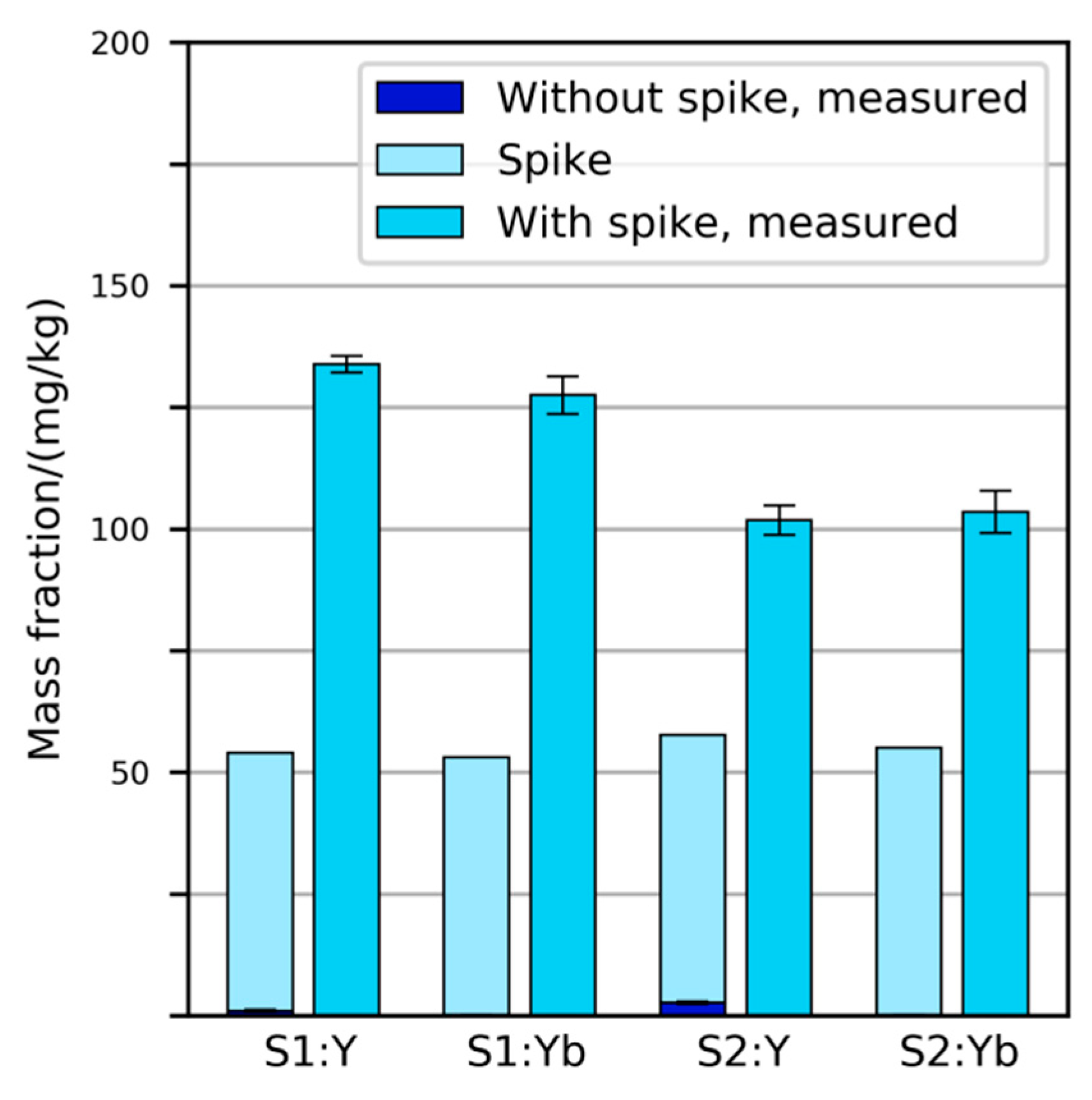
2.2. Spiking of Primary Samples

Before sample preparation, each of the primary samples was spiked with 11.2 g of Y2O3 and 10.0 g of Yb2O3 powders. The amounts added were chosen to result in mass fractions of Y and Yb of around 50 mg/kg, which is much higher than the expected intrinsic content [8]. The spikes were added on the shredder site immediately after collecting the samples. The spikes were sprinkled on top of the samples and manually mixed with the SLF. The spike powders were therefore concentrated in the top layer (approximately the top quarter) of the samples. This was done intentionally to test the ability of the sample preparation process to homogenize the samples.

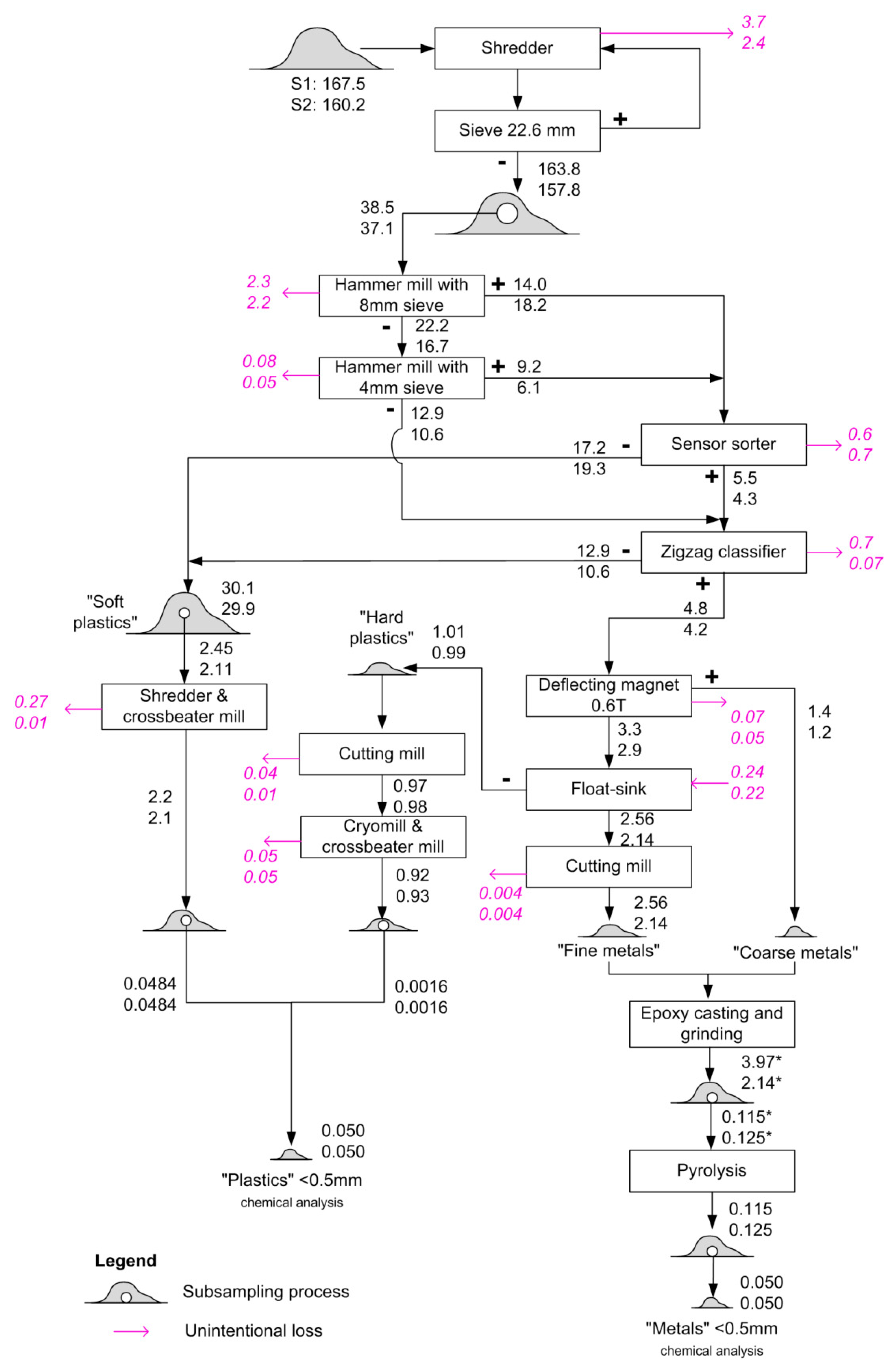
2.3. Physical Sample Preparation

The goal of the sample preparation was to comminute and homogenize the samples of 167.5 kg and 160.2 kg so that representative subsamples of 50 g with a particle size lower than 0.5 mm could be taken for chemical analysis. The main challenge with comminution and homogenization of SLF was the heterogeneity of the material and the presence of different objects with entirely different physical properties, i.e., soft and ductile materials (e.g., plastics, textiles), hard and brittle materials (e.g., glass, ceramics) and hard and ductile materials (metals). A number of single processing lines were first tried out, including briquetting with subsequent cutting, grinding after cooling with liquid nitrogen, pyrolysis, the use of chemical solvents and shredding in various mills. Due to the variable physical properties of the constituents, none of these methods were successful alone in comminuting unsorted SLF. It was therefore decided to use a combination of separation, subsampling and comminution operations: by first separating materials with dissimilar properties (e.g., metals and plastics), comminution operations could be tailored to deal with the characteristic properties of the separate fractions.
The developed procedure is illustrated in Figure 1. The samples were comminuted and homogenized in a shredder until they passed through a sieve with a mesh size of 22.6 mm. After this, they were evenly divided by a ripple divider until a quantity of around 30 kg was reached. The 30 kg was further processed in a hammer mill with a sieve with a mesh size of 8 mm for the first run and a sieve of 4 mm in the second run. The resulting fractions with particle sizes larger than 8 and 4 mm continued to a sensor-sorter for metal separation, where the particles were separated based on electrical conductivity and optical/infrared sensors. The remaining fraction (<4 mm) went directly to a zigzag classifier as the particles were too small to be separated by the sensor-sorter.
The zigzag classifier separated heavy material from light material within a fluidized bed caused by an up-flowing air stream, thereby generating a heavy fraction mainly consisting of metals and harder plastics and a light fraction that mainly consists of soft plastics and textiles. The non-metallic output of the sensor sorter and the light fraction from the zig-zag sorter were combined and are here referred to as the “soft plastics” fraction. This fraction was further divided by a ripple divider to reduce the sample size due to handling capacity (around 3 kg) of the following operations, which involved grinding the sample using a shredding machine followed by a cross beater mill.
The mixture of metals and hard plastics was further processed. A deflecting magnet first separated ferrous metals from the rest, since they are typically very hard and would destroy the cutting mill. In a subsequent float–sink separation, plastics were separated from metals before the resulting fractions were dried for 4–5 h at 110 °C.
The “hard plastics” fraction (an umbrella term for the lighter output of the float–sink separation, mainly consisting of plastics) was further comminuted in a cutting mill, followed by a cryomill and finally, a cross beater mill, to arrive at a particle size of <0.5 mm.
The heavy output from the float–sink separation was further comminuted in a cutting mill, producing a homogenous mixed fine metal fraction. In the next step, this fraction and the previously separated ferrous coarse metals were solidified together in a casting matrix (epoxy), which was then ground in a grinding chamber to reach a particle size of <0.5 mm. Finally, the resulting material was heated to 550 °C to remove the organic epoxy. Part of the metal–epoxy mixture was not heated but retained with the epoxy. This metal–epoxy mixture was used for measuring Cd, which may evaporate during heating to 550 °C.
From the initial ~160 kg of SLF, three final fractions with particle sizes <0.5 mm and a mass of 1–3 kg were produced: “soft plastics”, “hard plastics” and “metals”. Before chemical analysis, the two plastics fractions were mixed together in amounts representing their relative mass shares (97% “soft plastics” and 3% “hard plastics”).

2.4. Chemical Analysis

2.4.1. General Approach

Chemical analysis of the samples was conducted using three different approaches. Firstly, a semi-quantitative analysis of the main metallic elements (Al, Cr, Cu, Fe, Ni, Pb, Sb, Sn and Zn) was performed with wavelength dispersive X-ray fluorescence spectrometry (WD-XRF) at Empa Advanced Analytical Technologies.
Secondly, an element-wise extensive method development was undertaken at Empa Advanced Analytical Technologies to find and validate digestion and measurement methods for each element according to DIN EN ISO/IEC 17025 [36]. This will subsequently be referred to as the “validated method”. These measurement methods were developed based on previous experience with measuring trace metals in SLF and involved, among other things, testing varying acid mixtures, measuring settings and gas reaction modes, as well as the analysis of potentially interfering elements such as oxygen, carbon and halogens. Due to the extensive validation procedure, mass fractions measured using the validated method were expected to be close to the true mass fraction of the digested test samples and are used as reference values in this article.
Thirdly, simplified “in-house” wet-chemical analyses were carried out at Technische Universität Berlin, Chair of Circular Economy and Recycling Technology. These analysis methods are assessed in-house according to national and international guidelines and standards, such as DIN/ISO 11466 [37] and DIN EN ISO/IEC 17025 [36]. These are based on the validated methods but include some simplification to represent typical procedures for routine analyses under normal resource constraints. These simplifications involve using standard measurement settings for general sample matrices and more extensive use of ICP-OES instead of ICP-MS.
The results of the XRF measurements and the in-house method were compared to the results of the validated method to analyse variability and bias of the different methods and to identify particularly difficult cases, i.e., related to specific elements or samples.

2.4.2. Element Selection

A diverse set of 27 elements was chosen for chemical analysis. The elements were selected to include elements that are considered critical to the European Union (Be, Ce, Co, Dy, Ga, Ge, In, La, Mg, Nd, Pd, Pt, Sm) [38], hazardous metals (Cd, Pb, Sb), precious metals (Ag, Au), base metals and some of their common alloying elements (Al, Cr, Cu, Fe, Ni, Sn, Zn), as well as the spiking elements (Y, Yb). The measured elements were expected to occur in the SLF at mass fractions ranging from around 1 mg/kg or less up to several percent. All the elements were measured with the in-house method. Due to the resource requirements of the validated method development, only 19 elements were measured with the validated method. Table 2 lists all the elements measured. In this article, we focus on the 19 elements that were measured with both methods. The observed mass fractions of the remaining elements are included in the Supplementary Materials.

2.4.3. Wavelength Dispersive X-Ray Fluorescence Spectrometry (WD-XRF)

A semi-quantitative analysis was performed with WD-XRF using a Rigaku Primus IV instrument. All samples were prepared for WD-XRF in three different ways: powder samples, wax pellets and fused bead. Powder samples were directly measured with standardless calibration and no additional sample preparation. The detection limit for the elements in the powder samples was approximately 10 mg/kg. For the wax pellets, 2.5 g of Cereox (Wax) was added to 5 g of the sample, and the resulting mixture was pressed with 10 tons (Vaneox-Press). The detection limit for elements in the wax pellets was approximately 50 mg/kg, due to dilution with the wax. For the fusion, 8 g of a mixture of Li2B4O7 and LiBO2 were added to 1 g of the sample in a platinum crucible, and the resulting mixture was melted at 1200 °C in an automatically programmed melting furnace (Fluxana Vitriox). The melt was subsequently transferred into a platinum dish for cooling. The detection limit for the fusion was approximately 200 mg/kg due to dilution with the fluxing agent.

2.4.4. Wet-Chemical Analysis

The same general procedure was followed both for the in-house and the validated method: subsampling of a small portion (0.1–0.2 g) of the physically prepared sample, microwave digestion with HNO3/HCl (aqua regia) or HNO3/H2O2 followed by measurement using inductively coupled plasma optical emission spectrometry (ICP-OES) and/or inductively coupled plasma mass spectrometry (ICP-MS). Detailed information on the wet-chemical analysis methods are provided in Table 3.

2.4.5. Data Analysis

To visually compare the results of the XRF measurements and the in-house measurements with the validated measurements, we calculated the ratio of the mass fraction in each test sample measured with XRF or the in-house method to the mean of the mass fractions measured in the five test samples using the validated method.
An unpaired two-sided t-test was used to detect significant differences between the results of the in-house methods and the validated method. An individual t-test was performed for each combination of sample, element and in-house digestion acid (in total, 152 combinations). A significance level of 0.02 was used to avoid a large number of type I errors. Each t-test compared the 5 values from the validated method with the 3 values from the in-house method. Measurements for which the signal was below the detection limit of the equipment were treated as zeros.

3. Results and Discussion

3.1. Physical Sample Preparation

The two primary samples were spiked with Y2O3 and Yb2O3 powders before physical sample preparation. The amount added corresponded to a mass fraction of 53 mg/kg in sample S1 and 55 mg/kg in sample S2. It was expected that similar mass fractions would be observed by chemical analysis, as the content of these elements in typical SLF from vehicles was believed to be very low (less than 10 mg/kg). After measuring the mass fractions of Y and Yb in the “plastics” and “metals” fractions of the prepared samples and multiplying the result with each fraction’s share in the primary sample, it was found that the prepared samples contained 90–150% more Y and Yb than expected (Figure 2).
By inspecting Figure 3, we see that Y and Yb were preferentially concentrated in the plastics fraction during sample preparation (more than 99% of the spike mass ended up there). Accumulation in the plastics fraction can be explained by the zig-zag sorter, whose purpose is to separate materials with low density (e.g., plastics and textiles) from those with high density (e.g., metals), using an air-stream which carries the light materials up while the heavy materials fall down. In such operations, small but dense particles, such as the spike powders, will also be carried with the light fraction due to their high surface area to mass ratio [39].
The difference between the two elements is small: Y is 5% higher than Yb in sample S1 and 2% lower than Yb in sample S2. This result was expected, as the spikes were added in the same form (fine powder) and the same way (mixed in the top layer of the sample). Hence, their location within the sample volume was correlated from the beginning, and was likely to stay correlated because there is no significant difference in properties that will cause one to behave differently from the other during sample preparation. Any deviation (random or systematic) due to subsampling or losses is therefore likely to have the same sign for the two elements.
There are three possible explanations for the observed difference between the added spike mass fractions and the measured mass fractions: (1) deviations introduced during chemical analysis, (2) intrinsic content of Y and Yb in the primary samples and (3) deviations introduced during physical sample preparation. Significant effects in the validated chemical analysis seem unlikely due to the extensive validation procedures (e.g., as shown in Figure S1, the recoveries from standard addition prior to digestion were 102% and 100% for Y and Yb, respectively). Moreover, problems with digestion are not a plausible explanation since this would lead to underestimation rather than overestimation. Finally, the similarity of the results for the two elements indicates that the observed difference is not due to errors in the chemical analysis.
It also appears very unlikely that the deviation is caused by intrinsic content of the spiking elements in the original samples. Y was independently measured at only 0.9 mg/kg and 2.7 mg/kg in the unspiked samples from the batches of S1 and S2, respectively. These values are in line with findings from a previous study, where Y was measured at 3.5 mg/kg [8]. Yb was measured at around 0.1 mg/kg in the unspiked samples, but was not included in the study by Widmer et al.
Having ruled out these two possible explanations, we conclude that the deviations were mainly introduced during physical sample preparation. To identify possible sources of bias, we inspect the mass losses during sample preparation (shown in magenta in Figure 1). The highest losses were found for the “soft plastics” and “hard plastics” fractions of sample S1 (both 23%). Many of the observed losses were due to oversized particles that were not adequately comminuted and therefore did not pass through the sieves. Considering that the spikes were in powder form, they are unlikely to get lost in this way. Hence, whenever such losses occur, the mass fraction of the spikes would increase, as the total sample mass is reduced but the mass of the spikes in the sample remains the same. Such effects most likely occurred to some extent for both samples, but in particular, for the soft plastics fraction from sample S1 after the crossbeater mill, where 11% of the material was lost. Considering other losses as well, the maximum increase due to losses of non-target constituents would be 30% for sample S1 and 12% for sample S2. This does not explain the whole deviation, but it may explain a large part of the difference between the two samples. The remaining deviation may have occurred during the subsampling steps, and may be due to either systematic or random effects. As the spiking powders were initially concentrated in the top layers of the sample, it is likely that residual heterogeneity led to some deviation from the average concentration during subsampling.
The findings illustrate how the physical properties of particles containing target elements may lead to preferential concentration or dilution during sample preparation and thereby, cause biased results. Whether similar effects influence the results for elements intrinsically contained in SLF is difficult to judge, since it depends on the size and physical properties of the particles in which they are contained, as well as their initial distribution in the primary samples, all of which are largely unknown. However, the spiking trial was an extreme test of the sample preparation procedure given the physical properties of the spikes and their initial heterogeneous distribution in the primary samples. Therefore, the magnitude of the deviation (factor 2) may be considered as an upper boundary of the uncertainty introduced during sample preparation.

3.2. Comparison of Chemical Analysis Methods

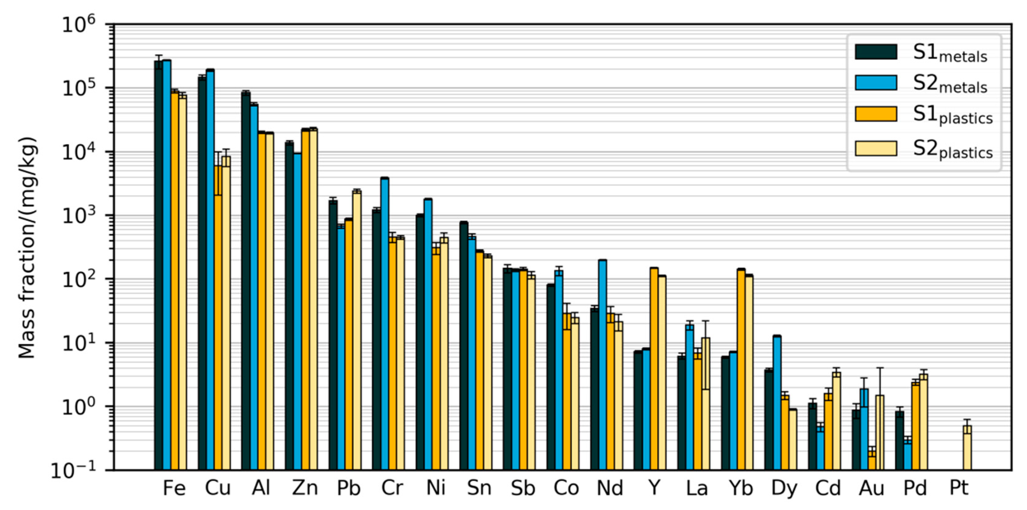
3.2.1. Mass Fractions Measured with Validated Method

Figure 3 displays the absolute mass fractions of 19 elements in the four prepared samples measured using the validated method. Due to the extensive validation of the methods, these will in the following be regarded as the best estimates of the true mass fractions in the prepared samples. The results span a large range of mass fractions, from less than 0.1 mg/kg of Pt in some samples up to 27% Fe in the metals samples. Common metals such as Fe, Al, Cu, Zn were found at above 1% of the mass, while rare earths (Nd, Dy, La) and precious metals (Au, Pd, Pt) were mostly measured at less than 100 mg/kg (0.01%) and less than 10 mg/kg, respectively. Some common alloying elements and other metals such as Cr, Ni, Pb, Sn and Sb were found between 0.01% and 1%. The measured mass fractions are in the same order of magnitude as those from earlier characterizations of ASR. For example, Sn has been measured at 55–350 mg/kg [7,8,32], Nd at 12–130 mg/kg [7,8], and Au up to 1.2 mg/kg [7,8]. However, as the mass fractions found in the present study were measured in sub-fractions of the SLF, they cannot be compared directly to these literature data.
The difference between the two primary samples S1 and S2 is relatively small for the majority of the elements in both of the prepared fractions, indicating consistency in sample preparation and chemical analysis. The observed differences, such as the metal fraction of Nd being higher in S2, may be due to differences between the two batches of cars (S2 is from younger cars than S1) or due to heterogeneity before sub-sampling.
For each element, the measured mass fractions in the plastics and metals fractions are usually quite close (i.e., within the same order of magnitude). This indicates that the sample preparation process is not very efficient at concentrating the elements. For example, Zn was found at higher mass fractions in the plastics fraction than in the metals fraction. The most notable exceptions are Cu, for which the mass fractions are more than 10 times higher in the metals fractions than in the plastics fractions, and the spiking elements Y and Yb, for which the reverse is true.
In the following, we compare the results of the alternative measurement methods (XRF and the in-house methods) to the results of the validated methods and attempt to provide plausible explanations where significant differences occur.

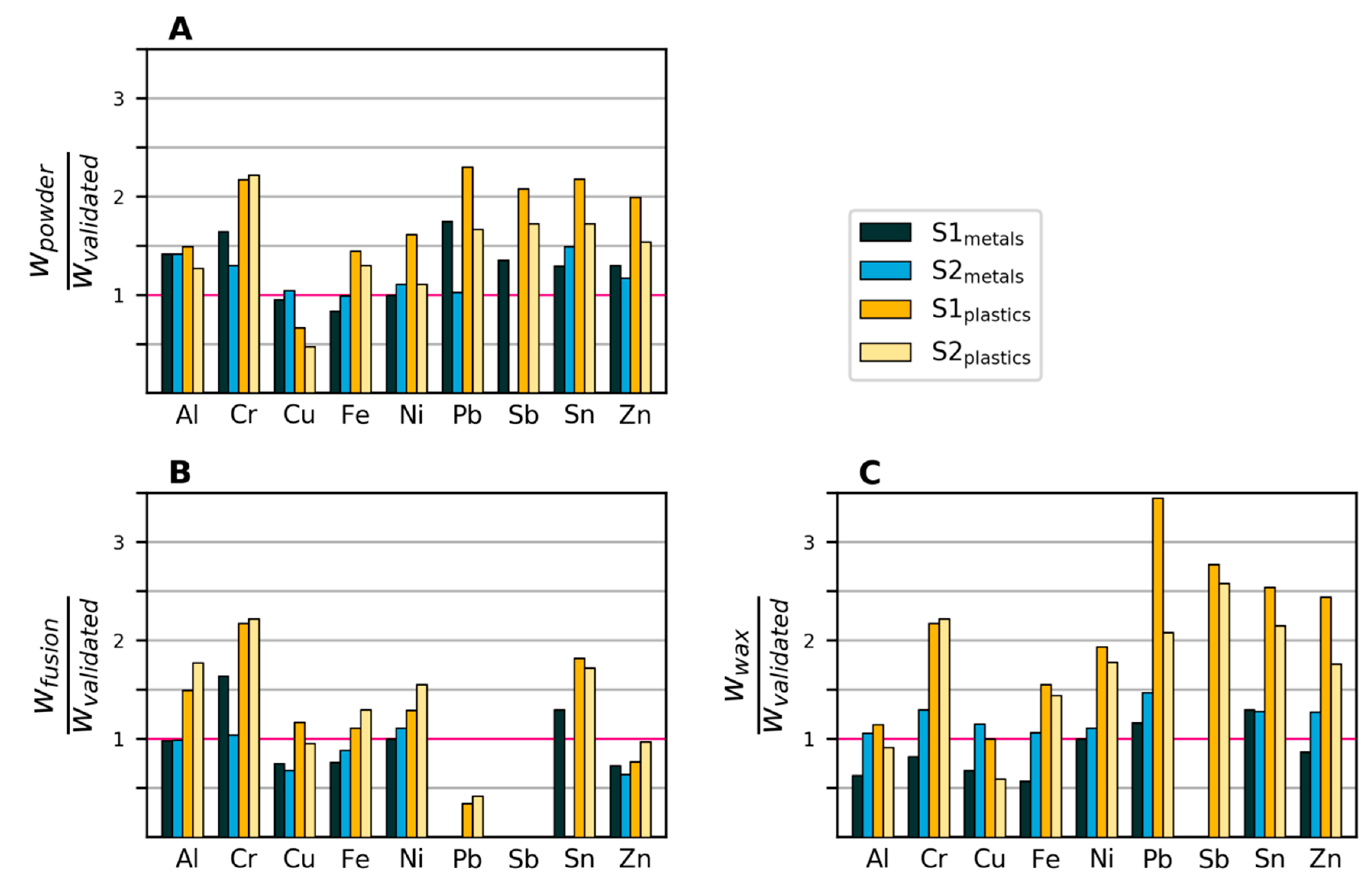
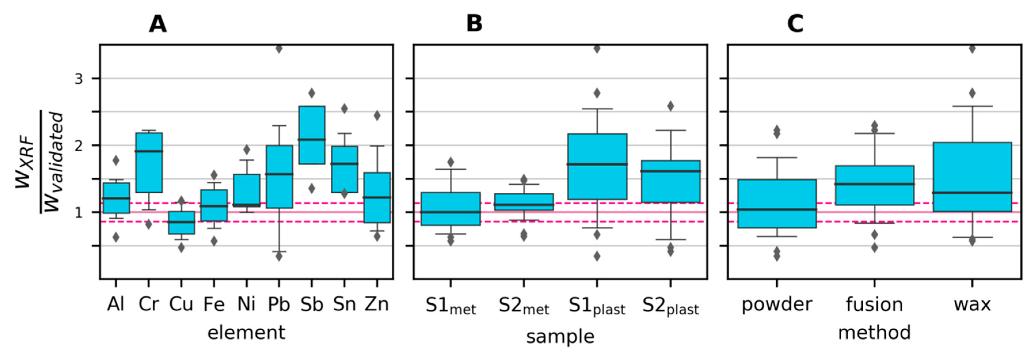
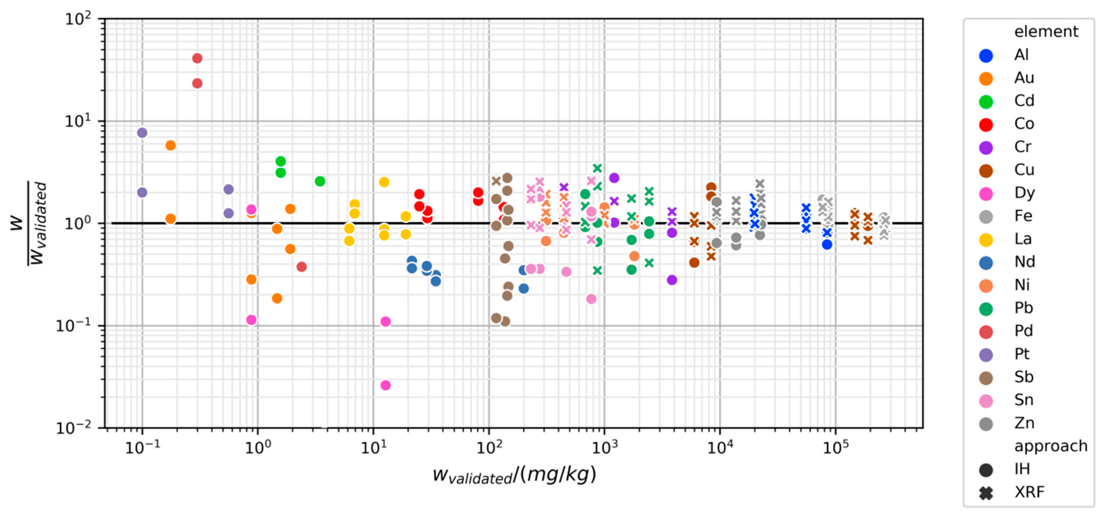
3.2.2. Variability and Bias of XRF Measurements

Figure 4 shows the mass fractions of eight elements in the four samples as measured by XRF, divided by the corresponding mass fractions determined by the validated method. Around half of the measured values lie within +/−50% of those of the validated method. The observed mass fractions from the powder and wax samples were generally higher, on average 40% above the mass fractions measured with the validated method. The results of the XRF fusion method were closer to those of the validated wet chemical analysis (on average, 11% lower). This is expected, as the fusion sample is homogenized and the others are not.
Potential biases and variability in the XRF measurements are visualized in the boxplots in Figure 5, where all observations have been grouped by a) element, b) sample and c) preparation method. For Cr, Sb and Sn, there seems to be a tendency for overestimating the content, especially in the plastics samples. This is likely due to the XRF method being overly sensitive to heavier elements, especially in a light matrix, as is the case for the plastics samples. Figure 5B shows that the plastics samples exhibited both higher variability and lower accuracy compared to the metals samples. Reasons include the plastics samples being more heterogeneous and having element concentrations closer to the detection limit. As seen in Figure 5C, the fusion preparation gave, on average, lower values than the two other preparation methods. This is mainly due to the higher detection limit (caused by dilution), which led to seven cases of non-detection, compared to one case with the direct powder measurement and two cases with wax preparation.

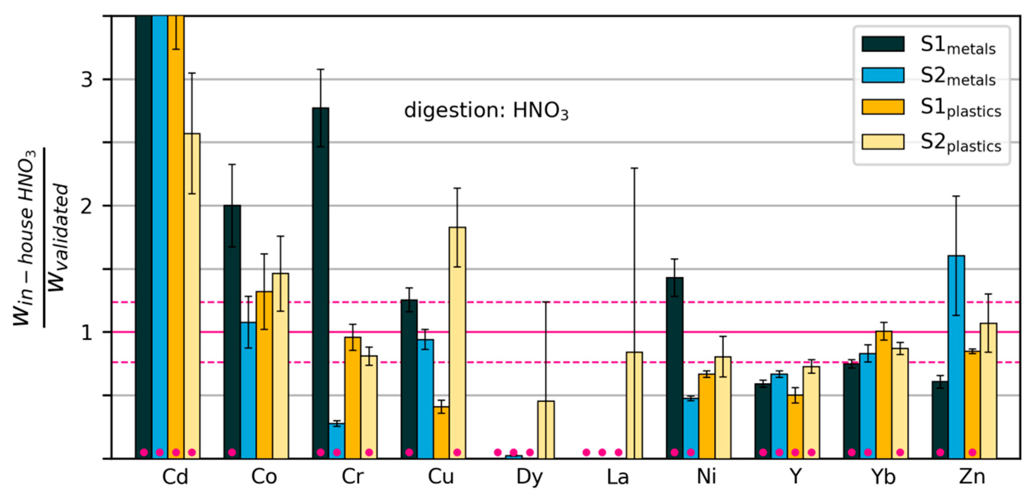
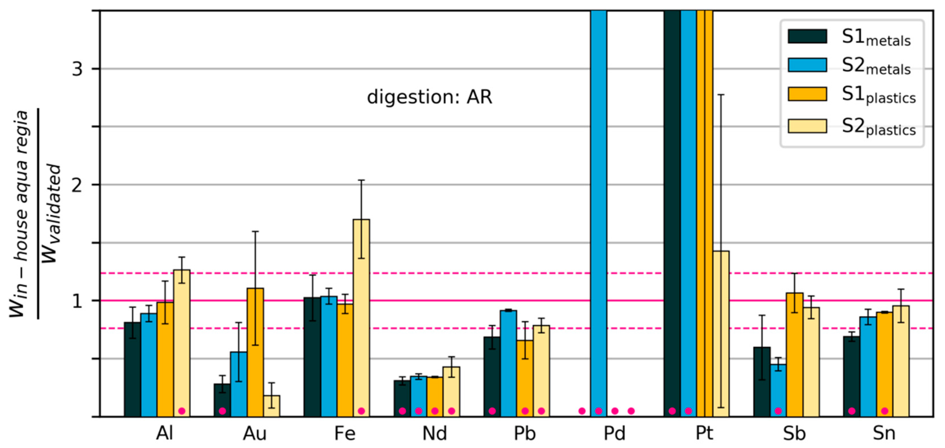
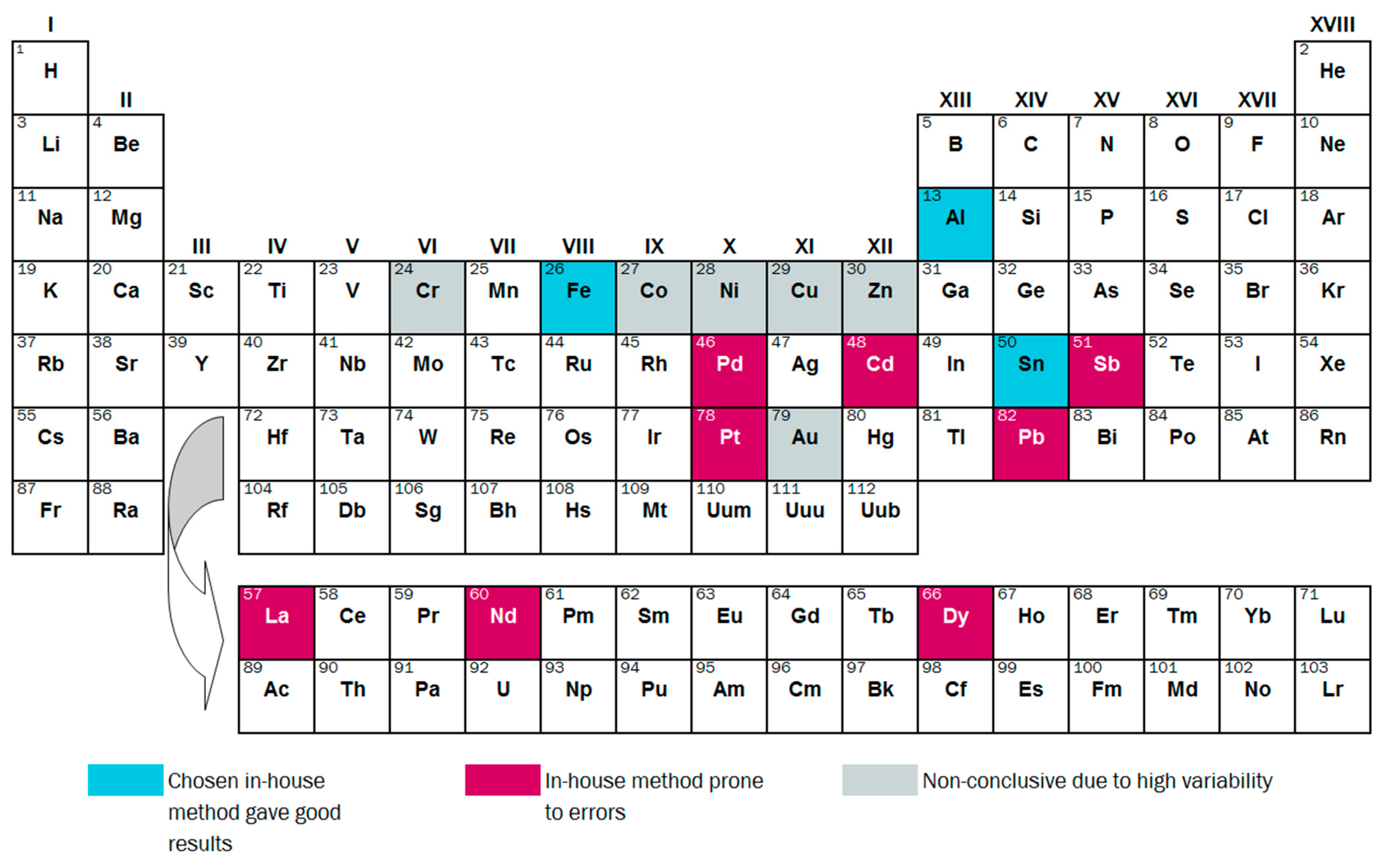
3.2.3. Variability and Bias of In-House Measurements

The results of the in-house wet chemical analysis with HNO3 and aqua regia are shown in Figure 6 and Figure 7, respectively. The measured mass fractions have been normalized by dividing by the corresponding values obtained with the validated method (Figure 3). A two-sided t-test was conducted with the original data for each combination of element, sample and digestion method (in the following referred to as “cases”) to test whether the results obtained by in-house methods were different from those of the validated method. We rejected the null hypothesis of no difference when the p-value of the t-test was lower than 0.02. These cases are marked with pink dots in Figure 6 and Figure 7. All p-values can be found in Table S1.
Inspecting the results of the t-test and the mean deviations between the in-house and validated methods, we can classify the cases into four types: Type 1) the two methods produced results that are significantly different, with a mean relative difference of more than 20%; 2) the two methods gave different results (>20% difference), but the difference is not statistically significant (i.e., they may be due to inhomogeneous samples); 3) the two methods gave similar results (<20% difference), however, there is a small and statistically significant difference; 4) the two methods gave similar results (<20% difference), and there is no significant difference between the results. Type 4 indicates that the in-house method gave similar results as the validated method, while Type 1 and Type 3 indicate that there may be a systematic effect occurring with the in-house method. Type 2 does not allow for any conclusions regarding the suitability of the chemical analysis method.
The results of the classification into deviation types are provided in Table 4. A large number of cases—59% for HNO3 and 44% for aqua regia—are classified as “large significant deviations”, indicating problems with the in-house methods. In only 16% of the cases, in-house digestion with HNO3 gave results similar to the results from the validated method, while with aqua regia, the corresponding number was 33%.
In the following, we will go through the cases by element. We will consider the element well determined by the in-house method when at least three out of four cases (corresponding to the four samples) were classified as Type 3 or Type 4. This condition is fulfilled for Al (aqua regia), Fe (aqua regia), Sn (aqua regia) and the spiking element Yb (HNO3). However, we note that for Yb, there appears to be a small, but systematic underestimation. In addition, Cr, Ni, La and Zn were determined effectively with aqua regia, although this was not the chosen digestion acid with the validated method (see Table S1).
We will consider the method to have clearly failed for a particular element when at least three out of four cases were classified as Type 1 (large significant deviations). This holds true for seven elements: Cd (HNO3), Dy (HNO3), La (HNO3), Nd (aqua regia), Pb (aqua regia), Pd (aqua regia) and the spiking element, Y (HNO3).
Cd was measured at values 2.5–30 times higher with in-house methods than with the validated method in all samples. Dy, La and Pd were clearly underdetermined in three out of four samples with the in-house method. Measurement of these elements with ICP-OES at such low mass fractions (<10 mg/kg) leads to errors, as they are close to the detection limit. For Cd, Dy and Pd, digestion in the other acid system produced similar results, indicating that the problem lies in the detection. The overestimation of Cd may be due to spectral interferences. La was determined effectively using the in-house method with ICP-MS after digestion with AR (see Table S1), indicating that here, detection may also have been the problem. For all four elements, we recommend undertaking measurements with ICP-MS instead. The same applies to Pt, which was clearly overestimated in two out of four samples, and showed very high variability in the remaining two.
Neodymium was measured at mass fractions that were 57% to 69% lower using the in-house method than those obtained using the validated method. The lower values measured with the in-house method indicate a possible problem with digestion, e.g., due to lack of stabilization with additional HCl after digestion. The problem was not detected with standard addition (calculated recovery rates were around 100% and above 140% for metals and plastics samples, respectively). See Figure S1 for details.
In-house measurements of Pb, using aqua regia and ICP-OES, gave results that were 8–34% lower than measurements by the validated method. Possible reasons include incomplete dissolution due to suboptimal digestion parameters (e.g., temperature), interferences with other elements or inadequate calibration of measurement devices.
Y was measured at values 27–50% lower with the in-house method than with the validated method, both methods involve digestion with HNO3 and detection with ICP-MS. A possible explanation is incomplete dissolution of Y2O3. It may be possible to solve the problem by optimising the digestion parameters (time and temperature).
Sb was effectively determined in the plastics samples with the in-house method, but appears to have been underestimated in the metals samples. This could be due to precipitation as Sb2O3. A possible remedy would be to stabilise the aqua regia solution with 2M HCl after digestion. Again, we note that standard addition and calculation of recovery rates did not detect any tendency towards underestimation.
The remaining elements, Au, Co, Cr, Cu, Ni and Zn, were not effectively determined by the chosen in-house method, but also do not show any clear pattern of over- or underestimation. For Au and Cu, it is clear that the samples were not well homogenized. For Cr, Ni and Zn, digestion with aqua regia gave good results (see Table S1). This points towards inconsistencies in the in-house digestion process with HNO3. The suitability of the in-house methods is summarized per element in Figure 8.
Not surprisingly, measuring metal content becomes increasingly challenging at smaller mass fractions. This is illustrated in Figure 9, which displays the mass fractions measured by in-house methods and XRF divided by the mass fractions found with the validated methods on the y-axis and plotted against the mass fractions found with the validated methods on the x-axis. Deviations and bias tend to be higher at smaller mass fractions. Above 100 mg/kg, no elements seem to be severely biased (concentrated on one side of the horizontal black line), and although variability is still high, this may be mostly due to heterogeneity in the samples. Below 100 mg/kg, several measurements seem to be biased. An exception is La, which was relatively well determined with in-house methods despite having a mass fraction of less than 20 mg/kg.

4. Conclusions

SLF is an extremely heterogeneous material that poses a tough challenge to the analyst. The newly developed sample preparation procedure was successful in comminuting all the major constituents of SLF and produced consistent results between the two batches. Despite improvements over existing approaches, some problems were identified through spiking with Y2O3 and Yb2O3 powders. The spiking elements were measured at mass fractions 90–150% higher than expected, pointing towards potential systematic effects during sample preparation. A possible explanation for the observed difference is the preferential concentration of the spike powders due to their small particle size. We therefore propose to conduct spiking of primary samples with materials in different forms, such as metal nuggets, larger metal particles with alloying elements, and plastic particles, as well as fine particles (as was done here). To enable a better comminution of the material and the analysis of larger samples, it should be investigated further whether organic materials can be conveniently removed before sample preparation through a controlled thermal process without loss of target elements.
Three different preparation methods (powder, fused bead, wax pellet) for WD-XRF measurements produced similar results. Preparation of a fused bead led to lower measured mass fractions on average, but this difference can be attributed to a higher detection limit due to dilution. For SLF samples prepared as those described here, with an analyte mass fraction in the range 0.01–10%, WD-XRF delivered results with uncertainties roughly within +100%/−50%. Hence, it can be a good alternative to more expensive wet-chemical analysis when this level of uncertainty is acceptable.
Comparison between results from the in-house chemical analysis and the validated chemical analysis showed that only Al, Fe and Sn were reliably determined with in-house methods. Uncertainties for these elements seem to be roughly +/−20% of the mean. The remaining 16 elements (Au, Cd, Cr, Co, Cu, Dy, La, Nd, Ni, Pb, Pd, Pt, Sb, Y, Yb and Zn) displayed very high variability and/or clearly biased results with in-house methods. In particular, elements below 100 mg/kg require special attention, and are prone to substantial over/under-estimation with routine methods. Most critical are the elements that are close to the detection limit of the instrument (e.g., Cd, Pd and Pt) and/or are not well homogenized (e.g., Au). To improve the reliability and validity of such measurements, we recommend reducing the particle size further (e.g., down to 0.1 mm) before chemical analysis, and possibly using a larger number of repeated digestions.
This study has shown that routine-type analysis of complex materials such as SLF is likely to involve substantial bias and high variability, especially for elements at very low mass fractions (<100 mg/kg). Data on element mass fractions in SLF should therefore be critically examined before being used in other studies, such as material flow analyses or estimations of resource potentials.

Supplementary Materials

The following are available online at https://www.mdpi.com/2313-4321/4/3/34/s1: results of the t-test, recovery rates from standard addition prior to chemical analysis, and plots of all measured mass fractions sorted by element (supplementary pdf document), all measured element mass fractions in individually digested test samples (single_digestions_ppm.csv). All calculated mean values and standard deviations are (mean_sd_ppm.csv). All quantities are given in mg/kg. The datasets are provided in a zip archive Loevik2019_metal_mass_fractions_in_automobile_SLF.zip together with a readme file describing the datasets. The datasets are also available at Zenodo: https://doi.org/10.5281/zenodo.3257054.

Author Contributions

Conceptualization, A.N.L, M.R., R.W., N.K., P.M.M., V.S.R., P.W; formal analysis, A.N.L, R.F., C.S., N.K., P.M.M.; funding acquisition, R.W., V.S.R., P.W.; investigation, A.N.L, R.F., C.S., T.P., C.K., methodology, A.N.L, R.F., C.S., M.R., R.W., R.B., T.P., N.K., C.K., P.M.M., V.S.R., P.W.; project administration, V.S.R., P.W.; supervision, M.R., R.W., R.B., V.S.R., P.W.; validation, A.N.L, R.F., C.S., M.R., N.K., C.K.; visualization, A.N.L, N.K.; writing—original draft, A.N.L; writing—review & editing, A.N.L, R.F., C.S., M.R., R.B., T.P., N.K., P.M.M., V.S.R., P.W.

Funding

This research was funded by the European Union’s Horizon 2020 programme, grant number 641999 (ProSUM project). The shredder batch tests and sampling was funded by the Federal Office for the Environment in Switzerland.

Acknowledgments

The assistance of Melanie Bürki in the experimental part is gratefully acknowledged. Davide Bleiner provided valuable help throughout the project.

Conflicts of Interest

The authors declare no conflicts of interest.

References

  1. Eurostat End-of-life Vehicle Statistics—Statistics Explained. Available online: http://ec.europa.eu/eurostat/statistics-explained/index.php/End-of-life_vehicle_statistics#Total_number_of_end-of-life_vehicles (accessed on 6 March 2018).
  2. Eurostat Treatment of Materials from Shredding within the Member State, by Waste Category, Treatment Type, Country and Year, in Tonnes. Available online: http://ec.europa.eu/eurostat/web/waste/key-waste-streams/elvs (accessed on 9 March 2018).
  3. González-Fernández, O.; Hidalgo, M.; Marguí, E.; Carvalho, M.L.; Queralt, I. Heavy metals’ content of automotive shredder residues (ASR): Evaluation of environmental risk. Environ. Pollut. 2008, 153, 476–482. [Google Scholar] [CrossRef] [PubMed]
  4. Osada, M.; Tanigaki, N.; Takahashi, S.; Sakai, S. Brominated flame retardants and heavy metals in automobile shredder residue (ASR) and their behavior in the melting process. J. Mater. Cycles Waste Manag. 2008, 10, 93–101. [Google Scholar] [CrossRef]
  5. Mancini, G.; Viotti, P.; Luciano, A.; Fino, D. On the ASR and ASR thermal residues characterization of full scale treatment plant. Waste Manag. 2014, 34, 448–457. [Google Scholar] [CrossRef] [PubMed]
  6. The Commission of the European Communities. Commission Decision of 3 May 2000 Replacing Decision 94/3/EC Establishing a List of Wastes Pursuant to Article 1(a) of Council Directive 75/442/EEC on Waste and Council Decision 94/904/EC Establishing a List of Hazardous Waste Pursuant to Article 1(4) of Council Directive 91/689/EEC on Hazardous Waste; The Publications Office of the European Union: Luxembourg, 2000. [Google Scholar]
  7. Ministry of Environment Japan. Report on 2010 Survey to Identify the Characteristics of Automotive Shredder Residue; Ministry of Environment: Tokyo, Japan, 2010. Available online: https://www.env.go.jp/recycle/car/pdfs/h22_report01_mat.pdf (accessed on 30 January 2018).
  8. Widmer, R.; Du, X.; Haag, O.; Restrepo, E.; Wäger, P.A. Scarce Metals in Conventional Passenger Vehicles and End-of-Life Vehicle Shredder Output. Environ. Sci. Technol. 2015, 49, 4591–4599. [Google Scholar] [CrossRef] [PubMed]
  9. Mallampati, S.R.; Lee, C.H.; Truc, N.T.T.; Lee, B.-K. Quantitative analysis of precious metals in automotive shredder residue/combustion residue via EDX fluorescence spectrometry. Int. J. Environ. Anal. Chem. 2015, 95, 1081–1089. [Google Scholar] [CrossRef]
  10. Mallampati, S.R.; Lee, B.H.; Mitoma, Y.; Simion, C. Sustainable recovery of precious metals from end-of-life vehicles shredder residue by a novel hybrid ball-milling and nanoparticles enabled froth flotation process. J. Clean. Prod. 2018, 171, 66–75. [Google Scholar] [CrossRef]
  11. Eurachem, EUROLAB, CITAC, Nordtest and the RSC Analytical Methods Committee. Measurement Uncertainty Arising from Sampling: A Guide to Methods and Approaches, 1st ed.; Ramsey, M.H., Ellison, S.L.R., Eds.; 2007; ISBN 978-0-948926-26-6. Available online: https://eurachem.org/images/stories/Guides/pdf/UfS_2007.pdf (accessed on 31 August 2016).
  12. Gy, P.M. Sampling for Analytical Purposes; John Wiley & Sons Ltd.: Chichester, UK, 1998; ISBN 978-0-471-97956-2. [Google Scholar]
  13. Pineau, J.L.; Kanari, N.; Menad, N. Representativeness of an automobile shredder residue sample for a verification analysis. Waste Manag. 2005, 25, 737–746. [Google Scholar] [CrossRef] [PubMed]
  14. Anzano, M.; Collina, E.; Piccinelli, E.; Lasagni, M. Lab-scale pyrolysis of the Automotive Shredder Residue light fraction and characterization of tar and solid products. Waste Manag. 2017, 64, 263–271. [Google Scholar] [CrossRef] [PubMed]
  15. Khodier, A.; Williams, K.; Dallison, N. Challenges around automotive shredder residue production and disposal. Waste Manag. 2017, 73, 566–573. [Google Scholar] [CrossRef] [PubMed]
  16. Haydary, J.; Susa, D.; Gelinger, V.; Čacho, F. Pyrolysis of automobile shredder residue in a laboratory scale screw type reactor. J. Environ. Chem. Eng. 2016, 4, 965–972. [Google Scholar] [CrossRef]
  17. Totland, M.; Jarvis, I.; Jarvis, K.E. An assessment of dissolution techniques for the analysis of geological samples by plasma spectrometry. Chem. Geol. 1992, 95, 35–62. [Google Scholar] [CrossRef]
  18. Joint Committee for Guides in Metrology GUM: Guide to the Expression of Uncertainty in Measurement. Available online: http://www.bipm.org/en/publications/guides/gum.html (accessed on 17 February 2016).
  19. Gy, P.M. Sampling of discrete materials—A new introduction to the theory of sampling: I. Qualitative approach. Chemom. Intell. Lab. Syst. 2004, 74, 7–24. [Google Scholar] [CrossRef]
  20. Agenzia Nazionale per la Protezione dell’Ambiente (ANPA). La Caratterizzazione del Fluff di Frantumazione Dei Veicoli; Agenzia Nazionale per la Protezione dell’Ambiente (ANPA): Rome, Italy, 2002; ISBN 88-448-0057-8. [Google Scholar]
  21. Agenzia per la protezione dell’ambiente e per i servizi tecnici (APAT). Studio APAT/ARPA Sul Fluff di Frantumazione Degli Autoveicoli; Agenzia per la Protezione Dell’ambiente e per i Servizi Tecnici (APAT): Rome, Italy, 2006; ISBN 88-448-0181-7. [Google Scholar]
  22. Ahmed, N.; Wenzel, H.; Hansen, J.B. Characterization of Shredder Residues generated and deposited in Denmark. Waste Manag. 2014, 34, 1279–1288. [Google Scholar] [CrossRef] [PubMed]
  23. Börjeson, L.; Löfvenius, G.; Hjelt, M.; Johansson, S.; Marklund, S. Characterization of automotive shredder residues from two shredding facilities with different refining processes in Sweden. Waste Manag. Res. 2000, 18, 358–366. [Google Scholar] [CrossRef]
  24. Day, M.; Shen, Z.; Cooney, J.D. Pyrolysis of auto shredder residue: Experiments with a laboratory screw kiln reactor. J. Anal. Appl. Pyrolysis 1999, 51, 181–200. [Google Scholar] [CrossRef]
  25. Galvagno, S.; Fortuna, F.; Cornacchia, G.; Casu, S.; Coppola, T.; Sharma, V.K. Pyrolysis process for treatment of automobile shredder residue: Preliminary experimental results. Energy Convers. Manag. 2001, 42, 573–586. [Google Scholar] [CrossRef]
  26. Mancini, G.; Tamma, R.; Viotti, P. Thermal process of fluff: Preliminary tests on a full-scale treatment plant. Waste Manag. 2010, 30, 1670–1682. [Google Scholar] [CrossRef] [PubMed]
  27. Mayyas, M.; Pahlevani, F.; Handoko, W.; Sahajwalla, V. Preliminary investigation on the thermal conversion of automotive shredder residue into value-added products: Graphitic carbon and nano-ceramics. Waste Manag. 2016, 50, 173–183. [Google Scholar] [CrossRef] [PubMed]
  28. Mirabile, D.; Pistelli, M.I.; Marchesini, M.; Falciani, R.; Chiappelli, L. Thermal valorisation of automobile shredder residue: Injection in blast furnace. Waste Manag. 2002, 22, 841–851. [Google Scholar] [CrossRef]
  29. Morselli, L.; Santini, A.; Passarini, F.; Vassura, I. Automotive shredder residue (ASR) characterization for a valuable management. Waste Manag. 2010, 30, 2228–2234. [Google Scholar] [CrossRef]
  30. Notarnicola, M.; Cornacchia, G.; De Gisi, S.; Di Canio, F.; Freda, C.; Garzone, P.; Martino, M.; Valerio, V.; Villone, A. Pyrolysis of automotive shredder residue in a bench scale rotary kiln. Waste Manag. 2017, 65, 92–103. [Google Scholar] [CrossRef] [PubMed]
  31. Roy, C.; Chaala, A. Vacuum pyrolysis of automobile shredder residues. Resour. Conserv. Recycl. 2001, 32, 27. [Google Scholar] [CrossRef]
  32. Santini, A.; Morselli, L.; Passarini, F.; Vassura, I.; Di Carlo, S.; Bonino, F. End-of-Life Vehicles management: Italian material and energy recovery efficiency. Waste Manag. 2011, 31, 489–494. [Google Scholar] [CrossRef] [PubMed]
  33. Zolezzi, M.; Nicolella, C.; Ferrara, S.; Iacobucci, C.; Rovatti, M. Conventional and fast pyrolysis of automobile shredder residues (ASR). Waste Manag. 2004, 24, 691–699. [Google Scholar] [CrossRef] [PubMed]
  34. Lyn, J.A.; Ramsey, M.H.; Fussell, R.J.; Wood, R. Measurement uncertainty from physical sample preparation: Estimation including systematic error. Analyst 2003, 128, 1391–1398. [Google Scholar] [CrossRef] [PubMed]
  35. Korf, N.; Løvik, A.N.; Figi, R.; Schreiner, C.; Kuntz, C.; Mählitz, P.M.; Rösslein, M.; Wäger, P.; Rotter, V.S. Multi-element chemical analysis of printed circuit boards—Challenges and pitfalls. Waste Manag. 2019, 92, 124–136. [Google Scholar] [CrossRef] [PubMed]
  36. International Organization for Standardization (ISO). ISO/IEC 17025:2005: General Requirements for the Competence of Testing and Calibration Laboratories; International Organization for Standardization: Geneva, Switzerland, 2005. [Google Scholar]
  37. International Organization for Standardization (ISO). ISO 11466: Soil Quality—Extraction of Trace Elements Soluble in Aqua Regia; International Organization for Standardization: Geneva, Switzerland, 1995. [Google Scholar]
  38. European Commission. Study on the Review of the List of Critical Raw Materials; European Commission: Brussels, Belgium, 2017. [Google Scholar]
  39. Bunge, R. Mechanische Aufbereitung: Primär—und Sekundärrohstoffe; 1. Auflage.; Wiley-VCH Verlag GmbH & Co. KGaA: Weinheim, Germany, 2012; ISBN 978-3-527-33209-0. [Google Scholar]
Figure 1. Mechanical sample preparation process for SLF. The numbers refer to the related mass flows in kg from sample S1 (top) and S2 (bottom). Magenta arrows indicate unintentional losses, determined by weighing the inputs and outputs of each operation. The numbers marked with an asterisk (*) refer to the “metals” content excluding the added epoxy.
Recycling 04 00034 g001
Figure 2. Mass fractions of Y and Yb expected and measured in spiked SLF samples S1 and S2. In all four instances, the measured values were substantially higher than expected. Error bars indicate standard deviation of five repeated digestions/measurements.
Recycling 04 00034 g002
Figure 3. Mass fractions of elements measured with the validated method. Error bars show standard deviations from digestion and measurement of five test samples of 0.2 g each. Note that Y and Yb have been added to the primary samples.
Recycling 04 00034 g003
Figure 4. Mass fractions (w) measured with XRF divided by mass fractions measured with the validated method. Values that are zero indicate that the element was not detected. A: XRF powder. B: XRF fused bead. C: XRF wax pellet.
Recycling 04 00034 g004
Figure 5. Mass fractions (w) measured by XRF divided by mass fractions measured by the validated method. The median is shown as a thick blue line, boxes represent the 25th to 75th percentile, whiskers represent the 5th and 95th percentile, and outliers are shown as circles. The horizontal pink dashed lines show the relative standard deviation of the validated measurements across all elements. (A): grouped by element; (B): grouped by sample; (C): grouped by XRF sample preparation method.
Recycling 04 00034 g005
Figure 6. Mass fractions measured by “in-house” digestion in HNO3/H2O2, relative to mass fractions measured with the validated method. The dashed horizontal lines show the relative standard deviation of the validated measurements across all elements. Error bars extend one standard deviation above and below the mean (calculated from three repeated digestions/measurements). Pink dots indicate that the measurements were significantly different from those of the validated method (p < 0.02). Some values are too large to be displayed within the limits of the y-axis (see Table S1).
Recycling 04 00034 g006
Figure 7. Mass fractions measured by “in-house” digestion in aqua regia, relative to mass fractions measured with the validated method. The dashed horizontal lines show the relative standard deviation of the validated measurements across all elements. Error bars extend one standard deviation above and below the mean (calculated from three repeated digestions/measurements). Pink dots indicate that the measurements were significantly different from those of the validated method (p < 0.02). Some values are too large to be displayed within the limits of the y-axis (see Table S1).
Recycling 04 00034 g007
Figure 8. Overview of conclusions regarding the suitability of in-house methods for measuring 17 elements in SLF.
Recycling 04 00034 g008
Figure 9. Mass fractions measured by in-house methods and XRF divided by corresponding mass fractions measured by validated methods (y-axis) versus mass fractions measured by validated methods (x-axis). Distance from the horizontal black line represents the deviation from validated result. Larger deviations are seen at low mass fractions.
Recycling 04 00034 g009
Table 1. Description of primary shredder light fraction (SLF) samples taken after shredding end-of-life vehicles (ELVs).
SampleVehicle Cohort YearsMass/kg
S11988–2000167.5
S22001–2015160.2
Table 2. Elements measured.
Element GroupElements Measured
Base metalsAl, Cu, Fe, Zn
Precious metalsAg *, Au, Pd, Pt
Rare earth elementsCe *, Dy, La, Nd, Sm *, Y, Yb
Other elementsBe *, Cd, Co, Cr, Ga *, Ge *, In *, Mg *, Ni, Pb, Sb, Sn
* Elements measured only with the in-house method.
Table 3. Wet-chemical analysis procedures.
In-House MethodValidated Method
Microwave digestion
Device nameCEM MarsXpressMLS START
Acid 1): mixture6 mL HNO3 69% (Roth suprapur) + 1 mL H2O2 35% (Merck pro analysi)6 mL HNO3 67–69% (VWR Chemicals Normatom)+ 1 mL H2O2 30% (Merck suprapur)
Acid 1): elements measuredAl, Ag, Au, Be, Cd, Ce, Co, Cr, Cu, Dy, Fe, Ga, Ge, In, La, Mg, Nd, Ni, Pb, Pd, Pt, Sb, Sm, Sn, Y, Yb, Zn (all)Cd, Co, Cr, Cu, Dy, La, Ni, Y, Yb, Zn
Acid 2): mixture5.25 mL HCl 35% (Roth suprapur) + 1.75 mL HNO3 (Roth suprapur)5.25 mL HCl 30% (Merck suprapur) +1.75 mL HNO3 67–69% (VWR Chemicals Normatom)
Acid 2): elements measuredAl, Ag, Au, Be, Cd, Ce, Co, Cr, Cu, Dy, Fe, Ga, Ge, In, La, Mg, Nd, Ni, Pb, Pd, Pt, Sb, Sm, Sn, Y, Yb, Zn (all)Al, Au, Fe, Nd, Pb, Pd, Pt, Sb, Sn
Digestion programmeStepHold time/minPower/WTemp/°CStepHold time/minPower/WTemp/°C
16160015016700150
25160020025800200
3181600215318800215
4251600045800240
Sample mass digestedapproximately 0.1 g0.2 g
Number of digestionsn = 3n = 5
Final volume and dilution50 mL, filled up with 0.5 mol/L HNO3 for acid mixtures 1) and 2)50 mL, filled up with H2O. for 1) and with 2 mol/L HCl for 2)
Validationelement spikes added before digestionelement spikes added before digestion; certified standard reference material
Analytical determination
ICP-OES device nameThermo Scientific iCap 6000 Series Varian Vista Pro Radial
ICP-OES elementsAl, Ag, Au, Be, Cd, Ce, Co, Cr, Cu, Dy, Fe, Ga, Ge, In, La, Mg, Nd, Ni, Pb, Pd, Pt, Sb, Sm, Sn, Y, Yb, Zn (all elements)Al, Cr, Cu, Fe, Ni, Pb and Zn
ICP-MS device nameThermo Scientific iCap QAgilent 8800 QQQ
ICP-MS collision modeHeHe
ICP-MS elementsAu, Ce, In, La, YAu, Cd, Co, Dy, Nd, La, Pd, Pt, Sb, Sn, Y, Yb
Table 4. Number of cases with significant differences (p < 0.02) between in-house and validated methods.
|δ| > 20%|δ| < 20%
SignificantInsignificantSignificantInsignificant
HNO324 (55%)5 (11%)5 (11%)6 (14%)
aqua regia16 (44%)5 (14%)3 (8%)12 (33%)

